




No CrossRef data available.
Article contents
RUIN PROBABILITY UNDER COMPOUND POISSON MODELS WITH RANDOM DISCOUNT FACTOR
Published online by Cambridge University Press: 22 January 2004
Abstract
In this article, we consider a compound Poisson insurance risk model with a random discount factor. This model is also known as the compound filtered Poisson model. By using some stochastic analysis techniques, a convergence result for the discounted surplus process, an expression for the ruin probability, and the upper bounds for the ruin probability are obtained.
Information
- Type
- Research Article
- Information
- Probability in the Engineering and Informational Sciences , Volume 18 , Issue 1 , January 2004 , pp. 55 - 70
- Copyright
- © 2004 Cambridge University Press
1. INTRODUCTION
Recently, the interplay between actuarial science and finance has attracted much attention. One important question is, “What happens if we consider the investment risk in the insurance risk model?” There are many recent articles in actuarial science literature which tackle this problem. Sundt and Teugels [13] considered a compound Poisson model with a constant interest rate. Renewal-type equations satisfied by the ruin probability, asymptotic expression, and the upper bounds for the ruin probability were obtained. Yang and Zhang [15] extended the work in Sundt and Teugels [13] and considered the joint distribution of the surplus immediately before and after ruin. Yang [14] considered a discrete model with a constant interest rate. By using martingale inequalities, both exponential and nonexponential bounds were obtained. Paulsen [10] and Norberg [9] used diffusion models with stochastic interest incomes. Paulsen and Gjessing [11] provided some results for a model with stochastic investment incomes. Asmussen [2] summarized some recent works on ruin probability with investment income.
Delbaen and Haezendonck [5] considered the risk theory problems in an economic environment by discounting the value of the surplus from the current (or future) time to the initial time. The present article is in the spirit of Delbaen and Haezendonck [5], but whereas they used a deterministic discount factor, we will use a random discount factor. This is somewhat the same as when we consider the compound Poisson model with a stochastic interest rate. We call the model a filtered compound Poisson model.
This article is organized as follows. Section 2 provides the model and assumptions, Section 3 obtains a convergence result for the discounted surplus process, Section 4 gives an expression for the ruin probability, Section 5 discusses the constant interest force and exponential claim case, Section 6 obtains some upper bounds for the ruin probability, and the last section deals with the case of negative security loading.
2. THE MODEL
The classical risk model can be described as follows:

where U(t) denotes the surplus at time t, u denotes the initial surplus, c denotes the premium rate in a unit time, Xi denotes the amount of the ith claim, and N(t) denotes the number of claims occurring in the time interval (0, t] . It is assumed that {N(t); t > 0} is a homogeneous Poisson process with an intensity of λ. It is also assumed that the claim amounts are independent of the claim number process and are positive and mutually independent and identically distributed (i.i.d.) with common distribution function F, where F satisfies F(0) = 0. Moreover, we assume that F has a mean p1 and

We assume that

where θ is called security loading. We assume that θ > 0 in the first part (up to Section 6) of this article, and we discuss the case where θ ≤ 0 in Section 7.
In the literature, there are many articles dealing with the ruin problems for the classical risk model. However, in the real world, investment income plays a very important role. In this article, we consider the insurance risk model where the interest rate is random. Let Ti denote the ith claim time and let Wt denote the discount factor. The discounted value of total claim amounts occurring in the time interval (0, t] can then be described as

S = {St} is called a filtered Poisson process. Using the properties of the filtered Poisson process (see Deng and Liang [6] or Snyder [12]), we have


where σ(Ws : 0 ≤ s < t) denotes the σ-field generated by {Ws : 0 ≤ s < t}.
Assuming that the interest rate is random (equivalently, the discount factor Wt is random), similar to (2.1), the surplus process of an insurance company can then be described by the following model:

where Ut(W) denotes the discounted value of the surplus (discounted from time t to time 0) and all the other notations remain the same as earlier. We call model (2.5) the compound filtered Poisson model.
In this article, we make the following assumptions:
1. {Wt}, {Xi}, and {N(t)} are mutually independent.
2. W0 = 1, and Wt > 0 for all t > 0, a.e.
The first assumption is a common one in actuarial science. Although, recently, there have been some works on the dependent risk in the actuarial literature, we do not consider this issue here. The second assumption states that the interest rate cannot be positive infinity. Our model here is very general. In practice, we usually assume that the interest rate is nonnegative at any time. This corresponds to Wt > 0 and Wt is nonincreasing for all t > 0.
3. CONVERGENCE OF Ut(W)
In this section, we will prove a convergence result. This convergence result will then be used in later sections to prove some useful results in the insurance risk theory. In this section, we assume that the discount factor Wt satisfies the following assumption:

Under the above assumption, we have the following result.
Theorem 1: Under assumption (3.1), there exists an integrable random variable U∞(W) such that

and

where a.e. means almost everywhere with respect to probability measure P. Moreover, the characteristic function of U∞W is given by

Proof: Let

Then, Mt is a martingale with a mean of zero, and Mt is independent of the discount factor Wt. Using this notation, the discounted surplus can be rewritten as

where

is also a martingale with a mean of zero.
First, we will prove the convergence of

. Since Ws is nonnegative for all s ≥ 0, the monotone convergence theorem implies

because

The random variable

is P − a.s. finite, which proves the convergence of

. Next, we will prove the convergence of Ht. Note that {Ht} is an L2-bounded martingale; the result follows from a standard result. Therefore, there exists a finite random variable H∞ such that

From the above results, we see that there exists a finite random variable U∞(W) such that

The characteristic function of U∞W is obtained by straightforward calculation. █
Remark 1: It is well known that for the classical compound Poisson model, if θ > 0, the surplus process will move toward +∞ with a probability 1 as the time t → ∞. This means that in the classical compound Poisson model, if we let the surplus process continue even when the ruin occurs, the surplus process will eventually become very large (tend to infinity with probability 1 as time tends to infinity). See Dassios and Embrechts [4], for further detailed discussions on this issue. Theorem 1 tells us that if we include the interest effect in the model, this is not the case.
4. AN EXPRESSION OF RUIN PROBABILITY
Ruin probability has been one of the most important research topics for almost a century, ever since the pioneering work of Lundberg [7,8]. Elegant mathematics has been developed on this topic.
In this section, we will use the result of Theorem 1 to give an expression for the ruin probability. Let T(u) = inf{t; Ut(W) < 0} and ψ(u) denote the ruin probability of model (2.5). Then,

Let

; then,

Let

then,

Notice that Ut has stationary and independent increments and that it is independent of Wt. If we assume

then we can obtain that

where

Remark 2: Because we do not require that Wt be nonincreasing in this article, any Levy processes will satisfy assumption (*).
Lemma 1: The process {Ut(W)}, condition on σ(Ws : 0 ≤ s < t), has an independent increment, and under assumption (*),

where

means that both the left-hand side and the right-hand side of (4.4) have the same distribution.
Proof: For t > s > 0,

Notice that {Wt} is independent of {N(t) : t ≥ 0} and {Xi : i = 1,2,…}, so

has independent increments and is independent of Ws. Therefore, this lemma holds. █
From the above results, we have the following theorem.
Theorem 2: Under assumption (*), let F∞(x) be the distribution function of U∞(W) − u. Then,

Proof:

Here, we have used the notation

. From this, the result is proved. █
We say that a distribution function F(x) is a new worse than used (NWU) distribution if F(x) is a distribution function (d.f.) of a nonnegative random variable and ÝF(x) = 1 − F(x) satisfies that ÝF(x)ÝF(y) ≤ ÝF(x + y) for x ≥ 0 and y ≥ 0. We say that a distribution function F(x) is a new better than used (NBU) distribution if F(x) is a d.f. of a nonnegative random variable and satisfies that ÝF(x)ÝF(y) ≥ ÝF(x + y) for x ≥ 0 and y ≥ 0.
Proposition 1: Under assumptions (3.1) and (*), we have the following:
1. If Xi's distribution function is NWU, then, in this case, we have that

2. If Xi's distribution function is NBU, then, in this case, we have
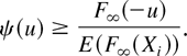
3. If Xi's distribution function is exponential, then, in this case, we have

Proof: We only give the proof for part 1 because part 2 can be proved by the same method, and part 3 can be obtained from parts 1 and 2 because the exponential distribution is both NWU and NBU.

where T(u)− means the time just before ruin.
When U∞(W) − u > 0, we can get from the distribution of Xi is NBU, that the above probability is less than P{Xi > U∞(w) − u}—that is, the value E(F∞(Xi)). When U∞(w) − u < 0, the above probability is 1 and the value P{Xi > U∞(w) − u} also equals one.
After all, when the distribution of Xi is NBU, we have

so we can get part 1. █
Remark 3:
1. When F∞(0) > 0, we have

2. From the expression

we can say that F∞(−u) is just the probability of ruin for good (i.e., the probability of the surplus tends to negative infinity).
3. It is interesting that the ruin probability can be determined by the limit distribution of the discounted surplus process. Theorem 2 indicates the relationship between the ruin probability and the limit distribution of the discounted surplus process.
5. CONSTANT DISCOUNT RATE AND EXPONENTIAL CLAIM SIZE
We consider a special case in which the discount rate is a constant δ and the claim size is an exponentially distributed random variable. This case was treated in Sundt and Teugels [13]. We will obtain this result as a special case of our results in the previous sections. In this section, we will assume that Wt = e−δt and Xi is exponentially distributed with a mean of p1. We will first give Lemma 2.
Lemma 2: The discounted value of all of the claim amounts occurring in the time interval (0, t],

, converges to a random variable S(+∞). Furthermore, S(+∞) has a gamma distribution with parameters (λ/δ, p1−1).
Proof: According to the properties of the filtered Poisson process, we can derive the characteristic function of S(t) by (see Snyder [12])

Let t → +∞; then,

The characteristic function of S(+∞) is then

This is the characteristic function of a gamma-distributed random variable with parameters (λ/δ, p1−1). Therefore, the lemma holds. █
As explained in Remark 4, part 2 that follows, the following theorem gives the same result as that in Sundt and Teugels [13].
Theorem 3: Under the assumptions in this section, the ruin probability ψ(u) of model (2.5) has the following expression:

where FΓ(λδ−1, p1−1)(·) denotes the distribution function of the Γ random variable with the parameters (λδ−1, p1−1).
Proof: Under the assumptions in this section, model (2.5) becomes

From Lemma 2, we know that

where S(+∞) is gamma-distributed with the parameters (λ/δ, p1−1), (i.e., u + [(1 + θ)/δ] p1λ − Ut(W) converges to a Γ random variable with the parameters (λ/δ, p1−1)). Then, using Theorem 2, the result is proved. █
Remark 4:
1. Notice that
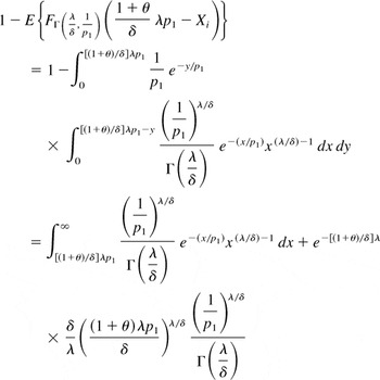
Therefore, the result in Theorem 3 is the same as that in Sundt and Teugels [13].
2. The result in Theorem 3 was obtained in Sundt and Teugels [13] by solving the associated renewal equation. We have obtained the result here by using the limit distribution of the surplus process. Therefore, we have, in fact, provided more information than in Sundt and Teugels [13]; that is, we have also proved that the limit distribution of the discounted surplus process is a gamma distribution.
6. UPPER BOUNDS FOR RUIN PROBABILITY
In this section, we will derive the upper bounds for ruin probability. The main results are given in the following two theorems. The techniques used in the proof are similar to those in Yang [14].
Theorem 4: Suppose that G(·) is a nonnegative measurable function, Ut(W) is the discounted surplus of the insurance company at time t, and G(Ut(W)) is a supermartingale with respect to σ-field

. Then,

If limt→∞ E(G(Ut(W))|T(u) > t) = 0 and G(Ut(W)) is an

martingale, then

where T(u) is the same as earlier.
Proof: T(u) is an

stopping time. For ∀t > 0, T(u) ∧ t is a bound

stopping time. Using Doob's bounded stopping time theorem, we have

Let t → +∞; by the positive of G(·), we have

Therefore, (6.1) holds.
Moreover, if limt→+∞ E(G(UT(u)(W))|T(u) > t) = 0 and G(Ut(W)) is an

martingale, then (6.2) also holds. █
Theorem 5: If, for all t ≥ 0, 0 < Wt < 1 a.e., assume that there exists R > 0 such that

Then,

Proof: For all x ∈ (0,1] , y > 0,

holds; that is,

Let h(r) = E(erXi − 1). Because for all t > 0, 0 < Wt < 1 a.e, we then have

Let

Using a similar argument as that in Deng and Liang [6, pp.329–332] (also see Snyder [12]) and after some calculations, we obtain

so

Therefore, Nt is an

supermartingale. From Theorem 4, we have

where R > 0 and UT(u)(W) < 0. Note that E [exp(−RUT(u)(W))|T(u) < ∞] > 1. Therefore, the result of the theorem holds. █
7. UPPER BOUNDS FOR RUIN PROBABILITY IN THE CASE OF NEGATIVE LOADING
It is well known that, in the classical model, if the loading is negative, the ruin becomes certain. We will show below that this is not the case in the model with stochastic interest rate. We first introduce the following sets:


From the definition, we can easily see that D is an interval of the form (0, r) or (0, r] . It is not difficult to see that for 0 < t < ∞, we have Dt = D if D = (0, r] , and if D = (0, r) with r < ∞, then Dt = (0, r) or (0, r] . Furthermore, if 0 < t and u < ∞, then Dt = Du.
It is not difficult to prove that the assumption

implies that D∞ = Dt.
The following theorem provides us with an upper bound for ruin probability in the case of negative safety loading.
Theorem 6: Assume that the safety loading θ ≤ 0 and 0 < t < ∞. Then, we have the following results:


Proof: For r ∈ Dt, let h(r) = E [exp(rX1)] − 1 and define

With the same arguments as in the proof of Theorem 5, it is not difficult to check that Mt is a martingale with respect to

, where

Applying Doob's bounded stopping time theorem to the martingale {Mt : t ∈ R+} for the stopping time T ∧ t, 0 < t < ∞, we have

where I{A} denotes the indicator function of set A, and we have used the fact that, at the ruin time T,

.
Hence, if r ≥ 0,

Therefore,

From the inequality ex − 1 ≥ x, θ ≤ 0, and that Ws and X1 are positive random variables, we have that

Hence, (7.6) can be rewritten as

From this, the theorem follows. █
Notice that the upper bounds in theorem 6 only make sense if the right-hand sides of (7.6) and (7.7) are smaller than one. We will address this problem now.
For 0 < t ≤ ∞, let


Proposition 2: Suppose that 0 < t ≤ ∞ and the safety loading θ ≤ 0. Φt(r) is then a convex mapping on R+ and is finite on Dt.
Proof: Similar to Lemma 4.5 of Delbaen and Haezendonck [5], we can prove the following:
If

then

If

then

From this, it follows that Φt(r) is a convex mapping on R+. It is obvious that Φt(r) is finite on Dt.
The above analysis indicates that infr≥0 Φt(r) < 1 if the right derivative of Φt(r) at r = 0 is strictly negative. However,

where the last equality holds because X1 and Ws are independent. This leads to the following proposition.
Proposition 3: If 0 < t < ∞ and

there exists a real number rt > 0 such that

Furthermore, if

there exists a real number r∞ > 0, such that

We conclude this section by giving two special cases. First, we consider the classical compound Poisson model (Ws = 1). In this case, if the risk loading θ is negative, the ultimate ruin probability will be one. The upper bound for the ruin probability at a finite time, say before time t, is nontrivial if

The second case is the situation with a constant interest force. In this case, Ws = e−δs. A detailed discussion on this case can be found in Boogaert and Crijins [3].
Acknowledgments
The authors would like to thank Professor Elias Shiu for pointing out an error and some problems with the model in the earlier version of this article. This work was supported by grants from Research Grants Council of HKSAR (project no. HKU 7139/01H) and the Natural Science Foundation of China (grant 19831020).
References
REFERENCES
Aczel, J. &
Dhombres, J.
(1989).
Functional equations in several variables: With applications to
mathematics, information theory and to the natural and social
sciences.
New York:
Cambridge University Press.CrossRef
Asmussen, S.
(2000).
Ruin probabilities.
Singapore:
World Scientific.
Boogaert, P. &
Crijins, V.
(1987).
Upper bounds on ruin probabilities in case of negative loadings and
positive interest rate.
Insurance: Mathematics and Economics
6:
221–232.Google Scholar
Dassios, A. &
Embrechts, P.
(1989).
Martingales and insurance risk.
Communications in Statistics—Stochastic Models
5:
181–217.Google Scholar
Delbaen, F. &
Haezendonck, J.
(1987).
Classical risk theory in an economic environment.
Insurance: Mathematics and Economics
6:
85–116.Google Scholar
Deng, Y.L. &
Liang, Z.S.
(1992).
Stochastic point processes and applications.
Beijing:
Science Publisher
(in Chinese).
Lundberg, F.
(1903).
I. Approximerad Framstallning af Sannolikhetsfunktionen. II.
Aterforsakring af Kollektivrisker.
Uppsala:
Almqvist and Wiksells.
Lundberg, F.
(1926).
Forsakringsteknisk Riskutjamning.
Stockholm:
F. Englunds Boktryckeri.
Norberg, R.
(1999).
Ruin problems with asset and liabilities of diffusion type.
Stochastic Processes and Their Applications
81:
255–269.Google Scholar
Paulsen, J.
(1998).
Ruin theory with compounding assets—A survey.
Insurance: Mathematics and Economics
22:
3–16.Google Scholar
Paulsen, J. &
Gjessing, H.K.
(1997).
Ruin theory with stochastic return on investments.
Advances in Applied Probability
29:
965–985.Google Scholar
Snyder, D.L.
(1975).
Random point processes.
New York:
Wiley.
Sundt, B. &
Teugels, J.L.
(1995).
Ruin estimates under interest force.
Insurance: Mathematics and Economics
16:
7–22.Google Scholar
Yang, H.
(1999).
Non-exponential bounds for ruin probability with interest effect
included.
Scandinavian Actuarial Journal
1999:
66–79.Google Scholar
Yang, H. &
Zhang, L.
(2001).
The joint distribution of surplus immediately before ruin and the
deficit at ruin under interest force.
North American Actuarial Journal
5(3):
92–103.Google Scholar
 You have
Access
- 6
- Cited by