1. Introduction
The prediction of the concentration distribution of scalar mixtures in porous media is a key element for the quantification of mixing and reactive transport processes (e.g. Dentz et al. Reference Dentz, Le Borgne, Englert and Bijeljic2011), and the assessment of uncertainty and risk for contaminant transport in the subsurface (e.g. Tartakovsky Reference Tartakovsky2013). The development of predictive models for these purposes requires upscaling the impact of flow heterogeneity on effective transport. To this end, one would ideally wish to rely on solid guidelines to describe the entire concentration field in a given medium, for given injection conditions. In the context of porous media, the discussion has historically been mostly confined to a particular aspect of the overall problem, namely the dispersive properties of the medium. By ‘dispersive’, we mean the description of the extent of the spatial spreading of the mixture, or of its residence time in the vicinity of a given point in the medium (see e.g. Danckwerts Reference Danckwerts1953; Bear Reference Bear1972; De Gennes Reference De Gennes1983; Gelhar & Axness Reference Gelhar and Axness1983; Dagan Reference Dagan1987; Bouchaud & Georges Reference Bouchaud and Georges1988; Koch et al. Reference Koch, Cox, Brenner and Brady1989; Cushman, Hu & Ginn Reference Cushman, Hu and Ginn1994; Attinger et al. Reference Attinger, Dentz, Kinzelbach and Kinzelbach1999; Dentz et al. Reference Dentz, Kinzelbach, Attinger and Kinzelbach2000; Delgado Reference Delgado2007). Field measurements and laboratory experiments have thus prompted research to understand the scale dependence of global dispersion coefficients and its relation to the medium heterogeneity, the influence of the possible presence of traps and dead zones for the transported substances, as well as the validity of the advection–dispersion equation in describing large-scale solute transport (e.g. Berkowitz et al. Reference Berkowitz, Cortis, Dentz and Scher2006; Neuman & Tartakovsky Reference Neuman and Tartakovsky2009). However, the spatial extent of a mixture does not tell us much about its content but rather its average concentration, and knowledge of the spreading properties alone is insufficient to quantify mixing (e.g. Kitanidis Reference Kitanidis1994; Dentz et al. Reference Dentz, Le Borgne, Englert and Bijeljic2011; Le Borgne et al. Reference Le Borgne, Dentz, Davy, Bolster, Carrera, de Dreuzy and Bour2011), that is, the full concentration distribution, and the local spatial structure of the concentration field in the medium.
Mixing processes in porous media are particularly important for controlling fluid–fluid as well as fluid–solid chemical reactions (e.g. Cirpka & Valocchi Reference Cirpka and Valocchi2007; Cirpka et al. Reference Cirpka, Schwede, Luo and Dentz2008; Rolle et al. Reference Rolle, Eberhardt, Chiogna, Cirpka and Grathwohl2009; Dentz et al. Reference Dentz, Le Borgne, Englert and Bijeljic2011; de Anna et al. Reference de Anna, Jimenez-Martinez, Tabuteau, Turuban, Le Borgne, Derrien and Méheust2014b ). Dissolution or precipitation processes, for instance, are often triggered by the mixing of different waters respectively at chemical equilibrium (e.g. Tartakovsky et al. Reference Tartakovsky, Redden, Lichtner, Scheibe and Meakin2008). Different mixing measures have been studied to investigate these processes in porous media (Kitanidis Reference Kitanidis1994; Fiori & Dagan Reference Fiori and Dagan2000; Fiori Reference Fiori2001; Le Borgne et al. Reference Le Borgne, Dentz, Bolster, Carrera, de Dreuzy and Davy2010; Chiogna et al. Reference Chiogna, Hochstetler, Bellin, Kitanidis and Rolle2012; De Barros et al. Reference De Barros, Dentz, Koch and Nowak2012; Bolster et al. Reference Bolster, Valdes-Parada, Le Borgne, Dentz and Carrera2011). The dynamics of mixing can be fully quantified by the temporal evolution of the concentration probability density function (PDF), as the mixture evolves towards uniformity under the combined action of diffusion and advection. A common approach used is to assume an ad hoc distribution, which is parametrized from analytical derivation of concentration moments obtained under different approximations (e.g. Fiorotto & Caroni Reference Fiorotto and Caroni2002; Bellin & Tonina Reference Bellin and Tonina2007; Cirpka et al. Reference Cirpka, Schwede, Luo and Dentz2008; Tonina & Bellin Reference Tonina and Bellin2008). Other approaches include mapping closures to transfer the stochasticity of the flow field to the concentration distribution (e.g. Chen, Chen & Kraichnan Reference Chen, Chen and Kraichnan1989; Dentz & Tartakovsky Reference Dentz and Tartakovsky2010; Dentz Reference Dentz2012) and phenomenological approaches employing stochastic mixing models (Valiño & Dopazo Reference Valiño and Dopazo1991; Fedotov, Ihme & Pitsch Reference Fedotov, Ihme and Pitsch2005) to simulate the stochastic evolution of concentration using surrogate mechanisms; see also Pope (Reference Pope2000) and Fox (Reference Fox2004) for an overview.
The study of scalar mixing in a simple stirring protocol by Meunier & Villermaux (Reference Meunier and Villermaux2010) has nevertheless demonstrated that these mechanisms can be quantified from first principles using the powerful concept of the ‘diffusive strip’, or ‘lamellae’ representation of the scalar field (Ranz Reference Ranz1979). Scalar lamellae are naturally formed by the repeated action of advective motions. In this representation the coupling of diffusion to the stretching experienced by the lamellae is straightforward. The complete PDF of concentration can thus be computed from the diffusion equation in a moving frame, and an additional principle of lamellae random coalescence initially proposed by Villermaux & Duplat (Reference Villermaux and Duplat2003) allows for the description of the mixture content up to its final uniformity. In the same vein, we have recently highlighted the role of stretching, diffusion and coalescence mechanisms in governing the evolution of concentration mixtures in Darcy scale porous media (Villermaux Reference Villermaux2012; Le Borgne, Dentz & Villermaux Reference Le Borgne, Dentz and Villermaux2013). While the porous media structure does not deform in general, the ‘frozen’ flow heterogeneity at different scales generates folding and stretching mechanisms similar to those in chaotic or turbulent flows (Metcalfe et al. Reference Metcalfe, Lester, Ord, Kulkarni, Trefry, Hobbs, Regenaur-Lieb and Morris2010; De Barros et al. Reference De Barros, Dentz, Koch and Nowak2012; Mays & Neupauer Reference Mays and Neupauer2012; Villermaux Reference Villermaux2012). In this framework, the understanding of the basic composition rule of the dispersing mixture provides an analytical description of the overall concentration distribution.
We explore here the potential of this theory for predicting mixing in Darcy scale heterogeneous porous media over a range of Péclet numbers and structural heterogeneities. The main challenge when dealing with these highly heterogeneous flow systems is that dispersion and mixing occur simultaneously. This leads to a range of mixing behaviours, at the extremes of which lie two turbulent flow equivalents: the ever-dispersing mixture scenario (Duplat, Innocenti & Villermaux Reference Duplat, Innocenti and Villermaux2010) for large Péclet numbers, and the confined mixture scenario (Duplat & Villermaux Reference Duplat and Villermaux2008) for small Péclet numbers. In the first case, the concentration content can be determined from the stretching history of individual lamellae alone, while for the second case, the concentration content is given by the frequency of coalescence of neighbouring lamellae. The large flow heterogeneity induced by the underlying permeability structures implies the existence of an extended intermediate regime, characterized by partial lamellae coalescence and the persistence of concentration lacunarities in the mixture. This regime is also characterized by pre-asymptotic super-diffusive dispersion, which is known to persist over a large range of temporal and spatial scales in heterogeneous porous media (e.g. Berkowitz et al. Reference Berkowitz, Cortis, Dentz and Scher2006; Neuman & Tartakovsky Reference Neuman and Tartakovsky2009). As discussed in this study, super-diffusive spreading has a direct impact on the stretching behaviour and on the evolution of concentrations within the scalar mixture.
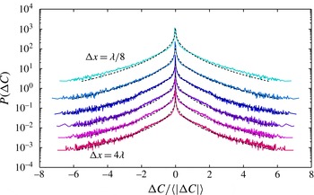
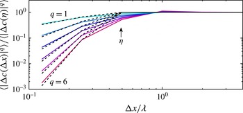
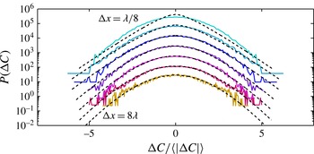
We investigate these processes in the light of a lamellar mixing model using numerical simulations of the full Darcy scale flow and transport problem, which allows for the detailed measurement of the lamellae deformation and concentration contents of the mixture. By tagging a line of passive scalar perpendicular to the mean flow in a well-characterized heterogeneous permeability field, we analyse in §§ 2–5 the Lagrangian stretching distribution and correlations in detail, and in §§ 6 and 7 the evolution of concentration PDFs in relation to the geometry of material lines and their coalescence frequency. Furthermore, we discuss the impact of the medium heterogeneity on the mixing behaviour, as quantified by different mixing measures in §§ 8 and 9, as well as on the spatial structure of the concentration fields through the analysis of the PDF of concentration increments in § 10.
2. Flow and transport in heterogeneous permeability fields
In this section we introduce the basic flow and transport equations and their boundary and initial conditions, as well as their numerical solution. We consider two-dimensional heterogeneous conductivity fields, where the conductivity
 $K(\boldsymbol{x})$
is represented as a lognormally distributed random field. The joint distribution of the point values of log-conductivity
 $f(\boldsymbol{x})=\ln K(\boldsymbol{x})$
is multivariate Gaussian and characterized by a mean
 $\overline{f}$
variance
 ${\it\sigma}_{f}^{2}$
and correlation length
 ${\it\lambda}$
. The correlation function of the fluctuations of
 $f(\boldsymbol{x})$
is taken as Gaussian
 $C_{f}(\boldsymbol{x})=\exp [-\boldsymbol{x}^{2}/(2{\it\lambda}^{2})]$
. This type of random conductivity is generic as it allows representation of a range of spatial variability and correlation properties observed in natural permeability fields (e.g. Gelhar Reference Gelhar1993). As such, it represents a reference field for theories of flow and transport in heterogeneous porous media (e.g. Fiori & Dagan Reference Fiori and Dagan1999; Cirpka & Valocchi Reference Cirpka and Valocchi2007; Le Borgne, Dentz & Carrera Reference Le Borgne, Dentz and Carrera2008). Since porosity is known to vary over a much narrower range than permeability (e.g. Bear Reference Bear1972; Gelhar Reference Gelhar1993), the impact of porosity heterogeneity on solute transport is generally considered subdominant compared to spatial variability in hydraulic conductivity. Thus we consider here a constant porosity in order to restrain the space of parameters to be explored. The methodology may, however, be extended to consider porosity variations as well.
Spatial variability of the conductivity
 $K(\boldsymbol{x})$
is mapped onto the divergence-free flow field
 $\boldsymbol{u}(\boldsymbol{x})$
via the Darcy equation
 $\boldsymbol{u}(\boldsymbol{x})=-K(\boldsymbol{x})\boldsymbol{{\rm\nabla}}h(\boldsymbol{x})$
, with
 $h(\boldsymbol{x})$
the hydraulic head. We assume that fluid and porous media are both incompressible so that continuity is expressed by
 $\boldsymbol{{\rm\nabla}}\boldsymbol{\cdot }\boldsymbol{u}(\boldsymbol{x})=0$
. The flow is driven by a uniform in the mean head gradient due to constant head boundary conditions at the lateral domain boundaries. At the horizontal boundaries no-flow conditions are applied. The mean head gradient and the geometric mean conductivity are set to one so that the average flow velocity is unity. Note that all spatial dimensions are normalized to the conductivity correlation length and all temporal scales to the advection time so that results may be applicable to corresponding field cases upon appropriate rescaling.
We consider here non-reactive transport through the divergence-free Darcy flow field
 $\boldsymbol{u}(\boldsymbol{x})$
described above. The transport of concentration
 $c(\boldsymbol{x},t)$
is described by the Fokker–Planck equation
 $$\begin{eqnarray}\frac{\partial c(\boldsymbol{x},t)}{\partial t}+\boldsymbol{u}(\boldsymbol{x})\boldsymbol{\cdot }\boldsymbol{{\rm\nabla}}c(\boldsymbol{x},t)-D{\rm\nabla}^{2}c(\boldsymbol{x},t)=0.\end{eqnarray}$$
In general, dispersion is a tensorial quantity and depends on the Darcy velocity
 $\boldsymbol{u}(\boldsymbol{x})$
. For the sake of simplicity, and to focus on the impact of advective heterogeneity, local dispersion is modelled by a constant dispersion coefficient
 $D$
. Time is rescaled with constant porosity
 ${\it\phi}$
such that
 $t=t^{\prime }/{\it\phi}$
, where
 $t^{\prime }$
is the simulation time. As boundary conditions for concentration, we impose
 $\boldsymbol{n}_{v}\boldsymbol{\cdot }D\boldsymbol{{\rm\nabla}}c(\boldsymbol{x},t)=0$
at the vertical boundaries, and zero normal flux, that is,
 $\boldsymbol{n}_{h}\boldsymbol{\cdot }[\boldsymbol{u}(\boldsymbol{x})-D\boldsymbol{{\rm\nabla}}]c(\boldsymbol{x},t)=0$
at the horizontal boundaries, where
 $\boldsymbol{n}_{v}$
and
 $\boldsymbol{n}_{h}$
are the outward-pointing unit normal vectors at the vertical and horizontal boundaries respectively. The initial condition is given by an instantaneous uniform line injection at
 $x_{1}={\it\lambda}$
such that
 $c(\boldsymbol{x},0)=L^{-1}{\it\delta}(x_{1}-{\it\lambda})$
, where
 $L$
is the extension of the domain perpendicular to the mean flow direction. Notice that we choose an initial plume that integrates a representative part of the heterogeneity spectrum in order to systematically quantify the impact of stochastic flow fluctuations on the mixing behaviour. In the opposite case of point-like solute injection, the initial mixing behaviour is expected to be different (De Barros et al.
Reference De Barros, Dentz, Koch and Nowak2012).
The characteristic advection time scale is defined by
 ${\it\tau}_{a}={\it\lambda}/\overline{u}$
, where
 $\overline{u}$
is the mean transport velocity. The characteristic diffusion time is
 ${\it\tau}_{D}={\it\lambda}^{2}/D$
. The Péclet number
 $$\begin{eqnarray}Pe=\frac{{\it\lambda}\overline{u}}{D}\end{eqnarray}$$
compares the diffusive and advective time scales.
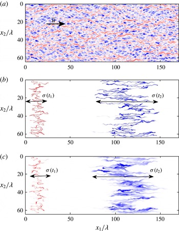
(a) Computed velocity field for a realization of a permeability field with
 ${\it\sigma}_{f}^{2}=1$
. Corresponding concentration fields
 $c(\boldsymbol{x},t)$
for (b)
 $\mathit{Pe}=8\times 10^{4}$
and (c)
 $\mathit{Pe}=8\times 10^{2}$
at times
 $t_{1}=12.5{\it\tau}_{a}$
(red) and
 $t_{2}=112.5{\it\tau}_{a}$
(blue), for an initial injection with a uniform concentration
 $c_{0}$
at
 $x_{1}={\it\lambda}$
. The plume is transported from left to right with a mean velocity
 $\overline{u}$
and a dispersion length
 ${\it\sigma}(t)$
increasing with time.

The transport equation (2.1) is solved by random walk particle tracking using
 $N_{p}=10^{7}$
particles based on the equivalent Langevin equation
 $$\begin{eqnarray}\frac{\text{d}\boldsymbol{x}(t|\boldsymbol{a})}{\text{d}t}=\boldsymbol{u}[\boldsymbol{x}(t|\boldsymbol{a})]+\sqrt{2D}{\bf\xi}(t),\end{eqnarray}$$
where
 ${\bf\xi}(t)$
is a Gaussian white noise of zero mean and unit variance, and
 $a$
is the initial tracer injection location,
 $\boldsymbol{x}(t=0|\boldsymbol{a})=\boldsymbol{a}$
. The flow equation
 ${\rm\Delta}h(\boldsymbol{x})+\boldsymbol{{\rm\nabla}}f(\boldsymbol{x})\boldsymbol{\cdot }\boldsymbol{{\rm\nabla}}h(\boldsymbol{x})=0$
is solved numerically with a finite difference scheme. The flow domain is the two-dimensional rectangle
 ${\it\Omega}=\{\boldsymbol{x}|x_{1}\in [0,819.2{\it\lambda}],x_{2}\in [0,102.4{\it\lambda}]\}$
. Both flow and transport are solved numerically using the numerical modelling platform H2OLAB (http://h2olab.inria.fr).
The PDF
 $p_{c}(c,t)$
of concentration point values is obtained by spatially sampling all concentration values in the domain that are above a concentration threshold
 ${\it\epsilon}$
. This defines the characteristic volume
 $V_{c}(t)$
that is occupied by the solute
 $$\begin{eqnarray}V_{c}(t)=\int _{c(\boldsymbol{x},t)>{\it\epsilon}}\text{d}\boldsymbol{x}.\end{eqnarray}$$
Figure 1(a) displays an example of the simulated velocity field for a moderately heterogeneous permeability field, with
 ${\it\sigma}_{\ln K}^{2}=1$
. The corresponding concentration fields at
 $t_{1}=12.5{\it\tau}_{a}$
and
 $t_{2}=112.5{\it\tau}_{a}$
are shown in figure 1(b,c), for an initial injection with a uniform concentration
 $c_{0}$
at longitudinal position
 $x_{0}={\it\lambda}$
, for different Péclet numbers. The scalar line, initially located perpendicular to the main flow direction, distorts into a brush with a typical streamwise width
 ${\it\sigma}$
, increasing in time. The brush is made of a collection of strips, aligned on average with the direction of the mean flow. Similar behaviours can be observed for solute plumes originating from different extended initial distributions. The deformation action of the flow field on the fluid support eventually leads to the creation of laminar structures such as the ones observed here for a uniform initial concentration along a line.
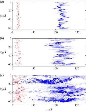
For large Péclet numbers, the scalar concentration is close to uniform along the stretching direction, and varies rapidly along the compressive direction, thus forming a lamella-like topology (Ottino Reference Ottino1989). Hence, the concentration field can be seen as a set of lamellae, whose concentration depends on the interaction between local stretching and diffusion. Compression perpendicular to the stretching direction enhances diffusive smoothing by steepening the scalar gradient. For small Péclet numbers, neighbouring lamellae overlap by diffusive coalescence. The concentration field is then composed of lamella aggregates and concentration lacunarities in areas with small lamella density. The permeability field heterogeneity has a strong impact on the concentration distribution as it determines the distribution of stretching rates along the mixing front and the frequency of lamella coalescence: see figure 2. In the following, we formalize the roles of these different processes in building up the overall concentration distribution.
Concentration fields
 $c(\boldsymbol{x},t)$
at times
 $t_{1}=12.5{\it\tau}_{a}$
(red) and
 $t_{2}=112.5{\it\tau}_{a}$
(blue) for
 $\mathit{Pe}=8\times 10^{2}$
and for different permeability field variances: (a)
 ${\it\sigma}_{f}^{2}=0.25$
, (b)
 ${\it\sigma}_{f}^{2}=1$
and (c)
 ${\it\sigma}_{f}^{2}=4$
.

3. Local interaction between stretching and diffusion
We recall here the basic interaction between stretching and diffusion at the scale of a lamella, leading to an expression for the concentration PDF across a strip that depends on the stretching history (Ranz Reference Ranz1979; Duplat et al.
Reference Duplat, Innocenti and Villermaux2010; Meunier & Villermaux Reference Meunier and Villermaux2010). Considering a single lamella, the temporal evolution of the concentration
 $c({\it\zeta},t)$
at a position
 ${\it\zeta}$
along the direction perpendicular to the lamella is
 $$\begin{eqnarray}\frac{\partial c}{\partial t}+\frac{{\it\zeta}}{s}\frac{\text{d}s}{\text{d}t}\frac{\partial c}{\partial {\it\zeta}}=D\frac{\partial ^{2}c}{\partial {\it\zeta}^{2}},\end{eqnarray}$$
where
 $D$
is the diffusion coefficient and
 $s(t)$
is the distance between two material particles in the direction perpendicular to the lamella. By mass conservation under pure advection,
 $s(t)$
is related to the lamella length
 $\ell (t)$
by
 $s(t)\ell (t)=s_{0}\ell _{0}$
, where
 $s_{0}$
and
 $\ell _{0}$
are the initial lamella dimensions. Therefore
 $s^{-1}\text{d}s/\text{d}t=-\ell ^{-1}\text{d}\ell /\text{d}t$
. For the initial condition
 $c({\it\zeta},t=0)=c_{0}\exp (-{\it\zeta}^{2})$
, the solution is given by the Gaussian profile,
 $$\begin{eqnarray}c({\it\zeta},t)=\frac{c_{0}\exp \!\left[-\displaystyle \frac{{\it\zeta}^{2}{\it\rho}(t)^{2}}{s_{0}^{2}(1+4{\it\tau}(t))}\right]}{\sqrt{1+4{\it\tau}(t)}},\end{eqnarray}$$
where we have defined the dimensionless time
 $$\begin{eqnarray}{\it\tau}(t)=\frac{D}{s_{0}^{2}}\int _{0}^{t}\text{d}t^{\prime }{\it\rho}(t^{\prime })^{2}\end{eqnarray}$$
from the relative strip elongation
 ${\it\rho}(t)=\ell (t)/\ell _{0}$
. The maximum lamella concentration
 ${\it\theta}$
in
 ${\it\zeta}=0$
is
 $$\begin{eqnarray}{\it\theta}(t)=\frac{c_{0}}{\sqrt{1+4{\it\tau}(t)}}.\end{eqnarray}$$
The concentration PDF in the strip corresponding to the Gaussian profile (3.2) is given by
 $$\begin{eqnarray}p(c|{\it\theta})=\frac{1}{2c\sqrt{\ln ({\it\theta}/{\it\epsilon})\ln ({\it\theta}/c)}}\end{eqnarray}$$
with
 ${\it\theta}\geqslant c$
. The concentration range is
 $[{\it\epsilon},{\it\theta}]$
, with
 ${\it\epsilon}$
and
 ${\it\theta}$
the minimum and maximum concentrations in the strip. Equation (3.5) provides the relationship between the concentration PDF of a lamella and its elongation history, through the temporal evolution of the maximum concentration (3.4) in the strip.
4. Statistics of Lagrangian elongations
In this section we analyse the stretching of lamellae in the heterogeneous flow field using the explicit numerical simulations. The stretching process is then represented by a multiplicative stochastic process that models the series of Lagrangian deformation events, and thus the stretching history.
The history of relative lamella elongation
 ${\it\rho}(t)$
can be quantified by computing the pair separation
 $\ell (t)=|\boldsymbol{x}(t|\boldsymbol{a}+{\rm\Delta}\boldsymbol{a})-\boldsymbol{x}(t|\boldsymbol{a})|$
of neighbouring particles initially located at a distance
 $\ell _{0}=|{\rm\Delta}\boldsymbol{a}|$
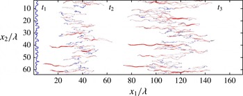
on the injection line. Figure 3 displays the location of
 $5\times 10^{5}$
advective particles at different times, initially separated by a distance
 $\ell _{0}=1.25\times 10^{-4}{\it\lambda}$
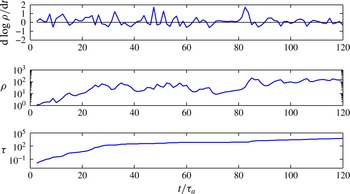
. An example of Lagrangian elongation history for a particle pair is given in figure 4. The stretching rate
 ${\it\gamma}(t)$
in the following is defined by
 $$\begin{eqnarray}{\it\gamma}(t)=\frac{1}{{\it\rho}(t)}\frac{\text{d}{\it\rho}(t)}{\text{d}t}.\end{eqnarray}$$
Strong stretching events are typically followed by compression events, with a small effect on the net elongation (figure 4). Significant variations of the elongation occur during localized events characterized by a succession of positive elongation rates. In between these events, the total elongation rate remains approximately constant. The dimensionless time
 ${\it\tau}(t)$
, which controls the maximum lamella concentration (3.3), also changes significantly during the positive stretching events. In between these events, it evolves linearly with time as the elongation is approximately constant.
Advected line at times
 $t_{1}=2.5{\it\tau}_{a}$
,
 $t_{2}=37.5{\it\tau}_{a}$
,
 $t_{3}=112.5{\it\tau}_{a}$
for
 ${\it\sigma}_{f}^{2}=1$
. The initial position of the line is
 $x_{1}={\it\lambda}$
. The red colour intensity is proportional to
 ${\it\rho}$
for lamella elongations
 ${\it\rho}\geqslant 10$
. The blue colour intensity is proportional to
 $1/{\it\rho}$
for
 ${\it\rho}<10$
. Hence, the red zones represent the parts of the line that are most elongated while the blue zones represent the portions that have been less stretched.

Example of elongation rate evolution
 ${\it\gamma}(t)$
, elongation
 ${\it\rho}(t)$
and
 ${\it\tau}(t)$
along the trajectory of a particle pair.

Successive stretching rates appear to be correlated over relatively short times. The correlation function of the fluctuations of
 ${\it\gamma}(t)$
, namely
 ${\it\gamma}^{\prime }(t)={\it\gamma}(t)-\langle {\it\gamma}(t)\rangle$
, is defined by
 $$\begin{eqnarray}C_{{\it\gamma}}({\it\tau})=\frac{1}{{\it\sigma}_{{\it\gamma}}^{2}(t)}\left\langle {\it\gamma}^{\prime }(t){\it\gamma}^{\prime }(t+{\it\tau})\right\rangle ,\quad {\it\sigma}_{{\it\gamma}}^{2}(t)=\langle {\it\gamma}^{\prime }(t)^{2}\rangle ,\end{eqnarray}$$
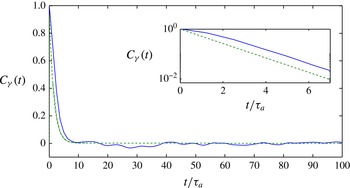
where the angle brackets denote the average over all particle pairs. As illustrated in figure 5,
 $C_{{\it\gamma}}(t)$
can be well approximated by an exponential function.
Lagrangian correlation of stretching rates
 ${\it\gamma}(t)$
. An exponential function
 $\text{e}^{-t/{\it\tau}_{c}}$
, with a correlation time
 ${\it\tau}_{c}=1.5{\it\tau}_{a}$
, is shown as a dashed line. The same curves are shown in a semi-logarithmic plot in the inset.

The PDF of elongation
 ${\it\rho}(t)$
in the following is denoted by
 $p_{{\it\rho}}({\it\rho},t)$
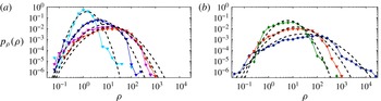
. As illustrated in figure 6(a),
 $p_{{\it\rho}}({\it\rho},t)$
has a significant probability of values less than one, which correspond to compression processes. Furthermore, its width increases with increasing time. As expected, increasing the degree of heterogeneity broadens the distribution of stretching rates shown in figure 6(b).
(a) PDF of elongations at times
 $t_{1}=0.25{\it\tau}_{a}$
,
 $t_{2}=12.5{\it\tau}_{a}$
,
 $t_{3}=50{\it\tau}_{a}$
and
 $t_{4}=112.5{\it\tau}_{a}$
, and (b) PDF of elongations at time
 $t_{4}=112.5{\it\tau}_{a}$
for
 ${\it\sigma}_{f}^{2}=0.25$
(diamonds),
 ${\it\sigma}_{f}^{2}=1$
(triangles),
 ${\it\sigma}_{f}^{2}=4$
(circles). The lognormal distributions predicted by (4.9) are shown by dashed lines with
 $\{{\it\mu}=0.55,{\it\nu}=0.1\}$
for
 ${\it\sigma}_{f}^{2}=0.25$
,
 $\{{\it\mu}=0.7,{\it\nu}=0.2\}$
for
 ${\it\sigma}_{f}^{2}=1$
and
 $\{{\it\mu}=1,{\it\nu}=0.35\}$
for
 ${\it\sigma}_{f}^{2}=4$
.

4.1. Non-linear stretching
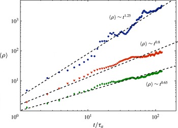
The average elongation is found, from our simulations, to be well fitted by a power law in time as
 $$\begin{eqnarray}\left\langle {\it\rho}(t)\right\rangle \propto \left(\frac{t}{{\it\tau}_{a}}\right)^{{\it\alpha}}.\end{eqnarray}$$
The profound nature of this behaviour and the origin of its connection with the structure of the permeability field are beyond the scope of the present work. We take (4.3) as an empirical fact, and note that the exponent
 ${\it\alpha}$
depends on the permeability field heterogeneity
 ${\it\sigma}_{f}^{2}$
, as illustrated in figure 7. Note that the power law behaviour does not hold at early times,
 $t<{\it\tau}_{a}$
, since the elongation
 ${\it\rho}$
should converge to one as time goes to zero. This non-linear stretching law has important implications for the geometry of the line. During its transport, the advected line is confined in a domain whose longitudinal extent grows as the advective spreading length
 ${\it\sigma}(t)$
and whose lateral extent is constant; see also figure 3.
Temporal evolution of the mean elongation
 $\langle {\it\rho}(t)\rangle$
for different permeability field variances:
 ${\it\sigma}_{\ln K}^{2}=0.25$
(diamonds),
 ${\it\sigma}_{\ln K}^{2}=1$
(triangles),
 ${\it\sigma}_{\ln K}^{2}=4$
(circles).

The advective spreading length
 ${\it\sigma}(t)$
is defined in terms of the longitudinal position of purely advectively transported particles
 $x_{1}(t)$
; this means that
 $D=0$
in (2.3), as
 $$\begin{eqnarray}{\it\sigma}^{2}(t)=\langle [x_{1}(t)-\langle x_{1}(t)\rangle ]^{2}\rangle .\end{eqnarray}$$
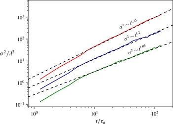
The angle brackets denote the average over all particles in the initial line. As shown in figure 8, the advective spatial variance increases non-linearly over the time scales of simulations, which is characteristic of non-Fickian spreading processes in heterogeneous media (Le Borgne et al.
Reference Le Borgne, Dentz and Carrera2008). The anomalous scaling of advective spreading is in general persistent in time as the advective sampling of the velocity heterogeneity is not fostered by diffusion. Hence, the convergence to Fickian advective dispersion is expected to occur at a characteristic advective time corresponding to the lowest velocity in the domain. This time may thus be very large for strongly heterogeneous media. Advective spreading in porous media has been shown to be characterized by strong intermittent properties, which can be related to the flow field heterogeneity by correlated continuous-time random walk approaches (de Anna et al.
Reference de Anna, Le Borgne, Dentz, Tartakovsky, Bolster and Davy2013). The non-linear evolution of the spatial variance
 ${\it\sigma}(t)$
in the non-Fickian regime is often approximated as a power law,
 $$\begin{eqnarray}{\it\sigma}(t)\propto t^{{\it\beta}/2},\end{eqnarray}$$
with
 $1\leqslant {\it\beta}\leqslant 2$
(figure 8).
Temporal evolution of the advective spatial variance
 ${\it\sigma}^{2}(t)$
, which characterizes advective spreading for
 ${\it\sigma}_{f}^{2}=0.25$
(green curve),
 ${\it\sigma}_{f}^{2}=1$
(blue curve) and
 ${\it\sigma}_{f}^{2}=4$
(red curve).

The power law evolution of the mean elongation
 $\langle {\it\rho}(t)\rangle$
and the advective spreading length
 ${\it\sigma}(t)$
implies that the advected line support is fractal, shown as follows. Considering a fractal line support, the number of boxes of size
 $r$
needed to cover the line at a line extension
 ${\it\sigma}(t)$
is
 $$\begin{eqnarray}N(r,t)\propto \left[\frac{r}{{\it\sigma}(t)}\right]^{-d_{f}}.\end{eqnarray}$$
Thus, with increasing time, the number of boxes of unit size needed to cover the line increases as
 ${\it\sigma}(t)^{d_{f}}$
. At the same time
 $N(r,t)$
increases according to
 $\langle {\it\rho}(t)\rangle$
so that
 $$\begin{eqnarray}\langle {\it\rho}(t)\rangle \propto {\it\sigma}(t)^{d_{f}}.\end{eqnarray}$$
Thus, since both
 $\langle {\it\rho}(t)\rangle$
and
 ${\it\sigma}(t)$
evolve as a power law of time, the line should be characterized by a stable fractal dimension
 $d_{f}$
such as
 $$\begin{eqnarray}d_{f}=\frac{2{\it\alpha}}{{\it\beta}}.\end{eqnarray}$$
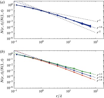
The fractal dimension of the advected line computed by box counting is found to be well defined over two orders of magnitude in space, as seen in figure 9 showing the number of boxes
 $N(r)\sim r^{-d_{f}}$
of size
 $r$
needed to cover the line support (Villermaux & Innocenti Reference Villermaux and Innocenti1999). It is independent of time and ranges from
 $d_{f}=1.3$
, for moderate heterogeneity, to
 $d_{f}=1.8$
, for strong heterogeneity, which is consistent with (4.8). Equation (4.8) thus provides a key relationship between stretching, spreading and the geometrical properties of the scalar field.
(a) Number of boxes
 $N(r)\sim r^{-d_{f}}$
of size
 $r$
needed to cover the line support (figure 3) at times
 $t_{1}=12.5{\it\tau}_{a}$
,
 $t_{2}=50{\it\tau}_{a}$
and
 $t_{3}=112.5{\it\tau}_{a}$
. (b) The same as (a) at time
 $t_{3}=112.5{\it\tau}_{a}$
for different permeability field heterogeneities:
 ${\it\sigma}_{f}^{2}=0.25$
(green curve),
 ${\it\sigma}_{f}^{2}=1$
(blue curve) and
 ${\it\sigma}_{f}^{2}=4$
(red curve).

4.2. Stochastic model of Lagrangian elongations
As discussed by Duplat et al. (Reference Duplat, Innocenti and Villermaux2010), different types of stochastic models can be considered for modelling stretching processes. The statistics of Lagrangian elongation suggests that the elongation process considered is characterized by relatively short-range correlated elongation rates
 ${\it\gamma}(t)$
, (4.1), as shown by the exponential decrease of the correlation of Lagrangian stretching rates (figure 5). Thus we model the fluctuations of
 ${\it\gamma}^{\prime }(t)$
as
 ${\it\gamma}^{\prime }(t)={\it\sigma}_{{\it\gamma}}(t){\it\xi}(t)$
with
 ${\it\xi}(t)$
a Gaussian white noise, which renders the evolution of
 ${\it\rho}(t)$
a multiplicative stochastic process through the definition of (4.1). Thus a simple stochastic model of Lagrangian elongation, which reflects the multiplicative nature of the stretching process, and satisfies the temporal power law behaviour of the mean elongation (4.3), established for
 $t>{\it\tau}_{a}$
, is the following Langevin equation (Le Borgne et al.
Reference Le Borgne, Dentz and Villermaux2013),
 $$\begin{eqnarray}\frac{1}{{\it\rho}}\frac{\text{d}{\it\rho}}{\text{d}t}=\frac{{\it\mu}}{t}+\sqrt{\frac{2{\it\nu}}{t}}\,{\it\xi}(t),\end{eqnarray}$$
where
 ${\it\xi}(t)$
is taken as a Gaussian white noise, with
 $\langle {\it\xi}(t)\rangle =0$
and
 $\langle {\it\xi}(t){\it\xi}(t^{\prime })\rangle ={\it\delta}(t-t^{\prime })$
, which results from the observed short-range temporal correlation of computed Lagrangian stretching rates
 ${\it\gamma}(t)$
seen in figure 4. Considering this equation in the Stratonovich interpretation (Risken Reference Risken1996), we obtain by integration of (4.9)
 $$\begin{eqnarray}{\it\rho}(t)=\left(\frac{t}{{\it\tau}_{a}}\right)^{{\it\mu}}\exp \!\left[\int _{{\it\tau}_{a}}^{t}\text{d}t^{\prime }\sqrt{\frac{2{\it\nu}}{t^{\prime }}}{\it\xi}(t^{\prime })\right]\end{eqnarray}$$
with the initial condition
 ${\it\rho}(t={\it\tau}_{a})=1$
. The mean and mean-squared elongations are given by
 $$\begin{eqnarray}\langle {\it\rho}(t)\rangle =\left(\frac{t}{{\it\tau}_{a}}\right)^{{\it\mu}+{\it\nu}},\quad \langle {\it\rho}(t)^{2}\rangle =\left(\frac{t}{{\it\tau}_{a}}\right)^{2{\it\mu}+4{\it\nu}}.\end{eqnarray}$$
Thus the exponent
 ${\it\alpha}$
in (4.3) can be expressed by
 ${\it\alpha}={\it\mu}+{\it\nu}$
. The parameters
 ${\it\mu}$
and
 ${\it\nu}$
are obtained from the numerically computed Lagrangian elongations as
 $\{{\it\mu}=0.6,{\it\nu}=0.05\}$
for
 ${\it\sigma}_{f}^{2}=0.25$
,
 $\{{\it\mu}=0.7,{\it\nu}=0.1\}$
for
 ${\it\sigma}_{f}^{2}=1$
, and
 $\{{\it\mu}=1.1,{\it\nu}=0.15\}$
for
 ${\it\sigma}_{f}^{2}=4$
.
The multiplicative noise structure of (4.9) implies that
 $z=\ln ({\it\rho})$
is normally distributed and therefore
 $p_{{\it\rho}}({\it\rho},t)$
is given by the lognormal distribution
 $$\begin{eqnarray}p_{{\it\rho}}({\it\rho},t)=\frac{1}{{\it\rho}}\frac{\exp \!\left\{-\displaystyle \frac{\left[\ln ({\it\rho})-{\it\mu}\ln (t/{\it\tau}_{a})\right]^{2}}{4{\it\nu}\ln (t/{\it\tau}_{a})}\right\}}{\sqrt{4{\rm\pi}{\it\nu}\ln (t/{\it\tau}_{a})}}.\end{eqnarray}$$
This agrees well with the elongation PDFs obtained numerically: see figure 6.
We can now determine the non-dimensional time
 ${\it\tau}(t)$
, (3.3), in terms of
 ${\it\rho}(t)$
. To this end, we note that the Langevin equation (4.9) may be written as
 $$\begin{eqnarray}\frac{\text{d}\ln ({\it\rho})}{\text{d}u}={\it\mu}+\sqrt{2{\it\nu}}\,{\it\xi}(u),\quad \frac{\text{d}\ln (t)}{\text{d}u}=1,\end{eqnarray}$$
which renders
 ${\it\rho}$
a function of
 $u=\ln (t)$
. Thus we can rewrite (3.3) for
 ${\it\tau}(t)$
as
 $$\begin{eqnarray}{\it\tau}(t)=\frac{D}{s_{0}^{2}}\int _{0}^{u}\text{d}u^{\prime }\exp (u^{\prime }){\it\rho}(u^{\prime })^{2}=\frac{D}{s_{0}^{2}}\int _{0}^{u}\text{d}u^{\prime }\exp [u^{\prime }+2\ln ({\it\rho})].\end{eqnarray}$$
Using (4.13) to express
 $\ln ({\it\rho})$
on the right-hand side, we obtain
 $$\begin{eqnarray}{\it\tau}(t)=\frac{D}{s_{0}^{2}}\int _{0}^{u}\text{d}u^{\prime }\exp \!\left[u^{\prime }+(2{\it\mu}+4{\it\nu})u^{\prime }\right]\,f(u^{\prime }),\end{eqnarray}$$
where
 $f(u^{\prime })=\exp [2\sqrt{2{\it\nu}}\int _{0}^{u^{\prime }}\text{d}y\,{\it\xi}(y)-4{\it\nu}u^{\prime }]$
. By a shift of the integration variable, the integral expression of
 ${\it\tau}(t)$
can be written as
 $$\begin{eqnarray}{\it\tau}(t)=\frac{D}{s_{0}^{2}}\exp [u(1+2{\it\mu}+4{\it\nu})]\int _{0}^{u}\text{d}u^{\prime }\exp [-u^{\prime }(1+2{\it\mu}+4{\it\nu})]\,f(u-u^{\prime }).\end{eqnarray}$$
The main contribution of the integrand comes from
 $u^{\prime }=0$
because the random function
 $f(u)>0$
is on average equal to 1 and its standard deviation goes as
 $\exp (4{\it\nu}u)$
. Thus we obtain approximately
 $$\begin{eqnarray}{\it\tau}(t)\approx \frac{D}{s_{0}^{2}}\frac{\exp [u(1+2{\it\mu}+4{\it\nu})]f(u)}{1+2{\it\mu}+4{\it\nu}}=\frac{D}{s_{0}^{2}}\frac{{\it\rho}(t)^{2}t}{1+2{\it\mu}+4{\it\nu}}.\end{eqnarray}$$
Using this approximation, the maximum lamella concentration
 ${\it\theta}(t)$
given by (3.4) can be related to the current lamella elongation as
 $$\begin{eqnarray}{\it\theta}(t)\approx {\it\rho}(t)^{-1}(At/{\it\tau}_{a})^{-1/2},\quad A=\frac{D{\it\tau}_{a}}{s_{0}^{2}c_{0}^{2}}\frac{4}{1+2{\it\mu}+4{\it\nu}},\end{eqnarray}$$
for
 ${\it\rho}(t)\gg 1$
. This scaling trivially expresses mass conservation in two dimensions, since at the lamella scale the product
 ${\it\theta}\sqrt{Dt}{\it\rho}$
remains constant in time. From (4.9), we obtain for
 ${\it\theta}(t)$
the evolution equation
 $$\begin{eqnarray}\frac{1}{{\it\theta}}\frac{\text{d}{\it\theta}}{\text{d}t}=-\frac{{\it\mu}}{t}-\frac{1}{2t}+\sqrt{\frac{2{\it\nu}}{t}}\,{\it\xi}(t),\end{eqnarray}$$
with
 ${\it\theta}(t={\it\tau}_{a})=A^{-1/2}\sim c_{0}$
. The PDF of
 ${\it\theta}(t)$
is lognormal,
 $$\begin{eqnarray}p_{{\it\theta}}({\it\theta},t)=\frac{\exp \!\left\{-\displaystyle \frac{[\ln ({\it\theta}/c_{0})-m_{z}]^{2}}{2{\it\sigma}_{z}^{2}}\right\}}{{\it\theta}\sqrt{2{\rm\pi}{\it\sigma}_{z}^{2}}},\end{eqnarray}$$
where
 $$\begin{eqnarray}m_{z}(t)=-{\it\mu}\ln (t/{\it\tau}_{a})-{\textstyle \frac{1}{2}}\ln (t/{\it\tau}_{a}),\quad {\it\sigma}_{z}^{2}(t)=2{\it\nu}\ln (t/{\it\tau}_{a})\end{eqnarray}$$
are the mean and variance of
 $z(t)=\ln [{\it\theta}(t)]$
. The moments of the maximum lamella concentration across the stretched lamellae are given by
 $$\begin{eqnarray}\langle {\it\theta}(t)^{q}\rangle =c_{0}^{q}\exp (qm_{z}+q^{2}{\it\sigma}_{z}^{2}/2)=c_{0}^{q}\left(\frac{t}{{\it\tau}_{a}}\right)^{-q{\it\mu}-(q/2)+q^{2}{\it\nu}}.\end{eqnarray}$$
A similar construction can be found in Kalda (Reference Kalda2000) and Meunier & Villermaux (Reference Meunier and Villermaux2010).
5. Mixing scale, mixing time
The derived model of Lagrangian elongations can be used to quantify the temporal evolution of the local mixing scale, whose evolution is governed by the competition between diffusive broadening and substrate compression perpendicular to the elongation direction (Le Borgne et al.
Reference Le Borgne, Dentz, Davy, Bolster, Carrera, de Dreuzy and Bour2011; Villermaux Reference Villermaux2012). These two effects equilibrate at the mixing time, when the transverse lamellae thickness has reached the Batchelor scale (Batchelor Reference Batchelor1959). This competition is expressed by the advection–diffusion equation (3.1). The local scale
 ${\it\epsilon}_{m}(t)$
is defined from the variance of the concentration profile across a lamella (Villermaux Reference Villermaux2012) as a measure of the lamellae ‘thickness’,
 ${\it\epsilon}_{m}^{2}(t)=\int \!\text{d}{\it\zeta}\,{\it\zeta}^{2}c({\it\zeta},t)/\!\int \!\text{d}{\it\zeta}\,c({\it\zeta},t)$
. Using expression (3.2) for
 $c({\it\zeta},t)$
, we have
 ${\it\epsilon}_{m}^{2}(t)=s_{0}^{2}/(2{\it\rho}(t)^{2})+(2s_{0}^{2}{\it\tau}(t))/({\it\rho}(t)^{2})$
. Further using approximation (4.17) for
 ${\it\tau}(t)$
yields
 $$\begin{eqnarray}{\it\epsilon}_{m}^{2}(t)=\frac{s_{0}^{2}}{2{\it\rho}(t)^{2}}+\frac{2Dt}{1+2{\it\mu}+4{\it\nu}}.\end{eqnarray}$$
Note that the elongation
 ${\it\rho}(t)$
is lognormally distributed and given by (4.12). We obtain for the evolution of the average mixing scale
 $s_{m}(t)=\langle {\it\epsilon}_{m}(t)\rangle$
from (5.1) the approximate expression
 $$\begin{eqnarray}s_{m}(t)\approx \sqrt{\frac{s_{0}^{2}}{2}\left(\frac{t}{{\it\tau}_{a}}\right)^{-2{\it\mu}+2{\it\nu}}+\frac{2Dt}{1+2{\it\mu}+4{\it\nu}}}.\end{eqnarray}$$
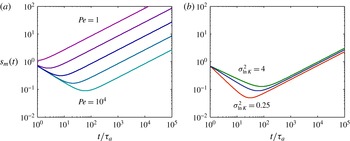
Figure 10 shows the temporal evolution of the average mixing scale for different Péclet numbers and permeability field variances. Since the compression rate is stronger than diffusive growth at early times, the mixing scale
 $s_{m}$
decays until it reaches the Bachelor scale at which the diffusive growth balances compressive effects due to stretching. This occurs at the mixing time
 ${\it\tau}_{m}$
for which
 $$\begin{eqnarray}\frac{\text{d}s_{m}({\it\tau}_{m})}{\text{d}t}=0,\quad \frac{{\it\tau}_{m}}{{\it\tau}_{a}}\propto \mathit{Pe}_{0}^{1/(1+2{\it\mu}-2{\it\nu})},\end{eqnarray}$$
where we have defined the strip Péclet number
 $\mathit{Pe}_{0}=s_{0}^{2}/{\it\tau}_{a}D$
. The ratio between the mixing time
 ${\it\tau}_{m}$
and the diffusion time
 ${\it\tau}_{D}$
can be expressed as
 ${\it\tau}_{m}/{\it\tau}_{D}=(s_{0}/{\it\lambda})^{2/(1+2{\it\mu}-2{\it\nu})}\mathit{Pe}^{-(2{\it\mu}-2{\it\nu})/(1+2{\it\mu}-2{\it\nu})}$
. Since the exponent
 $-(2{\it\mu}-2{\it\nu})/(1+2{\it\mu}-2{\it\nu})$
is negative, the difference between
 ${\it\tau}_{m}$
and
 ${\it\tau}_{D}$
is expected to increase with Péclet number. For large Péclet numbers
 $\mathit{Pe}\gg 1$
, the mixing time occurs long before the diffusion time. On the other hand, for small Péclet numbers
 $\mathit{Pe}\ll 1$
, the diffusion time may occur before the mixing time. In this case, we expect stretching to have a minor effect on the concentration field, as diffusion would be the dominating process.
Temporal evolution of the average mixing scale (5.2), (a) for different Péclet numbers
 $\mathit{Pe}=1$
, 10,
 $10^{2}$
,
 $10^{3}$
,
 $10^{4}$
and
 ${\it\sigma}_{\ln K}^{2}=1$
, and (b) for different permeability field variances
 ${\it\sigma}_{\ln K}^{2}=0.25$
, 1, 4 and
 $\mathit{Pe}=10^{4}$
.

The mixing scale at time
 ${\it\tau}_{m}$
defines the Batchelor scale
 $s_{B}=s_{m}({\it\tau}_{m})$
, given by
 $$\begin{eqnarray}\frac{s_{B}}{s_{0}}\propto {\mathit{Pe}_{0}}^{(2{\it\nu}-{\it\mu})/(1+2{\it\mu}-2{\it\nu})}.\end{eqnarray}$$
Before the mixing time, the decay of the average mixing scale is controlled by the elongation process,
 $s_{m}\sim \langle {\it\rho}\rangle ^{-1}\sim t^{-{\it\mu}-{\it\nu}}$
, which depends on the permeability field heterogeneity (figure 10
b). After the mixing time, the average mixing scale grows as
 $s_{m}=\sqrt{(2Dt)/(1+2{\it\mu}+4{\it\nu})}$
for all degrees of heterogeneity.
The explicit relation (5.1) between the mixing scale
 ${\it\epsilon}_{m}(t)$
and the elongation
 ${\it\rho}(t)$
allows us to derive the PDF of
 ${\it\epsilon}_{m}(t)$
by mapping from the PDF (4.12) of
 ${\it\rho}(t)$
. Thus we obtain the shifted lognormal PDF
 $$\begin{eqnarray}p_{{\it\epsilon}_{m}}({\it\epsilon}_{m},t)=\frac{{\it\epsilon}_{m}\exp \!\left\{-\displaystyle \frac{\left[\ln \left({\it\epsilon}_{m}^{2}\displaystyle -\frac{2Dt}{1+2{\it\mu}+4{\it\nu}}\right)-\ln (s_{0}^{2}/2)+2{\it\mu}\ln (t/{\it\tau}_{a})\right]^{2}}{16{\it\nu}\ln (t/{\it\tau}_{a})}\right\}}{[{\it\epsilon}_{m}^{2}-2Dt/(1+2{\it\mu}+4{\it\nu})]\sqrt{4{\rm\pi}{\it\nu}\ln (t/{\it\tau}_{a})}},\end{eqnarray}$$
for
 ${\it\epsilon}_{m}\geqslant \sqrt{(2Dt)/(1+2{\it\mu}+4{\it\nu})}$
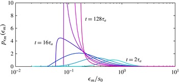
and zero otherwise. This lower limit corresponds to the most stretched fraction of lamellae which have attained their mixing time and are growing diffusively. The temporal evolution of the mixing scale PDF is illustrated in figure 11 for
 $\mathit{Pe}=10^{4}$
. At early times, the distribution of mixing scales is broad, reflecting the broad distribution of stretching rates and line elongation. With increasing time, the peak of the PDF moves towards smaller values of
 ${\it\epsilon}_{m}$
as a consequence of lamella compression. For times larger than the mixing time
 ${\it\tau}_{m}$
, diffusion wins over compression in the evolution of the mixing scale,
 ${\it\epsilon}_{m}=\sqrt{(2Dt)/(1+2{\it\mu}+4{\it\nu})}$
. The random nature of the stretching process has only a marginal influence on the mixing scale, which now evolves deterministically. Therefore the PDF
 $p_{{\it\epsilon}_{m}}({\it\epsilon}_{m})$
converges asymptotically to a Dirac-delta distribution
 $$\begin{eqnarray}p_{{\it\epsilon}_{m}}({\it\epsilon}_{m})={\it\delta}\left({\it\epsilon}_{m}-\sqrt{\frac{2Dt}{1+2{\it\mu}+4{\it\nu}}}\right),\end{eqnarray}$$
expressing the fact that all lamellae ultimately experience the same history, because they have sampled the space of possible stretching values.
PDF of mixing scales
 $p_{{\it\epsilon}_{m}}({\it\epsilon}_{m})$
for
 $\mathit{Pe}=10^{4}$
at times
 $t=2{\it\tau}_{a}$
,
 $4{\it\tau}_{a}$
,
 $8{\it\tau}_{a}$
,
 $16{\it\tau}_{a}$
,
 $32{\it\tau}_{a}$
,
 $64{\it\tau}_{a}$
,
 $128{\it\tau}_{a}$
.

6. Concentration PDF of an ensemble of non-interacting lamellae
For large Péclet numbers, a well-developed regime exists in which lamellae do not overlap, as illustrated in figure 1(b). We describe here a corresponding mixing model which maps the PDF of lamella elongations into the PDF of concentrations. The predictions are compared to the concentration data of the full flow and transport simulations.
In this regime, the concentration PDF
 $p_{c}(c,t)$
is obtained by sampling concentration over individual lamellae, whose PDF (3.5) is conditional to the respective maximum concentration
 ${\it\theta}(t)$
. The maximum concentration describes a stochastic process due to the stochasticity of the elongation
 ${\it\rho}(t)$
. The PDF of
 ${\it\theta}(t)$
is denoted by
 $p_{{\it\theta}}({\it\theta},t)$
. The concentration PDF is thus written as
 $$\begin{eqnarray}p_{c}(c,t)=\int _{c}^{\infty }\text{d}{\it\theta}\,p_{c}(c|{\it\theta})p_{{\it\theta}}({\it\theta},t).\end{eqnarray}$$
Using (4.20) in (6.1) and rescaling the integration variable, we can write the concentration PDF as
 $$\begin{eqnarray}p_{c}(c,t)=\int _{\ln (c)}^{\infty }\text{d}z\frac{\exp \!\left[-\displaystyle \frac{(z-m_{z})^{2}}{2{\it\sigma}_{z}^{2}}\right]}{2c\sqrt{2{\rm\pi}{\it\sigma}_{z}^{2}}\sqrt{[z-\ln ({\it\epsilon})][z-\ln (c)]}},\end{eqnarray}$$
where we used (3.5) for
 $p_{c}(c|{\it\theta})$
. For concentrations
 $\ln (c)<m_{z}$
, the PDF can be approximated by
 $$\begin{eqnarray}p_{c}(c,t)\approx \frac{1}{2c\sqrt{[m_{z}-\ln ({\it\epsilon})][m_{z}-\ln (c)]}},\end{eqnarray}$$
thus exhibiting the
 $1/c$
-decay characteristic for the diffusive profile (3.5) across the lamella. For concentrations
 $\ln (c)>m_{z}$
, we obtain the approximation
 $$\begin{eqnarray}p_{c}(c,t)\approx \frac{\exp \!\left\{-\displaystyle \frac{[\ln (c)-m_{z}]^{2}}{2{\it\sigma}_{z}^{2}}\right\}}{c\sqrt{8\ln (c/{\it\epsilon})[\ln (c)-m_{z}]}}.\end{eqnarray}$$
For large concentrations, the PDF decreases essentially as the lognormal distribution.
The concentration PDF (6.2) is parametrized only by the parameters
 ${\it\mu}$
and
 ${\it\nu}$
in (4.9), which are obtained from the evolution of
 ${\it\rho}(t)$
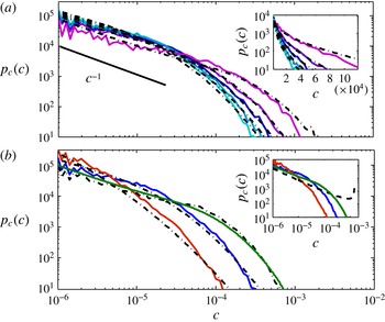
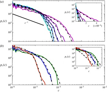
. Its predictions are in good agreement with the numerical simulations for all cases, in which the stretched lamellae that constitute the line evolve on their own and do not overlap, i.e. at early times and high Péclet numbers (this is illustrated in figure 12). The model predicts correctly the temporal evolution of the shape of the concentration PDF, as it evolves towards uniformity.
(a) Concentration PDFs at times
 $t=12.5{\it\tau}_{a}$
,
 $37.5{\it\tau}_{a}$
,
 $62.5{\it\tau}_{a}$
,
 $87.5{\it\tau}_{a}$
,
 $112.5{\it\tau}_{a}$
for a Péclet number
 $\mathit{Pe}=8\times 10^{4}$
and a permeability field variance
 ${\it\sigma}_{f}^{2}=1$
. The simulations are represented by solid lines and the predictions obtained from the independent lamella model (6.2) are represented by dot-dashed lines. The inset shows the same plot in semi-log representation, emphasizing the non-exponential concentration decay. (b) Concentration PDFs at time
 $112.5{\it\tau}_{a}$
for a Péclet number
 $\mathit{Pe}=8\times 10^{4}$
and permeability field variances of
 ${\it\sigma}_{f}^{2}=0.25$
(green line),
 ${\it\sigma}_{f}^{2}=1$
(blue line) and
 ${\it\sigma}_{f}^{2}=4$
(red line). The predictions obtained from the independent lamella model (6.2) are represented by dot-dashed lines. The inset shows the prediction of the purely diffusive model (3.5), with
 ${\it\theta}=c_{0}/\sqrt{4{\rm\pi}Dt}$
.

The behaviour of
 $p_{c}(c,t)$
for small concentrations is given by
 $p_{c}\propto 1/[c\sqrt{\ln (1/c)}]$
, which is characteristic of the Gaussian concentration profiles across each lamella as given in (3.2). The PDF of large concentrations is controlled by the lognormal PDF of maximum lamella concentrations
 $p_{m}({\it\theta})$
, as expressed by (6.4). Comparison with the prediction of a purely diffusive model (inset of figure 12
b) shows that flow heterogeneity considerably accelerates the temporal decay of concentration levels via stretching-enhanced diffusive mixing. Furthermore, the model predicts accurately the impact of heterogeneity on mixing and represents well the decrease of the maximum concentration as the degree of heterogeneity increases. This is illustrated in figure 12(b).
A corresponding similar example of broad concentration statistics reflecting only the distributed histories among non-interacting lamellae is provided by mixing in the dispersing turbulent plume studied by Duplat et al. (Reference Duplat, Innocenti and Villermaux2010).
7. Concentration PDF of an ensemble of interacting lamellae
Interactions between lamellae are enforced at later times and for smaller Péclet numbers because the average elongation
 $\langle {\it\rho}\rangle \propto t^{{\it\alpha}}$
grows faster than the longitudinal size of the dispersion area
 ${\it\sigma}\propto t^{{\it\alpha}/d_{f}}$
in which the line is confined. Recall that
 $d_{f}\geqslant 1$
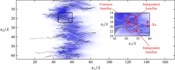
as given in (4.8). When the lamella width is larger than the distance between lamellae, the concentration fields around each lamella start coalescing to form lamella aggregates, as illustrated in figure 13. Due to continued diffusive broadening these lamella aggregates may overlap to form bundles. We develop here a mixing theory in which lamella interaction is modelled as a random aggregation process with partial or complete coalescence. The coalescence processes and model predictions are tested by comparison to detailed numerical simulations.
Concentration field and advected line at time
 $t=112.5{\it\tau}_{a}$
and for a Péclet number
 $\mathit{Pe}=800$
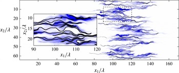
. The inset illustrates the concentration build-up in areas with a large density of lamellae.

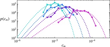
PDF of local maximum concentrations
 $p(c_{m},t)$
, Péclet number
 $\mathit{Pe}=80$
. The PDF is plotted for times
 $t_{1}=12.5{\it\tau}_{a}$
(triangles),
 $t_{2}=37.5{\it\tau}_{a}$
(diamonds),
 $t_{3}=62.5{\it\tau}_{a}$
(squares) and
 $t_{4}=112.5{\it\tau}_{a}$
(circles). The dashed lines represent the prediction of the Gamma distribution (7.1) for an average number of overlaps obtained from (7.9).

7.1. Concentration PDF of lamella aggregates
This process can be described by the random aggregation process proposed in Villermaux & Duplat (Reference Villermaux and Duplat2003). We consider an aggregate of
 $n$
lamellae, characterized by the maximum concentration
 $c_{m}$
. The value of
 $c_{m}$
results from the addition of concentration levels of the individual lamellae. Assuming that the lamellae that overlap have uncorrelated stretching histories, these concentration levels can be considered as uncorrelated random variables, and the coalescence can be described as a random aggregation process (e.g. Villermaux & Duplat Reference Villermaux and Duplat2003). The concentration PDF
 $p_{m}[c_{m},t|n]$
is then given by a Gamma distribution of order
 $n$
, independent of the initial distribution,
 $$\begin{eqnarray}p_{m}(c_{m},t|n)=\frac{c_{m}^{n-1}}{\langle {\it\theta}(t)\rangle ^{n}{\rm\Gamma}(n)}\exp \!\left[-\frac{c_{m}}{\langle {\it\theta}(t)\rangle }\right],\end{eqnarray}$$
where
 $\langle {\it\theta}(t)\rangle$
is the average concentration of an elementary lamella at time
 $t$
given by (4.22) for
 $q=1$
, which derives from the stretching-enhanced diffusive regime described earlier.
We approximate the concentration profile around each aggregate by a Gaussian spatial profile. Thus the concentration PDF
 $p_{c}(c|c_{m})$
conditioned on the maximum concentration
 $c_{m}$
is given by (3.5). The concentration PDF across lamella aggregates containing
 $n(t)$
lamellae is then given by
 $$\begin{eqnarray}p_{c}(c,t|n)=\int _{c}^{c_{0}}\text{d}c_{m}\frac{c_{m}^{n-1}}{\langle {\it\theta}(t)\rangle ^{n}{\rm\Gamma}[n]}\frac{\exp \!\left[-\displaystyle \frac{c_{m}}{\langle {\it\theta}(t)\rangle }\right]}{2c\sqrt{\ln (c_{m}/{\it\epsilon})\ln (c_{m}/c)}},\end{eqnarray}$$
for
 $c\geqslant {\it\epsilon}$
.
To test the validity of (7.1), we evaluate numerically the PDF of local concentration maxima. To do so, we compute the PDF
 $p_{m}(c_{m},x_{1},t)$
of concentration maxima at positions
 $x_{1}$
along the mean flow by sampling concentration values along
 $x_{2}$
, the direction perpendicular to the mean flow. The PDF of concentration maxima
 $p_{m}(c_{m},t)$
is then obtained by averaging
 $p_{m}(c_{m},x_{1},t)$
over
 $x_{1}$
. Figure 14 shows the resulting concentration PDF
 $p_{m}(c_{m},t)$
. The distribution of local maxima narrows down with time, following the characteristic shape of the Gamma distribution. The prediction of (7.1) is in good agreement with the numerical simulations. The Gamma distribution of local concentration maxima thus supports the random addition nature of the lamella aggregation process. In order to obtain an estimate for the distribution of local maxima from (7.1), we require the number of lamellae across bundles
 $n$
. We set the number of lamellae equal to the average number of lamellae
 $\langle n\rangle$
across bundles. In general, the number of lamellae is dependent on the position
 $x_{1}$
at which the cross-section is taken. This is discussed in the following section.
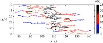
Illustration of the method used to estimate the number of overlaps along the line
 $n[\boldsymbol{x}(t|\boldsymbol{b}),r,t]$
for a diffusion scale
 $r=4{\it\lambda}$
at time
 $t=112,5{\it\tau}_{a}$
.

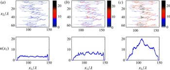
(a–c) Map of the number of overlaps
 $n[\boldsymbol{x}(t|\boldsymbol{b}),r,t]$
along the line for (a)
 $r={\it\lambda}/4$
, (b)
 $r={\it\lambda}$
and (c)
 $r=4{\it\lambda}$
at time
 $t=112,5{\it\tau}_{a}$
. (d–f) Projection of the number of overlaps as a function of the longitudinal position
 $n(x_{1},r,t)$
for each case.

7.2. Analysis of the distribution of lamella overlaps
The number of lamellae
 $n[\boldsymbol{x}(t|b),r,t]$
within a radius
 $r$
around the position
 $\boldsymbol{x}(t|b)$
in the purely advectively transported line is obtained by counting all particles at locations
 $\boldsymbol{x}(t|a)$
in the line that are within a radius
 $r$
and subsequent normalization by
 $r$
, as illustrated in figure 15. Note that
 $\boldsymbol{x}(t|a)$
is the trajectory of a purely advectively transported particle, i.e.
 $D=0$
in (2.3). The initial particle distribution is a uniform line at
 $x_{1}(t=0|a)={\it\lambda}$
and
 $x_{2}(t=0|a)=a$
. Note also that the number of particles within a radius
 $r$
of the position
 $\boldsymbol{x}(t|b)$
includes the particles inside the same lamella, whose number increases according to
 $r$
. The normalization by
 $r$
corrects for this. Figure 16 shows maps of
 $n[\boldsymbol{x}(t|b),r,t]$
along the stretched and folded line, as well as the projection of the number of lamellae
 $n(x_{1},r,t)$
at a position
 $x_{1}$
along the mean flow direction at time
 $t=112.5{\it\tau}_{a}$
and for
 $r={\it\lambda}/4$
,
 ${\it\lambda}$
and
 $4{\it\lambda}$
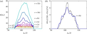
. The number of overlaps is distributed along the line with large overlap numbers in regions of high lamellae density, where the line is folded several times over itself. For small
 $r$
(see figure 16
a), the number of overlaps
 $n(x_{1},r,t)$
is found to be approximately constant along the longitudinal direction. When
 $r$
reaches the characteristic heterogeneity length
 ${\it\lambda}$
, the number of overlaps increases drastically at the centre of the plume, as illustrated in figures 16(b) and 17(c).
(a) Projection of the number of overlaps as a function of the longitudinal position
 $n(x_{1},r,t)$
for
 $r={\it\lambda}/4$
to
 $r=32{\it\lambda}$
. (b) Comparison of
 $n(x_{1},r,t)/\overline{n}(r,t)$
and
 $c_{a}(x,t)$
for
 $r=8{\it\lambda}$
.

This phenomenon can be seen as a percolation process (Villermaux Reference Villermaux2012). While for small
 $r$
lamella aggregates are isolated from each other, they become connected with increasing
 $r$
to form lamella bundles. This process is most active at the centre of the plume where the density of lamellae tends to be larger. The transition to percolation occurs approximately at
 $r={\it\lambda}$
. Note that lamellae within a radius
 $r$
coalesce only if the lamella width (5.1) is equal to
 $r$
. This means for the present regime that
 $r\approx \sqrt{Dt}$
. Thus percolation occurs at the characteristic diffusion time
 ${\it\tau}_{D}={\it\lambda}^{2}/D$
.
For
 $r>{\it\lambda}$
, i.e. at times
 $t>{\it\tau}_{D}$
,
 $n(x_{1},r,t)$
follows a distribution which peaks at the centre of the plume and sharply reduces with distance from the peak position: see figure 17(a). In this regime, the projected density of purely advectively transported particles
 $c_{a}(x_{1},t)$
is proportional to the density
 $n(x_{1},r,t)$
of lamellae at
 $x_{1}$
,
 $c_{a}(x_{1},t)\approx n(x_{1},r,t)/\overline{n}(r,t)$
, with
 $\overline{n}(r,t)$
the average number of lamellae within a radius
 $r$
. Thus we obtain for
 $n(x_{1},r,t)$
the approximation
 $$\begin{eqnarray}n(x_{1},r,t)\approx \overline{n}(r,t)c_{a}(x_{1},t).\end{eqnarray}$$
Figure 17(b) compares
 $n(x_{1},r,t)/\overline{n}(r,t)$
and
 $c_{a}(x_{1},t)$
at time
 $t=112,5{\it\tau}_{a}$
, and confirms (7.3).
The PDF
 $p_{n}(n,t,r)$
of the number of lamellae in the time regime
 $t>{\it\tau}_{D}$
can be estimated as
 $$\begin{eqnarray}p_{n}(n,t,r)=\left|\frac{\text{d}x_{1}(c_{a})}{\text{d}c_{a}}\right|_{c_{a}=n/\overline{n}(r,t)}.\end{eqnarray}$$
The longitudinal concentration distribution
 $c_{a}(x_{1},t)$
is often approximated by a Gaussian distribution in the Fickian dispersion framework. However, for the purely advective case, the upstream and downstream tails are determined respectively by the minimum and maximum velocities. Thus the longitudinal concentration distribution does not present infinite tails, as does the Gaussian distribution. In fact, according to figure 17(b), we approximate
 $c_{a}(x,t)$
by a linear distribution with
 $|\text{d}x(c_{a})/\text{d}c_{a}|=\text{const}$
. Thus for
 $t>{\it\tau}_{D}$
,
 $p_{n}(n,t,r)$
is given by the uniform distribution
 $$\begin{eqnarray}p_{n}(n,r,t)=\frac{1}{2\overline{n}(r,t)}\end{eqnarray}$$
for
 $0\leqslant n<2\overline{n}(r,t)$
. For times
 $t<{\it\tau}_{D}$
, the spatial profile of
 $n(x_{1},r,t)$
is uniform and thus the PDF
 $p_{n}(n,t,r)$
can be approximated by the delta density
 $$\begin{eqnarray}p_{n}(n,t,r)={\it\delta}[n-\overline{n}(r,t)].\end{eqnarray}$$
7.3. Temporal evolution of the average number of lamella overlaps
The average number
 $\overline{n}(r,t)$
of lamellae with concentration
 $\langle {\it\theta}(t)\rangle$
having coalesced in a radius
 $r$
is such that it restores, by addition, the average mixture concentration
 $\langle c(\boldsymbol{x},t)\rangle$
so that
 $$\begin{eqnarray}\langle c(\boldsymbol{x},t)\rangle =\overline{n}(r,t)\langle {\it\theta}(t)\rangle .\end{eqnarray}$$
For times below the percolation threshold
 $t<{\it\tau}_{D}$
, the number of lamellae within a radius
 $r$
is conditioned by the geometry of the folded and stretched line support. In order to determine the number of lamellae
 $\overline{n}(r,t)$
, we consider the number
 $n_{p}(r,t)$
of particle pairs in the purely advectively transported line that are separated by a distance smaller than
 $r$
. Thus the number of lamellae within a radius
 $r$
is given by
 $\overline{n}(r,t)=n_{p}(r,t)/r$
, where the normalization by
 $r$
is done to correct for the particles which belong to the same lamella as in the previous section. The number of particle pairs
 $n_{p}(r,t)$
over a fractal support scales as
 $n_{p}(r,t)\sim r^{d_{f}}$
, where
 $d_{f}$
is the fractal dimension of the line support (Grassberger & Procaccia Reference Grassberger and Procaccia1983). Therefore the average of lamella overlaps behaves as
 $$\begin{eqnarray}\overline{n}(r,t)\sim r^{d_{f}-1}.\end{eqnarray}$$
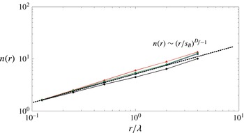
Hence, the average number of lamella overlaps is determined by the fractal dimension of the line support, which is set by the stretching and spreading dynamics via (4.8). This spatial scaling is consistent with numerical estimates (figure 18).
Average number of overlaps
 $\overline{n}(r,t)$
for times
 $t_{1}=12.5{\it\tau}_{a}$
(triangles),
 $t_{2}=37.5{\it\tau}_{a}$
(diamonds),
 $t_{3}=62.5{\it\tau}_{a}$
(squares) and
 $t_{4}=112.5{\it\tau}_{a}$
(circles). The dashed line represents the prediction of (7.9).

Compression perpendicular to the direction of elongation implies that lamellae may approach each other as close as the Batchelor scale in (5.4). Hence, the first lamella overlap is expected to occur at the mixing time, when diffusive growth overcomes compression. Thus, at
 $t={\it\tau}_{m}$
and
 $r=s_{B}$
((5.3) and (5.4)), the number of overlaps is expected to be on average equal to one. After the mixing time, the width of the diffusive profile of a single lamella (5.1) increases like
 $\sqrt{Dt}$
, which sets
 $r$
. Thus, for the temporal evolution of the mean number of coalescing lamellae, we obtain
 $$\begin{eqnarray}\overline{n}_{c}(t)=\left(Dt/s_{B}^{2}\right)^{(d_{f}-1)/2},\quad \text{for }{\it\tau}_{m}<t<{\it\tau}_{D}.\end{eqnarray}$$
The mixing time
 ${\it\tau}_{m}$
(5.3) sets the characteristic time for the transition from stretching-enhanced mixing to lamella coalescence. Note that the time range
 ${\it\tau}_{m}<t<{\it\tau}_{D}$
spans two orders of magnitude for
 $\mathit{Pe}=8$
and four orders of magnitude for
 $\mathit{Pe}=8\times 10^{4}$
. Hence, over this range of time scales, we expect the concentration field to be composed of aggregates of coalesced lamellae in areas where the line is densely folded over itself, and concentration lacunarities in low-flow zones which have not been filled by diffusion.
For times above the percolation threshold
 $t>{\it\tau}_{D}$
, most of the concentration lacunarities have been filled at the centre of the plume. Hence, the average concentration in the plume is estimated from the longitudinal plume extension
 ${\it\sigma}$
as
 $\langle c\rangle \propto 1/{\it\sigma}$
. Thus, in this regime, the average number of coalescences that restores the average concentration is obtained from (7.7) as
 $$\begin{eqnarray}\overline{n}_{c}(t)\propto \frac{1}{{\it\sigma}(t)\left\langle {\it\theta}(t)\right\rangle },\quad \text{for }t>{\it\tau}_{D}.\end{eqnarray}$$
7.4. Concentration PDF
The overall concentration PDF depends on the PDF of the number of lamellae in a given distance
 $r$
(7.4). The density of lamella coalescences at a given time
 $t$
is obtained by setting
 $r=\sqrt{2Dt}$
and substituting
 $\overline{n}(r,t)$
by
 $\overline{n}_{c}(t)$
in (7.5) and (7.6).
7.5. Partial coalescence regime
For
 ${\it\tau}_{m}<t<{\it\tau}_{D}$
, the number of overlaps is approximately constant along the line and the density of lamellae is such that it allows an essentially diffusive concentration profile within the aggregate. Thus the concentration PDF is obtained by setting
 $n=\overline{n}_{c}(t)$
in (7.2) as
 $$\begin{eqnarray}p_{c}(c,t)=\int _{c}^{c_{0}}\text{d}c_{m}\frac{c_{m}^{\overline{n}_{c}-1}}{\langle {\it\theta}\rangle ^{\overline{n}_{c}}{\rm\Gamma}(\overline{n}_{c})}\frac{\exp (-c_{m}/\langle {\it\theta}\rangle )}{2c\sqrt{\ln (c_{m}/{\it\epsilon})\ln (c_{m}/c)}},\end{eqnarray}$$
with
 $\overline{n}_{c}$
given by (7.9). For concentration
 $c<\overline{n}_{c}\langle {\it\theta}\rangle$
, we can approximate the PDF (7.11) by
 $$\begin{eqnarray}p_{c}(c,t)\approx \frac{1}{2c\sqrt{\ln [(\overline{n}_{c}-1)\langle {\it\theta}\rangle /{\it\epsilon}]\ln [(\overline{n}_{c}-1)\langle {\it\theta}\rangle /c]}}.\end{eqnarray}$$
Thus, for small concentrations, the PDF is dominated by the diffusive concentration profile that persists in the gaps between the lamella aggregates. For
 $c>\overline{n}_{c}\langle {\it\theta}\rangle$
, i.e. for larger concentrations, the PDF (7.11) behaves as
 $$\begin{eqnarray}p_{c}(c,t)\approx \frac{c^{\overline{n}_{c}-1}}{2\langle {\it\theta}\rangle ^{\overline{n}_{c}}{\rm\Gamma}(\overline{n}_{c})}\frac{\exp (-c/\langle {\it\theta}\rangle )}{\sqrt{\ln (c/{\it\epsilon})}}\frac{\sqrt{{\rm\pi}}}{\sqrt{c/\langle {\it\theta}\rangle -(\overline{n}_{c}-1)}},\end{eqnarray}$$
with a large-concentration exponential decay characteristic of the Gamma distribution.
The prediction of (7.11) for the temporal evolution of the concentration PDF is found to be in good agreement with the numerical simulations, as illustrated in figure 19. In particular, the large concentration behaviour of the PDF shows the exponential decay described in (7.13) (see inset of figure 19 a). This property, which is not observed in the first regime when the line does not interact with itself (see inset of figure 12 a), is a characteristic of the coalescence process described by (7.1). As outlined above, the low concentration behaviour (7.12) results from the diffusive profiles around the lamella aggregates. The comparison with the prediction of (6.2) (see inset of figure 19 b), which does not account for lamella interactions, shows that the coalescence process tends to increase the intermediate concentration probabilities around the average at the expense of the probability of high and low concentration levels.
(a) Concentration PDFs at times
 $t=12.5{\it\tau}_{a}$
,
 $37.5{\it\tau}_{a}$
,
 $62.5{\it\tau}_{a}$
,
 $87.5{\it\tau}_{a}$
,
 $112.5{\it\tau}_{a}$
for a Péclet number
 $\mathit{Pe}=8\times 10^{2}$
and a permeability field variance
 ${\it\sigma}_{\ln K}^{2}=1$
(solid lines). The predictions of the coalescence model (7.11) are shown by dot-dashed lines. The inset displays the same graph in semi-log representation, showing the exponential decay of the concentration PDFs in this regime. (b) Concentration PDFs for different permeability variances,
 ${\it\sigma}_{\ln K}^{2}=0.25$
(green line),
 ${\it\sigma}_{\ln K}^{2}=1$
(blue line) and
 ${\it\sigma}_{\ln K}^{2}=4$
(red line), at time
 $112.5{\it\tau}_{a}$
for a Péclet number
 $\mathit{Pe}=8\times 10^{2}$
. The predictions of the coalescence model (7.11) are shown by dot-dashed lines. The inset shows the predictions of the model of non-interacting lamellae (6.2) as dashed lines. In this regime the coalescence of lamellae tends to increase the probability of occurrence of intermediate concentrations.

7.6. Percolating coalescence regime
For
 $t>{\it\tau}_{D}$
, the concentration field is composed of bundles of aggregated lamellae, whose number varies along the mean flow direction according to (7.5). Aggregates with a number of lamellae that is smaller than or equal to
 $\overline{n}_{c}({\it\tau}_{D})=({\it\lambda}/s_{B})^{d_{f}-1}$
(see (7.9)) are characterized by a diffusive profile across the aggregate and thus the concentration PDF is given by
 $p_{c}(c,t|n)$
(see (7.2)). For
 $n>\overline{n}_{c}({\it\tau}_{D})$
, this means that, above the percolation threshold, the lamella density in the aggregate is so large that there is no space for a diffusive profile to develop between lamellae, and therefore the concentration PDF is given by the PDF (7.1) of concentration maxima
 $p_{m}(c,t|n)$
with
 $n=\overline{n}_{c}(t)$
given by (7.10),
 $$\begin{eqnarray}p_{c}(c,t)=\frac{c^{\overline{n}_{c}-1}}{\langle {\it\theta}\rangle ^{\overline{n}_{c}}{\rm\Gamma}(\overline{n}_{c})}\exp (-c/\langle {\it\theta}\rangle ).\end{eqnarray}$$
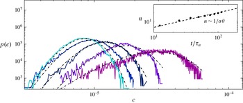
We expect this distribution of concentration values around the centre of the plume because there the lamella density is highest: see figure 16. This prediction is verified in figure 20, where the concentration PDF is computed at the centre of the plume for a Péclet number
 $\mathit{Pe}=8$
at different times. In order to analyse the concentration PDF in a region where full percolation occurs, we evaluate the concentration statistics at the central longitudinal positions
 $x$
, defined by
 $\overline{x_{1}}(x_{2})-{\it\sigma}_{x_{1}}(x_{2})/2<x_{1}<\overline{x_{1}}(x_{2})-{\it\sigma}_{x_{1}}(x_{2})/2$
, where
 $\overline{x_{1}}(x_{2})$
and
 ${\it\sigma}_{x_{1}}(x_{2})$
are respectively the local centre of mass and spatial standard deviation of the concentration field at transverse position
 $x_{2}$
. The predictions of (7.14) are found to be in good agreement with the numerical results, with the average coalescence number given by (7.10).
(a) Concentration PDFs at the centre of the plume,
 $\overline{x}(y)-{\it\sigma}_{x}(y)/2<x<\overline{x}(y)-{\it\sigma}_{x}(y)/2$
, at times
 $t=12.5{\it\tau}_{a}$
,
 $37.5{\it\tau}_{a}$
,
 $62.5{\it\tau}_{a}$
,
 $87.5{\it\tau}_{a}$
,
 $112.5{\it\tau}_{a}$
for a Péclet number
 $\mathit{Pe}=8$
and a permeability field variance
 ${\it\sigma}_{\ln K}^{2}=1$
(solid lines). The predictions of the percolating coalescence model (A 2) are shown by dot-dashed lines. The inset shows the temporal evolution of the corresponding average coalescence number
 $\overline{n_{c}}(t)$
.

The global concentration PDF in this regime integrates percolating coalescence processes in the centre of the plume and diffusion in open areas at the back and front of the plume. Thus it is given by the weighted sum of the concentration PDFs (7.11) and (7.14) in the partial coalescence and in the percolating coalescence regimes as described in the appendix A. The prediction of (A 2) for the temporal evolution of the concentration PDF is found to be in good agreement with the numerical simulations (figure 21). The two coalescence models are compared in figure 21(a). Both models predict a
 $1/c$
scaling at small concentrations, which is characteristic of diffusive profiles, and an exponential decay at large concentrations, which results from the coalescence process. The percolating coalescence model (
 $t>{\it\tau}_{D}$
, (A 2)) shows a smaller contribution from the
 $1/c$
diffusive process, which is acting only on the plume edges. Furthermore, in this model, intermediate concentrations have a close-to-uniform probability, which results from the uniform distribution of coalescence numbers within the plume.
(a) Concentration PDFs at times
 $t=37.5{\it\tau}_{a}$
,
 $62.5{\it\tau}_{a}$
,
 $87.5{\it\tau}_{a}$
,
 $112.5{\it\tau}_{a}$
for a Péclet number
 $\mathit{Pe}=8$
and a permeability field variance
 ${\it\sigma}_{\ln K}^{2}=1$
(solid lines). The predictions of the percolating coalescence model (A 2) are shown by dot-dashed lines. (b) Concentration PDFs for different permeability variances,
 ${\it\sigma}_{\ln K}^{2}=0.25$
(green line),
 ${\it\sigma}_{\ln K}^{2}=1$
(blue line) and
 ${\it\sigma}_{\ln K}^{2}=4$
(red line), at time
 $t=65.2{\it\tau}_{a}$
for a Péclet number
 $\mathit{Pe}=8$
. The predictions of the percolating coalescence model are shown by dot-dashed lines. (c) Comparison of the prediction of the percolating coalescence model (dot-dashed lines) with that of the non-percolating coalescence model (dashed lines), (7.11), at time
 $t=65.2{\it\tau}_{a}$
for
 ${\it\sigma}_{\ln K}^{2}=1$
and
 $\mathit{Pe}=8$
. In this regime the probability of occurrence of intermediate concentrations is further increased via fully developed coalescence in the centre of the plume.

A corresponding similar example of a mixture built by a random aggregation process in a turbulent channel was studied by Duplat & Villermaux (Reference Duplat and Villermaux2008).
8. Concentration moments
Knowledge of the concentration PDF at any times allows prediction of the temporal evolution of the concentration moments. In this section we compare these theoretical predictions to the result of numerical simulations in all regimes and we develop explicit expressions for the asymptotic scaling behaviours of the concentration moments.
The moments of concentration are defined by
 $$\begin{eqnarray}\langle c(\boldsymbol{x},t)^{q}\rangle =\frac{1}{V_{c}(t)}\int _{c(\boldsymbol{x},t)>{\it\epsilon}}\text{d}\boldsymbol{x}\,c(\boldsymbol{x},t)^{q},\end{eqnarray}$$
where
 $V_{c}(t)$
is the characteristic volume (2.4) occupied by the solute. This expression can be written in terms of the concentration PDF
 $p_{c}(c,t)$
as
 $$\begin{eqnarray}\langle c(\boldsymbol{x},t)^{q}\rangle =\int _{0}^{\infty }\text{d}c\,c^{q}p_{c}(c,t).\end{eqnarray}$$
The average scalar dissipation rate is defined by (Zeldovich Reference Zeldovich1937)
 $$\begin{eqnarray}{\it\chi}(t)=\frac{1}{V_{c}(t)}\int _{c(\boldsymbol{x},t)>{\it\epsilon}}\text{d}\boldsymbol{x}\,2D[\boldsymbol{{\rm\nabla}}c(\boldsymbol{x},t)]^{2}.\end{eqnarray}$$
This expression for the scalar dissipation rate can be approximated in terms of the mean and mean-squared concentration by noting that
 $$\begin{eqnarray}\langle c(\boldsymbol{x},t)\rangle \approx V_{c}(t)^{-1},\quad \int _{c(\boldsymbol{x},t)>{\it\epsilon}}\text{d}\boldsymbol{x}\,2D\left[\boldsymbol{{\rm\nabla}}c(\boldsymbol{x},t)\right]^{2}\approx -\frac{\text{d}}{\text{d}t}\int _{c(\boldsymbol{x},t)>{\it\epsilon}}\text{d}\boldsymbol{x}\,c(\boldsymbol{x},t)^{2},\end{eqnarray}$$
where the latter relation follows directly from the Fokker–Planck equation (2.1). Using these relations, the scalar dissipation rate can be approximated as (see also Villermaux Reference Villermaux2012)
 $$\begin{eqnarray}{\it\chi}(t)\approx \langle c(\boldsymbol{x},t)^{2}\rangle \frac{\text{d}\ln \langle c(\boldsymbol{x},t)\rangle }{\text{d}t}-\frac{\text{d}\langle c(\boldsymbol{x},t)^{2}\rangle }{\text{d}t},\end{eqnarray}$$
thus making a link between
 ${\it\chi}$
,
 $\langle c\rangle$
and
 $\langle c^{2}\rangle$
.
Figure 22 compares the simulated temporal evolutions of the concentration moments and scalar dissipation rates to the predictions obtained from expressions (6.2), (7.11), and (A 2) for the concentration PDF in the different mixing regimes corresponding to different Péclet numbers in the case of the intermediate heterogeneity,
 ${\it\sigma}_{\ln K}^{2}=1$
. The predicted and observed temporal evolutions are in very good agreement, which confirms the validity of the theoretical mixing approaches developed for the different regimes. In the following, we derive explicit expressions for the asymptotic scaling behaviour of concentration moments and scalar dissipation rate.
Concentration moments
 $\langle c\rangle$
(black lines),
 $\langle c^{2}\rangle$
(blue lines), scalar dissipation rate
 $\langle {\it\chi}\rangle$
(red lines) for (a)
 $\mathit{Pe}=8\times 10^{3}$
, (b)
 $\mathit{Pe}=80$
, and (c)
 $\mathit{Pe}=8$
. The results of numerical simulations are shown by continuous lines and theoretical predictions by dashed lines. The theoretical predictions are obtained from (a) the independent lamellae model (6.2), (b) the partial coalescence model (7.11), and (c) the percolating coalescence model ((A 2)).

8.1. Non-interacting lamellae
The concentration PDF in the non-interacting regime is given by (6.1) in terms of the diffusive profiles of individual lamellae weighted by the probability of their maximum concentration. For concentrations
 $\ln (c)<m_{z}$
and
 $\ln (c)>m_{z}$
with
 $m_{z}$
given by (4.21a,b
), we derived the approximations (6.3) and (6.4), respectively. Thus we write the
 $q$
th concentration moment as
 $$\begin{eqnarray}\langle c(\boldsymbol{x},t)^{q}\rangle =\int _{0}^{exp(m_{z})}\text{d}c\,c^{q}p_{c}(c,t)+\int _{exp(m_{z})}^{\infty }\text{d}c\,c^{q}p_{c}(c,t).\end{eqnarray}$$
Inserting the approximations (6.3) and (6.4) and evaluating the remaining integrations gives the approximate expression
 $$\begin{eqnarray}\langle c(\boldsymbol{x},t)^{q}\rangle =\sqrt{\frac{{\rm\pi}}{q}}\frac{(t/{\it\tau}_{a})^{-q{\it\mu}-q/2}}{\sqrt{-{\it\mu}\ln (t/{\it\tau}_{a})-\ln ({\it\epsilon})}}+\sqrt{\frac{{\rm\pi}}{2}}\frac{(t/{\it\tau}_{a})^{-q{\it\mu}-q/2+q^{2}{\it\nu}}\text{erfc}(q/\sqrt{2})}{\sqrt{8q[-{\it\mu}\ln (t/{\it\tau}_{a})-\ln ({\it\epsilon})]}}.\end{eqnarray}$$
Note that the minimum concentration
 ${\it\epsilon}\ll (t/{\it\tau}_{a})^{-{\it\mu}}$
and thus
 $-{\it\mu}\ln (t/{\it\tau}_{a})-\ln ({\it\epsilon})>0$
. It scales to leading order as
 $\langle c(\boldsymbol{x},t)^{q}\rangle \sim \langle {\it\theta}(t)^{q}\rangle \sim t^{-q{\it\mu}-(q/2)+q^{2}{\it\nu}}$
: see (4.22). Thus we obtain for the mean and mean-squared concentrations the approximate scaling
 $$\begin{eqnarray}\left\langle c(\boldsymbol{x},t)\right\rangle \approx \left(\frac{t}{{\it\tau}_{a}}\right)^{-{\it\mu}+{\it\nu}-1/2},\quad \left\langle c(\boldsymbol{x},t)^{2}\right\rangle \approx \left(\frac{t}{{\it\tau}_{a}}\right)^{-2{\it\mu}+4{\it\nu}-1}.\end{eqnarray}$$
The scalar dissipation rate scales as
 $$\begin{eqnarray}{\it\chi}(t)\approx \left(\frac{t}{{\it\tau}_{a}}\right)^{-2{\it\mu}+4{\it\nu}-2}.\end{eqnarray}$$
8.2. Partial coalescence regime
In the partial coalescence regime,
 ${\it\tau}_{m}<t<{\it\tau}_{D}$
, the temporal scaling of the concentration moments is affected by the interaction between lamellae. The concentration PDF in this regime is given by (7.11) and can be approximated by (7.12) for
 $c<\overline{n}_{c}\langle {\it\theta}\rangle$
and by (7.13) for
 $c>\overline{n}_{c}\langle {\it\theta}\rangle$
. As above, we write the
 $q$
th concentration moment as
 $$\begin{eqnarray}\overline{c^{q}(\boldsymbol{x},t)}=\int _{0}^{(\overline{n}_{c}-1)\langle {\it\theta}\rangle }\text{d}c\,c^{q}p_{c}(c,t)+\int _{(\overline{n}_{c}-1)\langle {\it\theta}\rangle }^{\infty }\text{d}c\,c^{q}p_{c}(c,t).\end{eqnarray}$$
Inserting the approximations (7.12) and (7.13), we obtain the following approximate expression for the concentration moments:
 $$\begin{eqnarray}\displaystyle \overline{c(\boldsymbol{x},t)^{q}} & {\approx} & \displaystyle (\overline{n}_{c}-1)^{q}\langle {\it\theta}(t)\rangle ^{q}\frac{\sqrt{{\rm\pi}}\;\text{erf}\left[\sqrt{q\ln [(\overline{n}_{c}-1)\langle {\it\theta}(t)\rangle /{\it\epsilon}]}\right]}{2\sqrt{q\ln [(\overline{n}_{c}-1)\langle {\it\theta}(t)\rangle /{\it\epsilon}]}}\nonumber\\ \displaystyle & & \displaystyle +\,\frac{\sqrt{{\rm\pi}}}{2\sqrt{q\ln [(\overline{n}_{c}-1+q)\langle {\it\theta}(t)\rangle /{\it\epsilon}]}}\frac{\langle {\it\theta}(t)\rangle ^{q}{\rm\Gamma}(\overline{n}_{c}+q,\overline{n}_{c}-1)}{{\rm\Gamma}(\overline{n}_{c})}.\end{eqnarray}$$
At large times, we obtain to leading order the asymptotic scaling behaviour
 $$\begin{eqnarray}\overline{c(\boldsymbol{x},t)^{q}}\sim \overline{n}_{c}^{q}\langle {\it\theta}(t)\rangle ^{q}\sim t^{q(d_{f}-1)/2-q{\it\mu}-q/2+q{\it\nu}},\end{eqnarray}$$
where we used
 $q=1$
in (4.22) to obtain
 $\langle {\it\theta}(t)\rangle \sim (t/{\it\tau}_{a})^{-{\it\mu}-1/2+{\it\nu}}$
. For the mean and mean-squared concentrations to leading order at large times, this gives
 $$\begin{eqnarray}\langle c(\boldsymbol{x},t)\rangle \sim t^{-{\it\mu}+{\it\nu}+d_{f}/2-1},\quad \langle c(\boldsymbol{x},t)^{2}\rangle \sim t^{-2{\it\mu}+2{\it\nu}+d_{f}-2}.\end{eqnarray}$$
For the scalar dissipation rate, we obtain accordingly the asymptotic scaling
 $$\begin{eqnarray}{\it\chi}(t)\sim t^{-2{\it\mu}+2{\it\nu}+d_{f}-3}.\end{eqnarray}$$
8.3. Percolating coalescence regime
In the percolation coalescence regime for
 $t>{\it\tau}_{D}$
, the concentration PDF at the centre of the plume, which determine the concentration moments in this regime, is given by the Gamma PDF (7.14). Thus the concentration moments are given by the moments of the Gamma distribution
 $$\begin{eqnarray}\langle c(\boldsymbol{x},t)^{q}\rangle =\langle {\it\theta}(t)\rangle ^{q}\frac{{\rm\Gamma}(\overline{n}_{c}+q)}{{\rm\Gamma}(\overline{n}_{c})},\end{eqnarray}$$
where the number
 $\overline{n}_{c}$
of lamella aggregates is given by (7.10). Thus we obtain for the mean
 $\langle c(\boldsymbol{x},t)\rangle =\langle {\it\theta}(t)\rangle \overline{n}_{c}$
and mean-squared
 $\langle c(\boldsymbol{x},t)^{2}\rangle =\langle {\it\theta}(t)\rangle ^{2}\overline{n}_{c}(\overline{n}_{c}+1)$
concentrations
 $$\begin{eqnarray}\langle c(\boldsymbol{x},t)\rangle =\frac{1}{{\it\sigma}(t)},\quad \langle c(\boldsymbol{x},t)^{2}\rangle =\frac{1}{{\it\sigma}^{2}(t)}+\frac{\langle {\it\theta}(t)\rangle }{{\it\sigma}(t)},\end{eqnarray}$$
where we used (7.10). Inserting the scaling (4.4) of
 ${\it\sigma}(t)$
in these expression, we obtain to leading order the asymptotic scaling
 $$\begin{eqnarray}\langle c(\boldsymbol{x},t)\rangle \sim t^{-{\it\beta}/2},\quad \langle c(\boldsymbol{x},t)^{2}\rangle \sim t^{-{\it\beta}}.\end{eqnarray}$$
Thus the scalar dissipation rate scales asymptotically as
 $$\begin{eqnarray}{\it\chi}(t)\sim t^{-{\it\beta}-1}.\end{eqnarray}$$
8.4. Impact of heterogeneity on mixing
The expressions derived for the scaling exponents in the different regimes quantify the impact of the average stretching rate (exponent
 ${\it\mu}$
), the variability of stretching rates (exponent
 ${\it\nu}$
) and the line geometry (fractal dimension
 $d_{f}$
) on the temporal behaviour of the concentration moments and on the scalar dissipation rate. The asymptotic scaling exponents are in good agreement with the results of the numerical simulations for the different structural heterogeneities under consideration, as shown in figure 23 for the second moment of concentration. These expressions allow us to understand the effect of the permeability field heterogeneity on the effective mixing rates. Structural heterogeneity clearly leads to enhanced mixing, as the stretching exponent increases with the permeability field variance. On the other hand, the coalescence process tends to decrease the absolute value of the scaling exponent characterizing the temporal evolution of the second moment of concentration (as seen by comparing (8.8) and (8.13)). Thus the coalescence process tends to slow down the concentration variance decay. In the first regime, diffusion mixes the solute contained in the lamella with the surrounding zero concentration fluid. In the coalescence regime, the action of diffusion is partly to merge lamellae of different concentrations with a reduced net effect on mixing compared to the stretching regime.
Temporal evolution of the second moment of concentration
 $\langle c^{2}\rangle$
for the different permeability field variances,
 ${\it\sigma}_{\ln K}^{2}=0.25$
(green line),
 ${\it\sigma}_{\ln K}^{2}=1$
(blue line) and
 ${\it\sigma}_{\ln K}^{2}=4$
(red line), and for (a)
 $\mathit{Pe}=8\times 10^{3}$
, (b)
 $\mathit{Pe}=80$
, and (c)
 $\mathit{Pe}=8$
. The dashed lines show the predicted scalings for (a) the independent lamella regime, (8.8), (b) the partial coalescence regime, (8.13), and (c) the percolating coalescence regime, (8.17).

9. Mixing measures
Knowledge of the concentration PDF allows prediction of the temporal evolution of different metrics classically used to quantify mixing. These rely on quantities directly computed from the full concentration content of the mixture, for which they often serve as proxies. We examine two classical measures: intensity of segregation, and the dilution index.
9.1. Intensity of segregation
The intensity of segregation originally suggested by Danckwerts (Reference Danckwerts1952) is
 $$\begin{eqnarray}I(t)=\frac{\langle c(\boldsymbol{x},t)^{2}\rangle -\langle c(\boldsymbol{x},t)\rangle ^{2}}{\langle c(\boldsymbol{x},t)\rangle (c_{0}-\langle c(\boldsymbol{x},t)\rangle )}.\end{eqnarray}$$
It is a convenient index going from 1 at initial segregation, when the scalar is not mixed at all and the PDF of concentration is bimodal, presenting two levels of concentration only (
 $c=1$
for the injection concentration, and
 $c=0$
for the diluting medium), to 0 at complete homogeneity, when the concentration PDF presents a single concentration level, at the average concentration.
The first and second moments of the full concentration PDF are known, and therefore the intensity of segregation.
9.2. Dilution index
Another surrogate of the concentration PDF is the dilution index
 $E(t)$
(Kitanidis Reference Kitanidis1994),
 $$\begin{eqnarray}E(t)=\exp \!\left[H(t)\right],\end{eqnarray}$$
where
 $H(t)$
is the entropy of the normalized concentration distribution
 $p(\boldsymbol{x},t)$
:
 $$\begin{eqnarray}H(t)=-\!\int \text{d}\boldsymbol{x}\,p(\boldsymbol{x},t)\ln [p(\boldsymbol{x},t)]{\it\Theta}[c(\boldsymbol{x},t)-{\it\epsilon}],\quad p(\boldsymbol{x},t)=\frac{c(\boldsymbol{x},t)}{\langle c(\boldsymbol{x},t)\rangle V_{c}(t)}.\end{eqnarray}$$
This index, which increases as the mixture progresses towards uniformity, can be written in terms of the concentration
 $c(\boldsymbol{x},t)$
as
 $$\begin{eqnarray}H(t)=-\frac{1}{\langle c(\boldsymbol{x},t)\rangle V_{c}(t)}\int \text{d}\boldsymbol{x}\,c(\boldsymbol{x},t)\ln [c(\boldsymbol{x},t)]{\it\Theta}[c(\boldsymbol{x},t)-{\it\epsilon}]-\ln [\langle c(\boldsymbol{x},t)\rangle V_{c}(t)].\end{eqnarray}$$
The latter can be written in terms of the concentration PDF as
 $$\begin{eqnarray}H(t)=-\frac{1}{\langle c(\boldsymbol{x},t)\rangle }\int _{0}^{\infty }\text{d}c\,c\ln (c)p_{c}(c,t)-\ln [\langle c(\boldsymbol{x},t)\rangle V_{c}(t)].\end{eqnarray}$$
Figure 24 displays the temporal evolution of the dilution index and the segregation intensity and their predictions by the mixing models corresponding to the different regimes. The predictions are in good agreement with the numerical simulations.
Dilution index
 $E(t)$
(green lines) and segregation intensity
 $I(t)$
for (a)
 $\mathit{Pe}=8\times 10^{3}$
, (b)
 $\mathit{Pe}=80$
, and (c)
 $\mathit{Pe}=8$
. The results of numerical simulations are shown by continuous lines and the theoretical predictions by dashed lines. The theoretical predictions are obtained from (a) the independent lamellae model (6.2), (b) the partial coalescence model (7.11), and (c) the percolating coalescence model (A 2).

10. Spatial structure of the concentration fields
While concentration moments quantify the global mixing behaviour, they do not give information on the spatial structure of the concentration field. The latter can be quantified by studying the PDF of concentration increments and their structure functions (Meunier & Villermaux Reference Meunier and Villermaux2010). In this section we present explicit expressions for the increment PDFs and structure functions based on the mixing models developed in previous sections. Model predictions are then tested against numerical simulations.
The concentration increments are quantified for different spatial increments
 ${\rm\Delta}x$
as
 ${\rm\Delta}c(\boldsymbol{x},t)=c(\boldsymbol{x}+{\rm\Delta}\boldsymbol{x},t)-c(\boldsymbol{x},t)$
. Figures 25 and 28 show the PDF of concentration increments
 $p_{{\rm\Delta}x}({\rm\Delta}c)$
computed for different spatial increments
 ${\rm\Delta}x=|{\rm\Delta}\boldsymbol{x}|$
, for large and small Péclet numbers respectively. The dependence of the concentration increment PDFs on the spatial scale
 ${\rm\Delta}x$
can be quantified by analysing the spatial scaling of the structure functions, defined as
 $$\begin{eqnarray}\langle |{\rm\Delta}c({\rm\Delta}x)|^{q}\rangle =\int \text{d}{\rm\Delta}\,cp_{{\rm\Delta}x}({\rm\Delta}c)|{\rm\Delta}c|^{q}.\end{eqnarray}$$
10.1. Non-interacting lamellae
For large Péclet numbers, the concentration increments PDFs are sharply peaked at
 $c=0$
, and present non-Gaussian tails (figure 25). When increasing the spatial increment
 ${\rm\Delta}\boldsymbol{x}$
, the increment PDFs widen as larger concentration differences are encountered. However, over a characteristic scale
 ${\rm\Delta}x>{\it\eta}$
, the increment PDFs are found to stabilize and become independent of
 ${\rm\Delta}x$
(
 ${\it\eta}=0.4{\it\lambda}$
in figure 25). This implies that the concentration values are uncorrelated for distances larger than
 ${\it\eta}$
(Meunier & Villermaux Reference Meunier and Villermaux2010). For uncorrelated concentration values, the PDF of concentration increments can be obtained from the convolution of the global concentration PDF,
 $$\begin{eqnarray}p_{{\rm\Delta}x>{\it\eta}}({\rm\Delta}c)=\int \text{d}c^{\prime }p_{c}(c^{\prime },t)p_{c}(|{\rm\Delta}c|-c^{\prime },t),\end{eqnarray}$$
where
 $p_{c}$
is given by (6.2). For distances
 $|{\rm\Delta}x|$
smaller than
 ${\it\eta}$
, the concentration PDF may be estimated by a simple rescaling of the concentration scale by a factor
 $|{\rm\Delta}x|/{\it\eta}$
,
 $$\begin{eqnarray}p_{{\rm\Delta}x<{\it\eta}}({\rm\Delta}c)=\frac{{\it\eta}}{{\rm\Delta}x}p_{c}\left(\frac{{\it\eta}}{{\rm\Delta}x}{\rm\Delta}c\right),\end{eqnarray}$$
which corresponds to an approximation of the local Gaussian distribution in lamellae by a triangular function. In the large Péclet regime, this approximation is found to give good predictions for all spatial increments (figure 25). The shape of the concentration increment PDF is in fact independent of the spatial increment
 ${\rm\Delta}x$
when represented as a function of
 ${\rm\Delta}c/\langle |{\rm\Delta}c|\rangle$
. This is consistent with the scaling form of the increment PDF (10.3) for
 $|{\rm\Delta}x|$
smaller than
 ${\it\eta}$
, and its independence on the spatial increment for
 $|{\rm\Delta}x|$
larger than
 ${\it\eta}$
. Equation (10.3) implies that the structure functions (figure 26) scale as
 $$\begin{eqnarray}\langle |{\rm\Delta}c|^{q}\rangle \sim |{\rm\Delta}x|^{q}\end{eqnarray}$$
for
 ${\rm\Delta}x<{\it\eta}$
and are constant for
 ${\rm\Delta}x>{\it\eta}$
.
PDF of concentration increments
 $p({\rm\Delta}c)$
at time
 $t=112.5{\it\tau}_{a}$
for a permeability field variance
 ${\it\sigma}_{\ln K}^{2}=1$
and a Péclet number
 $\mathit{Pe}=8\times 10^{3}$
. The concentration increment PDFs, computed for
 ${\rm\Delta}x={\it\lambda}/8$
,
 ${\it\lambda}/4$
,
 ${\it\lambda}/2$
,
 ${\it\lambda}$
,
 $2{\it\lambda}$
and
 $4{\it\lambda}$
, are rescaled by an arbitrary value for clarity. The predictions obtained from (10.3), with
 ${\it\eta}=0.4{\it\lambda}$
, show good agreement for all increments
 $|{\rm\Delta}\boldsymbol{x}|$
.

Structure functions
 $\langle |{\rm\Delta}C|^{q}\rangle$
computed as a function of
 ${\rm\Delta}x$
, for
 $q$
ranging from 1 to 6, for a permeability field variance
 ${\it\sigma}_{\ln K}^{2}=1$
and a Péclet number
 $\mathit{Pe}=8\times 10^{3}$
at time
 $t=112.5{\it\tau}_{a}$
. The structure functions are normalized by their asymptotic value for large
 ${\rm\Delta}x$
,
 $\langle |{\rm\Delta}c({\it\eta})|^{q}\rangle$
.

10.2. Coalescence regime
For smaller Péclet numbers, the correlation length
 ${\it\eta}$
is much larger than in the non-interacting regime (figure 30) due to the large number of coalescences experienced by lamellae in this regime. For
 ${\rm\Delta}x>{\it\eta}$
, the concentration increments are differences of independent values and the PDF of concentration increment is derived by a simple convolution as in the previous regime (10.2). Below the correlation length,
 ${\rm\Delta}x<{\it\eta}$
, concentration fluctuations result from the random aggregation process and are thus highly correlated. Based on the elementary construction process of concentration fields, we derive here a new framework for quantifying concentration increments under well-developed coalescence processes.
As outlined in § 7.1, in the percolating coalescence regime, the concentration
 $c(\boldsymbol{x},t)$
at a point
 $\boldsymbol{x}$
results from the random addition of concentration levels of
 $\overline{n}_{c}(t)$
lamellae within a radius
 $r=\sqrt{Dt}$
. Hence, two disks with radius
 $r=\sqrt{Dt}$
, located at
 $\boldsymbol{x}$
and
 $\boldsymbol{x}+{\rm\Delta}\boldsymbol{x}$
with
 ${\rm\Delta}x<{\it\eta}$
have the lamellae in common which are located in their intersection (figure 27). Thus
 $c(\boldsymbol{x},t)$
and
 $c(\boldsymbol{x}+{\rm\Delta}\boldsymbol{x},t)$
are each composed by the random addition of lamellae from the disjoint set of the two disks, and random addition of lamellae in the intersection. The latter contribution cancels out in the concentration increment, which can now be written as the difference of the two independent concentrations
 $c^{\prime }(\boldsymbol{x}+{\rm\Delta}\boldsymbol{x},t)$
and
 $c^{\prime }(\boldsymbol{x},t)$
, which are obtained by random addition of
 $n_{{\rm\Delta}x}$
lamellae in the respective disjoint disk sets,
 $$\begin{eqnarray}{\rm\Delta}c(\boldsymbol{x},t|{\rm\Delta}\boldsymbol{x})=c^{\prime }(\boldsymbol{x}+{\rm\Delta}\boldsymbol{x},t)-c^{\prime }(\boldsymbol{x},t).\end{eqnarray}$$
The typical size of the non-overlapping regions of two lamella aggregates whose centres are separated by the distance
 ${\rm\Delta}x$
is approximately
 ${\rm\Delta}x$
(figure 27). Thus the number of independent lamellae
 $n_{{\rm\Delta}x}$
participating in the construction of the concentration increment is expected to be (from (7.8))
 $$\begin{eqnarray}n_{{\rm\Delta}x}=\left(\frac{{\rm\Delta}x}{s_{B}}\right)^{d_{f}-1}.\end{eqnarray}$$
The concentration levels
 $c^{\prime }(\boldsymbol{x},t)$
and
 $c^{\prime }(\boldsymbol{x}+{\rm\Delta}\boldsymbol{x},t)$
are statistically independent because they are composed of independent lamellae. Thus the PDF of the concentration increment
 ${\rm\Delta}c(\boldsymbol{x},t)$
can now be determined by the convolution of the PDFs of the concentrations around the independent aggregates,
 $$\begin{eqnarray}p_{{\rm\Delta}x<{\it\eta}}({\rm\Delta}c)=\int \text{d}c^{\prime }p_{c}(c^{\prime },t|n_{{\rm\Delta}x})p_{c}({\rm\Delta}c-c^{\prime },t|n_{{\rm\Delta}x}).\end{eqnarray}$$
Concentration field and underlying advectively deformed line at time
 $t=87.5{\it\tau}_{a}$
for a permeability field variance
 ${\it\sigma}_{\ln K}^{2}=1$
and a Péclet number
 $\mathit{Pe}=8$
. The inset illustrates the common and independent lamellae constructing the concentration of two points separated by a distance
 ${\rm\Delta}x$
. The lamellae contributing to the concentration of a given point are located in a disk of radius
 $r=\sqrt{Dt}$
around this point (in red). The common lamellae, which cancel out in the calculation of the concentration increments, are located at the intersection of the two disks of radius
 $r$
centred on the two points of interest.

In the percolating coalescence regime, the concentration PDF is characterized by the Gamma PDF of maximum concentrations, given by (7.1) as
 $$\begin{eqnarray}p_{c}(c|n)=\frac{c^{n-1}}{\langle {\it\theta}\rangle ^{n}{\rm\Gamma}(n)}\exp \!\left(-\frac{c}{\langle {\it\theta}\rangle }\right).\end{eqnarray}$$
Inserting (10.8) into (10.7) gives the increment PDF for
 ${\rm\Delta}x<{\it\eta}$
as
 $$\begin{eqnarray}p_{{\rm\Delta}x<{\it\eta}}({\rm\Delta}c|n)=\frac{1}{\sqrt{{\rm\pi}}\langle {\it\theta}\rangle ^{2n_{{\rm\Delta}x}}{\rm\Gamma}(n_{{\rm\Delta}x})}\left(\frac{|{\rm\Delta}c|\langle {\it\theta}\rangle }{2}\right)^{n_{{\rm\Delta}x}-1/2}K_{n_{{\rm\Delta}x}-1/2}\left(\frac{|{\rm\Delta}c|}{\langle {\it\theta}\rangle }\right).\end{eqnarray}$$
Similarly, using the latter in expression (10.1), we have for the moments
 $$\begin{eqnarray}\langle |{\rm\Delta}c|^{q}\rangle =\frac{2^{q}\langle {\it\theta}\rangle ^{q}}{\sqrt{{\rm\pi}}{\rm\Gamma}(n_{{\rm\Delta}x})}{\rm\Gamma}\left(\frac{q+2n_{{\rm\Delta}x}}{2}\right){\rm\Gamma}\left(\frac{1+q}{2}\right).\end{eqnarray}$$
For large
 $n_{{\rm\Delta}x}\gg 1$
, the structure functions can be approximated by
 $$\begin{eqnarray}\displaystyle \langle |{\rm\Delta}c|^{q}\rangle \approx \frac{2^{q}\langle {\it\theta}\rangle ^{q}n_{{\rm\Delta}x}^{q/2}}{\sqrt{{\rm\pi}}}{\rm\Gamma}\left(\frac{1+q}{2}\right). & & \displaystyle\end{eqnarray}$$
From (10.6), we obtain, for
 ${\rm\Delta}x<{\it\eta}$
,
 $$\begin{eqnarray}\langle |{\rm\Delta}c|^{q}\rangle \approx \left(\frac{{\rm\Delta}x}{s_{B}}\right)^{(d_{f}-1)q/2}\frac{2^{q}\langle {\it\theta}\rangle ^{q}}{\sqrt{{\rm\pi}}}{\rm\Gamma}\left(\frac{1+q}{2}\right).\end{eqnarray}$$
These predictions are in good agreement with the results of the numerical simulation for
 $\mathit{Pe}=8$
, in the centre of the plume where full percolation is established in this regime (figures 28 and 29). Hence, expressions (10.3) and (10.9) provide analytical predictions for the concentration increment PDFs in the two end-member regimes of non-interacting lamellae and percolating coalescence. The latter provide a quantitative description of the spatial organization of the concentration fields and the distribution of concentration gradients. As a corollary, we obtain analytical predictions for the corresponding structure functions ((10.4) and (10.12)).
PDF of concentration increments
 $p({\rm\Delta}c)$
at time
 $t=87.5{\it\tau}_{a}$
for a permeability field variance
 ${\it\sigma}_{\ln K}^{2}=1$
and a Péclet number
 $\mathit{Pe}=8$
, computed at the centre of the plume defined by
 $\overline{x}(y)-{\it\sigma}_{x}(y)/2<x<\overline{x}(y)-{\it\sigma}_{x}(y)/2$
. The concentration increment PDFs, computed for
 ${\rm\Delta}x={\it\lambda}/8$
,
 ${\it\lambda}/4$
,
 ${\it\lambda}/2$
,
 ${\it\lambda}$
,
 $2{\it\lambda}$
,
 $4{\it\lambda}$
and
 $8{\it\lambda}$
, are rescaled by an arbitrary value for clarity. The predictions obtained from (10.9) are shown by dashed lines.

Structure functions
 $\langle |{\rm\Delta}c|^{q}\rangle$
computed as a function of
 ${\rm\Delta}x$
, for
 $q$
ranging from 1 to 6, for the increment PDF shown in figure 28. The structure functions are normalized by their asymptotic value for large
 ${\rm\Delta}x$
,
 $\langle |{\rm\Delta}c({\it\eta})|^{q}\rangle$
. The predictions of (10.11) are displayed by dashed lines.

The partial coalescence regime, which combines both lamella aggregates and concentration lacunarities, is the subject of current investigations and will be discussed in a subsequent study. Note that, in the stretching and percolating coalescence regimes, the concentration increment PDFs can be derived directly from the concentration PDFs, since neighbouring concentration levels are respectively fully correlated and uncorrelated. This is not the case for the partial coalescence regime, which is characterized by strong spatial intermittency and thus requires an explicit quantification of the spatial correlation properties of the concentration field over all scales.
10.3. Coarsening scale
The characteristic correlation scale of the concentration field
 ${\it\eta}$
may be estimated from the analysis of the scalar variance of the coarse-grained concentration fields obtained by averaging the fully resolved concentration field over a coarse-grained scale
 $r_{c}$
(Villermaux & Duplat Reference Villermaux and Duplat2006). For
 $r_{c}<{\it\eta}$
, the scalar variance is not significantly altered by averaging, while for
 $r_{c}>{\it\eta}$
, the scalar variance strongly decays with
 $r_{c}$
. Thus Villermaux & Duplat (Reference Villermaux and Duplat2006) refer to
 ${\it\eta}$
as the coarse-grained scale. It is defined here as the averaging scale for which the variance of the coarse-grained concentration is half of the fine-scale scalar variance. The coarse-grained scale
 ${\it\eta}$
defined in this way is shown in figure 30 for
 ${\it\sigma}_{\ln k}^{2}=1$
and for different Péclet numbers. The estimates of
 ${\it\eta}$
obtained by this method are consistent with the scale above which the concentration increment PDFs are invariant (figures 25 and 28). For large Péclet numbers
 ${\it\eta}$
is set by the transverse size of a single lamella. As discussed in § 5, the lamella width evolves diffusively for
 $t>{\it\tau}_{m}$
and therefore
 ${\it\eta}\sim \sqrt{t}$
. For small Péclet numbers, the coarsening scale is given by the typical transverse size of lamella bundles (Villermaux Reference Villermaux2012), which are composed of
 $\overline{n}_{c}(t)$
diffusively growing lamella, where
 $\overline{n}_{c}(t)$
is given by (7.9). Therefore
 ${\it\eta}$
evolves as
 $$\begin{eqnarray}{\it\eta}\sim \overline{n}_{c}(t)t^{1/2}\sim t^{d_{f}/2}.\end{eqnarray}$$
With
 $d_{f}=1.6$
, we expect
 ${\it\eta}\sim t^{0.8}$
, explaining the super-diffusive growth of the coarsening scale observed in figure 30.
Temporal evolution of
 ${\it\eta}$
for Péclet numbers equal to
 $\mathit{Pe}=80$
(triangles),
 $\mathit{Pe}=800$
(circles) and
 $\mathit{Pe}=8000$
(squares);
 ${\it\eta}$
is estimated as the coarse-graining scale for which the concentration variance is decreased by half.

11. Conclusions
A scalar mixture can be viewed as a set of stretched lamellae, possibly interacting through a random aggregation process. We have shown here the relevance of this viewpoint, which helps in deciphering the distinct roles played by advection, disorder, and molecular diffusion in the structure of a mixture progressing in a porous medium. The numerical analysis presented here brings new insights into the precise quantification of the role of stretching and coalescence in the composition of the scalar mixture, through direct measurement of line deformation and statistics of lamella overlaps. In this respect, the use of numerical simulations is unique, since – unlike experiments – it allows us to track individual material lines even in regions where the concentration field is blurred by molecular diffusion, and therefore to establish without ambiguity the mechanism of random overlap of the lamellae.
The scalar mixture is represented as a set of stretched lamellae whose rates of diffusive smoothing build up the overall mixture concentration distribution. Compression perpendicular to the stretching direction enhances diffusive smoothing by steepening the scalar gradient. Hence, the concentration distribution is controlled by the distribution and history of elongations along the line. A detailed analysis of the Lagrangian elongation rate distribution and correlation shows that the latter is characterized by a multistep stretching process with decaying stretching rates. This implies that local line elongations are lognormally distributed, with a mean and variance which evolve with a power law in time. The advected line is not entirely ‘space filling’ in the sense that it does not cover the dispersion plane homogeneously. The geometry of the advected line is characterized by a constant fractal dimension
 $1<d_{f}<2$
, which is related to the temporal scaling of the characteristic dispersion length and the average line elongation.
At late times, interaction between lamellae is enforced by confinement within the dispersion area, since the length of the line increases faster than the dispersion length. Lamella aggregates are formed by diffusive coalescence. The decorrelation of the stretching histories of the lamellae, which form the aggregates, leads to a random aggregation process, and the characteristic concentration of lamella aggregates is shown to follow a Gamma distribution. As time increases, lamella aggregates become connected through a process analogous to percolation. This leads to a drastic increase of coalescence numbers in the centre of the plume and a wide distribution of overlap numbers over the plume.
This scenario provides analytical expressions for the concentration distributions (both in one point, and for the concentration differences at a given spatial distance) in the different regimes experienced by the scalar mixture as it progresses towards uniformity. The predictions, which are entirely parametrized by the elongation distribution, line geometry and diffusion coefficient, are in good agreement with numerical simulations for all investigated permeability field variances, Péclet numbers and times. These expressions characterize the impact of the permeability field heterogeneity on the temporal evolution of mixing, as quantified by the concentration moments, scalar dissipation rate or entropy. The effective mixing behaviour is thus directly related to the mean elongation exponent
 ${\it\mu}$
, the elongation variance exponent
 ${\it\nu}$
and the line fractal dimension
 $d_{f}$
.
The proposed framework is expected to be particularly relevant for upscaling chemical reactivity in porous media flows since the distribution of concentration gradients resulting from the interaction of stretching and coalescence governs the mixing of chemical elements liable to react. Furthermore, this modelling framework is directly applicable to risk assessment studies, in which uncertainty in transported contaminant concentration is given by the concentration PDFs. While the present study focuses on Darcy scale heterogeneity, the developed theory is expected to be applicable at pore scale, as very similar stretching and coalescence processes are induced by the pore scale flow heterogeneity (de Anna et al. Reference de Anna, Dentz, Tartakovsky and Le Borgne2014a ). Extension of the theory to three-dimensional porous media is currently under investigation. We anticipate that the additional dimension can be treated by considering stretched sheets instead of lamellae as elementary objects. Furthermore, the stretching behaviour is likely to be impacted by the additional degree of freedom.
Acknowledgements
Numerical simulations were performed with the numerical platform H20LAB (http://h2olab.inria.fr). T.L.B. acknowledges the funding of the Marie Curie European Reintegration Grant (ERG) ReactiveFlows (230947). M.D. acknowledges the funding of the European Research Council (ERC) through the project MHetScale (617511).
Appendix A. Global concentration statistics in the percolating coalescence regime
A.1. Concentration PDF
In the percolating coalescence regime,
 $t>{\it\tau}_{D}$
, the number of coalescences is uniformly distributed according to (7.5). For
 $n>\overline{n}_{c}({\it\tau}_{D})$
, this means that, above the percolation threshold, the lamella density in the aggregate is so large that there is no space for a diffusive profile to develop between lamellae, and therefore the concentration PDF is given by the PDF (7.1) of concentration maxima
 $p_{m}(c,t|n)$
. For
 $n\leqslant \overline{n}_{c}({\it\tau}_{D})$
the concentration PDF is given by (7.11) as in the partial coalescence regime, because diffusive profiles can develop between the lamella aggregates. Hence, the global concentration PDF in the percolation regime may be estimated by
 $$\begin{eqnarray}p_{c}(c,t)=\frac{1}{2\overline{n}_{c}(t)}\mathop{\sum }_{n=0}^{\overline{n}_{c}({\it\tau}_{D})}p_{c}(c,t|n)+\frac{1}{2\overline{n}_{c}(t)}\mathop{\sum }_{n=\overline{n}_{c}({\it\tau}_{D})+1}^{2\overline{n}_{c}(t)}\frac{c^{n-1}}{\langle {\it\theta}(t)\rangle ^{n}{\rm\Gamma}(n)}\exp [-c/\langle {\it\theta}(t)\rangle ],\end{eqnarray}$$
where
 $\overline{n}_{c}(t)$
in this regime is given by (7.10). Expression (A 1) can be written in a more compact form by using
 $\exp (-x)\sum _{k=0}^{n}x^{k}/k!=({\rm\Gamma}(n+1,x))/({\rm\Gamma}(n+1))$
where
 ${\rm\Gamma}(n)$
is the Gamma function, and
 ${\rm\Gamma}(n,x)$
is the incomplete Gamma function (Abramowitz & Stegun Reference Abramowitz and Stegun1964),
 $$\begin{eqnarray}\displaystyle p_{c}(c,t) & = & \displaystyle \frac{1}{2\overline{n}_{c}(t)}\int _{c}^{c_{0}}\text{d}c_{m}\frac{{\rm\Gamma}[\overline{n}_{c}({\it\tau}_{D}),c_{m}/\langle {\it\theta}(t)\rangle ]}{{\rm\Gamma}[\overline{n}_{c}({\it\tau}_{D})]\langle {\it\theta}(t)\rangle }\frac{1}{2c\sqrt{\ln (c_{m}/{\it\epsilon})\ln (c_{m}/c)}}\nonumber\\ \displaystyle & & \displaystyle +\,\frac{{\rm\Gamma}[2\overline{n}_{c}(t),c/\langle {\it\theta}(t)\rangle ]}{{\rm\Gamma}[2\overline{n}_{c}(t)+1]\langle {\it\theta}(t)\rangle }-\frac{1}{2\overline{n}_{c}(t)}\frac{{\rm\Gamma}[\overline{n}_{c}({\it\tau}_{D}),c/\langle {\it\theta}(t)\rangle ]}{{\rm\Gamma}[\overline{n}_{c}({\it\tau}_{D})]\langle {\it\theta}(t)\rangle }.\end{eqnarray}$$
A.2. Concentration moments
Thus we obtain for the concentration moments
 $$\begin{eqnarray}\langle c(\boldsymbol{x},t)\rangle \approx \frac{1}{2\overline{n}_{c}(t)}\mathop{\sum }_{n=1}^{2\overline{n}_{c}(t)}n\left\langle {\it\theta}(t)\right\rangle =\frac{2\overline{n}_{c}(t)+1}{2}\langle {\it\theta}(t)\rangle ,\end{eqnarray}$$
where we have used (8.12) and (8.15). Similarly, we obtain for the mean-squared concentration
 $$\begin{eqnarray}\langle c(\boldsymbol{x},t)^{2}\rangle \approx \frac{1}{2\overline{n}_{c}(t)}\mathop{\sum }_{n=1}^{2\overline{n}_{c}(t)}n^{2}\left\langle {\it\theta}(t)\right\rangle ^{2}=\frac{[2\overline{n}_{c}(t)+1][4\overline{n}_{c}(t)+1]}{6}\left\langle {\it\theta}(t)\right\rangle ^{2}.\end{eqnarray}$$
Using (7.10) for
 $\overline{n}_{c}(t)$
, we obtain for the mean and mean-squared concentration
 $$\begin{eqnarray}\langle c(\boldsymbol{x},t)\rangle \approx \frac{1}{{\it\sigma}(t)}\sim t^{-{\it\beta}/2},\quad \langle c(\boldsymbol{x},t)^{2}\rangle \approx \frac{4}{3{\it\sigma}(t)^{2}}\sim t^{-{\it\beta}}.\end{eqnarray}$$
The scalar dissipation rate scales accordingly as
 $$\begin{eqnarray}{\it\chi}(t)\sim t^{-{\it\beta}-1}.\end{eqnarray}$$