2.1 A brief review of the IPL model

The IPL model contains a class of potentials that are frequently studied in the gas kinetic theory (cf. Harris Reference Harris1971; Chapman & Cowling Reference Chapman and Cowling1990; Bird Reference Bird1994; Struchtrup Reference Struchtrup2005b). It assumes that the potential between two molecules is proportional to an inverse power of the distance between them

$$\begin{eqnarray}\unicode[STIX]{x1D711}(r)=\frac{\unicode[STIX]{x1D705}}{1-\unicode[STIX]{x1D702}}r^{1-\unicode[STIX]{x1D702}},\end{eqnarray}$$

where $\unicode[STIX]{x1D705}$ specifies the intensity of the force between the particles. Based on this assumption, the viscosity coefficient of the gas in equilibrium is proportional to a certain power of the temperature of the gas, which is usually written as $\unicode[STIX]{x1D707}_{ref}(\unicode[STIX]{x1D703}/\unicode[STIX]{x1D703}_{ref})^{\unicode[STIX]{x1D714}}$, where $\unicode[STIX]{x1D703}$ is the temperature represented in units of specific energy

$$\begin{eqnarray}\unicode[STIX]{x1D703}=\frac{k_{B}}{\mathfrak{m}}T,\end{eqnarray}$$

with $T$ being the temperature in Kelvin, $k_{B}$ being the Boltzmann constant and $\unicode[STIX]{x1D707}_{ref}$ being the reference viscosity coefficient at temperature $\unicode[STIX]{x1D703}_{ref}$. The notation $\mathfrak{m}$ is the mass of a single molecule, and the viscosity index $\unicode[STIX]{x1D714}$ is related to $\unicode[STIX]{x1D702}$ by $\unicode[STIX]{x1D714}=(\unicode[STIX]{x1D702}+3)/(2\unicode[STIX]{x1D702}-2)$. When $\unicode[STIX]{x1D702}=5$, the model is Maxwell molecules, whose viscosity index is $1$; when $\unicode[STIX]{x1D702}\rightarrow \infty$, the IPL model reduces to the hard-sphere model, whose viscosity index is $1/2$. A detailed introduction to the IPL model based on kinetic models is presented in appendix A.

In the following we use the symbol $\unicode[STIX]{x1D707}$ to denote a more familiar ‘first approximation’ of the viscosity coefficient, which is obtained by the truncated series expansion using Sonine polynomials (Vincenti, Kruger & Teichmann Reference Vincenti, Kruger and Teichmann1966). For IPL models, the value of $\unicode[STIX]{x1D707}$ can be obtained by the following formula (Bird Reference Bird1994):

(2.1)$$\begin{eqnarray}\unicode[STIX]{x1D707}=\frac{5\mathfrak{m}(k_{B}T/(\mathfrak{m}\unicode[STIX]{x03C0}))^{1/2}(2k_{B}T/\unicode[STIX]{x1D705})^{2/(\unicode[STIX]{x1D702}-1)}}{8A_{2}(\unicode[STIX]{x1D702})\unicode[STIX]{x1D6E4}[4-2/(\unicode[STIX]{x1D702}-1)]},\end{eqnarray}$$

with $A_{2}(\unicode[STIX]{x1D702})$ being a constant depending only on $\unicode[STIX]{x1D702}$. Some of the values of this constant are given in table 1.

Table 1.

Coefficients $A_{2}(\unicode[STIX]{x1D702})$ for different $\unicode[STIX]{x1D702}$.

2.2 R13-moment equations

As the main result of this paper, the R13-moment equations for general IPL models will be presented in this section. For convenience, the equations are to be written down using ‘primitive variables’, which are density $\unicode[STIX]{x1D70C}$, velocity $v_{i}$, temperature $\unicode[STIX]{x1D703}$, trace-free stress tensor $\unicode[STIX]{x1D70E}_{ij}$ and heat flux $q_{i}$. All the indices run from $1$ to $3$. Owing to the constraint $\unicode[STIX]{x1D70E}_{11}+\unicode[STIX]{x1D70E}_{22}+\unicode[STIX]{x1D70E}_{33}=0$, these variables amount to 13 quantities, as in Grad (Reference Grad1949). In the following we use the Einstein summation convection without using superscripts. For instance, the above constraint will be written as $\unicode[STIX]{x1D70E}_{ii}=0$.

With these 13 variables, the equations for $\unicode[STIX]{x1D70C}$, $v_{i}$ and $\unicode[STIX]{x1D703}$ can be written as

(2.2)$$\begin{eqnarray}\left.\begin{array}{@{}c@{}}\displaystyle {\displaystyle \frac{\text{d}\unicode[STIX]{x1D70C}}{\text{d}t}}+\unicode[STIX]{x1D70C}{\displaystyle \frac{\unicode[STIX]{x2202}v_{k}}{\unicode[STIX]{x2202}x_{k}}}=0,\\ \displaystyle \unicode[STIX]{x1D70C}{\displaystyle \frac{\text{d}v_{i}}{\text{d}t}}+\unicode[STIX]{x1D703}{\displaystyle \frac{\unicode[STIX]{x2202}\unicode[STIX]{x1D70C}}{\unicode[STIX]{x2202}x_{i}}}+\unicode[STIX]{x1D70C}{\displaystyle \frac{\unicode[STIX]{x2202}\unicode[STIX]{x1D703}}{\unicode[STIX]{x2202}x_{i}}}+{\displaystyle \frac{\unicode[STIX]{x2202}\unicode[STIX]{x1D70E}_{ik}}{\unicode[STIX]{x2202}x_{k}}}=0,\\ \displaystyle \frac{3}{2}\unicode[STIX]{x1D70C}{\displaystyle \frac{\text{d}\unicode[STIX]{x1D703}}{\text{d}t}}+\unicode[STIX]{x1D70C}\unicode[STIX]{x1D703}{\displaystyle \frac{\unicode[STIX]{x2202}v_{k}}{\unicode[STIX]{x2202}x_{k}}}+{\displaystyle \frac{\unicode[STIX]{x2202}q_{k}}{\unicode[STIX]{x2202}x_{k}}}+\unicode[STIX]{x1D70E}_{kl}{\displaystyle \frac{\unicode[STIX]{x2202}v_{k}}{\unicode[STIX]{x2202}x_{l}}}=0,\end{array}\right\}\end{eqnarray}$$

which are, in fact, the conservation laws of mass, momentum and total energy represented by primitive variables. More precisely, from the above equations, one can derive the equations for the momentum density $\unicode[STIX]{x1D70C}v_{i}$ with momentum flux $\unicode[STIX]{x1D70C}(v_{i}v_{k}+\unicode[STIX]{x1D703}\unicode[STIX]{x1D6FF}_{ik})+\unicode[STIX]{x1D70E}_{ik}$, and for the energy density $\frac{1}{2}\unicode[STIX]{x1D70C}(v_{i}v_{i}+3\unicode[STIX]{x1D703})$ with energy flux $\frac{1}{2}\unicode[STIX]{x1D70C}v_{k}(v_{i}v_{i}+5\unicode[STIX]{x1D703})+\unicode[STIX]{x1D70E}_{ik}v_{i}+q_{k}$. To close the above system, the evolution of the stress tensor $\unicode[STIX]{x1D70E}_{kl}$ and the heat flux $q_{k}$ needs to be specified. The system (2.2) turns out to be Euler equations if $\unicode[STIX]{x1D70E}_{ik}$ and $q_{k}$ are set to zero. Finer models based on Chapman–Enskog expansion, such as the Navier–Stokes–Fourier equations, the Burnett equations and the super-Burnett equations, represent $\unicode[STIX]{x1D70E}_{ik}$ and $q_{k}$ using derivatives of $\unicode[STIX]{x1D70C}$, $v_{i}$ and $\unicode[STIX]{x1D703}$. Following Grad (Reference Grad1949), the 13-moment equations describe the evolution of $\unicode[STIX]{x1D70E}_{ik}$ and $q_{k}$ by supplementing (2.2) with additional equations. Here, we adopt the form used in Struchtrup (Reference Struchtrup2005b, equations (6.5) and (6.6)) and write down these equations as

(2.3)$$\begin{eqnarray}\left.\begin{array}{@{}c@{}}\displaystyle {\displaystyle \frac{\text{d}\unicode[STIX]{x1D70E}_{ij}}{\text{d}t}}+\unicode[STIX]{x1D70E}_{ij}{\displaystyle \frac{\unicode[STIX]{x2202}v_{k}}{\unicode[STIX]{x2202}x_{k}}}+\frac{4}{5}{\displaystyle \frac{\unicode[STIX]{x2202}q_{\langle \!i}}{\unicode[STIX]{x2202}x_{j\!\rangle }}}+2\unicode[STIX]{x1D70C}\unicode[STIX]{x1D703}{\displaystyle \frac{\unicode[STIX]{x2202}v_{\langle \!i}}{\unicode[STIX]{x2202}x_{j\!\rangle }}}+2\unicode[STIX]{x1D70E}_{k\langle \!i}{\displaystyle \frac{\unicode[STIX]{x2202}v_{j\!\rangle }}{\unicode[STIX]{x2202}x_{k}}}+{\displaystyle \frac{\unicode[STIX]{x2202}m_{ijk}^{(\unicode[STIX]{x1D702})}}{\unicode[STIX]{x2202}x_{k}}}=\unicode[STIX]{x1D6F4}_{ij}^{(\unicode[STIX]{x1D702},1)}+\unicode[STIX]{x1D6F4}_{ij}^{(\unicode[STIX]{x1D702},2)},\\ \displaystyle \begin{array}{@{}rcl@{}}\; & \; & \displaystyle {\displaystyle \frac{\text{d}q_{i}}{\text{d}t}}+\frac{5}{2}\unicode[STIX]{x1D70C}\unicode[STIX]{x1D703}{\displaystyle \frac{\unicode[STIX]{x2202}\unicode[STIX]{x1D703}}{\unicode[STIX]{x2202}x_{i}}}+\frac{5}{2}\unicode[STIX]{x1D70E}_{ik}{\displaystyle \frac{\unicode[STIX]{x2202}\unicode[STIX]{x1D703}}{\unicode[STIX]{x2202}x_{k}}}+\unicode[STIX]{x1D703}{\displaystyle \frac{\unicode[STIX]{x2202}\unicode[STIX]{x1D70E}_{ik}}{\unicode[STIX]{x2202}x_{k}}}-\unicode[STIX]{x1D703}\unicode[STIX]{x1D70E}_{ik}{\displaystyle \frac{\unicode[STIX]{x2202}\ln \unicode[STIX]{x1D70C}}{\unicode[STIX]{x2202}x_{k}}}+\frac{7}{5}q_{k}{\displaystyle \frac{\unicode[STIX]{x2202}v_{i}}{\unicode[STIX]{x2202}x_{k}}}\\ \; & \; & \displaystyle \quad +\,\frac{2}{5}q_{k}{\displaystyle \frac{\unicode[STIX]{x2202}v_{k}}{\unicode[STIX]{x2202}x_{i}}}+\frac{7}{5}q_{i}{\displaystyle \frac{\unicode[STIX]{x2202}v_{k}}{\unicode[STIX]{x2202}x_{k}}}-\frac{\unicode[STIX]{x1D70E}_{ij}}{\unicode[STIX]{x1D70C}}{\displaystyle \frac{\unicode[STIX]{x2202}\unicode[STIX]{x1D70E}_{jk}}{\unicode[STIX]{x2202}x_{k}}}\\ \; & \; & \displaystyle \quad +\,C^{(\unicode[STIX]{x1D702})}\left(\unicode[STIX]{x1D70E}_{ik}{\displaystyle \frac{\unicode[STIX]{x2202}\unicode[STIX]{x1D703}}{\unicode[STIX]{x2202}x_{k}}}+\unicode[STIX]{x1D703}{\displaystyle \frac{\unicode[STIX]{x2202}\unicode[STIX]{x1D70E}_{ik}}{\unicode[STIX]{x2202}x_{k}}}\right)+\frac{1}{2}{\displaystyle \frac{\unicode[STIX]{x2202}R_{ik}^{(\unicode[STIX]{x1D702})}}{\unicode[STIX]{x2202}x_{k}}}+\frac{1}{6}{\displaystyle \frac{\unicode[STIX]{x2202}\unicode[STIX]{x1D6E5}^{(\unicode[STIX]{x1D702})}}{\unicode[STIX]{x2202}x_{i}}}+m_{ijk}^{(\unicode[STIX]{x1D702})}{\displaystyle \frac{\unicode[STIX]{x2202}v_{j}}{\unicode[STIX]{x2202}x_{k}}}=Q_{i}^{(\unicode[STIX]{x1D702},1)}+Q_{i}^{(\unicode[STIX]{x1D702},2)},\end{array}\end{array}\right\}\end{eqnarray}$$

where the angular brackets represent the symmetric and trace-free part of a tensor ($\unicode[STIX]{x1D61B}_{\langle ij\rangle }=\frac{1}{2}(\unicode[STIX]{x1D61B}_{ij}+\unicode[STIX]{x1D61B}_{ji})-\frac{1}{3}\unicode[STIX]{x1D6FF}_{ij}\unicode[STIX]{x1D61B}_{kk}$ for any two-tensor $\unicode[STIX]{x1D61B}$), and some values of the constant $C^{(\unicode[STIX]{x1D702})}$ are listed in table 2. Note that Struchtrup (Reference Struchtrup2005b, equations (6.5) and (6.6)) uses the notation $u_{ijk}^{0}$, $u_{ik}^{1}$ and $w^{2}$, while we use the notation $m_{ijk}^{(\unicode[STIX]{x1D702})}$, $R_{ij}^{(\unicode[STIX]{x1D702})}$ and $\unicode[STIX]{x1D6E5}^{(\unicode[STIX]{x1D702})}$. The relations are

$$\begin{eqnarray}m_{ijk}^{(\unicode[STIX]{x1D702})}=u_{ijk}^{0},\quad R_{ij}^{(\unicode[STIX]{x1D702})}=u_{ij}^{1}-(7+2C^{(\unicode[STIX]{x1D702})})\unicode[STIX]{x1D703}\unicode[STIX]{x1D70E}_{ij},\quad \unicode[STIX]{x1D6E5}^{(\unicode[STIX]{x1D702})}=w^{2}.\end{eqnarray}$$

In (2.3), the newly introduced variables $m_{ijk}^{(\unicode[STIX]{x1D702})}$, $R_{ik}^{(\unicode[STIX]{x1D702})}$ and $\unicode[STIX]{x1D6E5}^{(\unicode[STIX]{x1D702})}$ are the moments contributing to second- and higher-order terms in the Chapman–Enskog expansion, and the right-hand sides $\unicode[STIX]{x1D6F4}_{ij}^{(\unicode[STIX]{x1D702},1)},\unicode[STIX]{x1D6F4}_{ij}^{(\unicode[STIX]{x1D702},2)}$ and $Q_{i}^{(\unicode[STIX]{x1D702},1)},Q_{i}^{(\unicode[STIX]{x1D702},2)}$ come from the collisions between gas molecules. (This holds for any molecular potential. We refer the reader to Struchtrup (Reference Struchtrup2005b, equation (8,14)), where our $R_{ij}^{(\unicode[STIX]{x1D702})}$ is denoted by $w_{ij}^{1}$.) Here we assume that the collision is linearized about the local Maxwellian. Up to now, the system is exact but still not closed. The main contribution of this work is to close the system by providing expressions for $m_{ijk}^{(\unicode[STIX]{x1D702})}$, $R_{ik}^{(\unicode[STIX]{x1D702})}$, $\unicode[STIX]{x1D6E5}^{(\unicode[STIX]{x1D702})}$ and the right-hand sides using the 13 moments. Note that the moments $m_{ijk}^{(\unicode[STIX]{x1D702})}$, $R_{ik}^{(\unicode[STIX]{x1D702})}$, $\unicode[STIX]{x1D6E5}^{(\unicode[STIX]{x1D702})}$ are quantities appearing in Grad’s 26-moment theory. More specifically, $m_{ijk}^{(\unicode[STIX]{x1D702})}$ is the three-tensor formed by all trace-free third-order moments, and $R_{ik}^{(\unicode[STIX]{x1D702})}$ and $\unicode[STIX]{x1D6E5}^{(\unicode[STIX]{x1D702})}$ are fourth-order moments. In the following we first provide the expressions for $\unicode[STIX]{x1D6F4}_{ij}^{(\unicode[STIX]{x1D702},1)}$ and $Q_{i}^{(\unicode[STIX]{x1D702},1)}$

(2.4)$$\begin{eqnarray}\left.\begin{array}{@{}c@{}}\displaystyle \begin{array}{@{}rcl@{}}\displaystyle \unicode[STIX]{x1D6F4}_{ij}^{(\unicode[STIX]{x1D702},1)}\; & =\; & \displaystyle D_{0}^{(\unicode[STIX]{x1D702})}\frac{\unicode[STIX]{x1D703}\unicode[STIX]{x1D70C}}{\unicode[STIX]{x1D707}}\unicode[STIX]{x1D70E}_{ij}+D_{1}^{(\unicode[STIX]{x1D702})}\left({\displaystyle \frac{\unicode[STIX]{x2202}v_{\langle \!i}}{\unicode[STIX]{x2202}x_{k}}}\unicode[STIX]{x1D70E}_{j\!\rangle k}+{\displaystyle \frac{\unicode[STIX]{x2202}v_{k}}{\unicode[STIX]{x2202}x_{\langle \!i}}}\unicode[STIX]{x1D70E}_{j\!\rangle k}\right)+D_{2}^{(\unicode[STIX]{x1D702})}{\displaystyle \frac{\unicode[STIX]{x2202}v_{k}}{\unicode[STIX]{x2202}x_{k}}}\unicode[STIX]{x1D70E}_{ij}+D_{3}^{(\unicode[STIX]{x1D702})}\unicode[STIX]{x1D70C}\unicode[STIX]{x1D703}{\displaystyle \frac{\unicode[STIX]{x2202}v_{\langle \!i}}{\unicode[STIX]{x2202}x_{j\!\rangle }}},\\ \; & \; & \displaystyle +\,D_{4}^{(\unicode[STIX]{x1D702})}q_{\langle \!i}{\displaystyle \frac{\unicode[STIX]{x2202}\ln \unicode[STIX]{x1D703}}{\unicode[STIX]{x2202}x_{j\!\rangle }}}+D_{5}^{(\unicode[STIX]{x1D702})}q_{\langle \!i}{\displaystyle \frac{\unicode[STIX]{x2202}\ln \unicode[STIX]{x1D70C}}{\unicode[STIX]{x2202}x_{j\!\rangle }}}+D_{6}^{(\unicode[STIX]{x1D702})}\frac{\unicode[STIX]{x2202}q_{\langle \!i}}{\unicode[STIX]{x2202}x_{j\!\rangle }},\end{array}\\ \displaystyle \begin{array}{@{}rcl@{}}\displaystyle Q_{i}^{(\unicode[STIX]{x1D702},1)}\; & =\; & \displaystyle E_{0}^{(\unicode[STIX]{x1D702})}\frac{\unicode[STIX]{x1D703}\unicode[STIX]{x1D70C}}{\unicode[STIX]{x1D707}}q_{i}+E_{1}^{(\unicode[STIX]{x1D702})}\unicode[STIX]{x1D70E}_{ik}{\displaystyle \frac{\unicode[STIX]{x2202}\unicode[STIX]{x1D703}}{\unicode[STIX]{x2202}x_{k}}}+E_{2}^{(\unicode[STIX]{x1D702})}\unicode[STIX]{x1D703}\unicode[STIX]{x1D70E}_{ik}{\displaystyle \frac{\unicode[STIX]{x2202}\ln \unicode[STIX]{x1D70C}}{\unicode[STIX]{x2202}x_{k}}}+E_{3}^{(\unicode[STIX]{x1D702})}q_{k}\left({\displaystyle \frac{\unicode[STIX]{x2202}v_{k}}{\unicode[STIX]{x2202}x_{i}}}+{\displaystyle \frac{\unicode[STIX]{x2202}v_{i}}{\unicode[STIX]{x2202}x_{k}}}\right)\\ \; & \; & \displaystyle +\,E_{4}^{(\unicode[STIX]{x1D702})}q_{i}{\displaystyle \frac{\unicode[STIX]{x2202}v_{k}}{\unicode[STIX]{x2202}x_{k}}}+E_{5}^{(\unicode[STIX]{x1D702})}\unicode[STIX]{x1D703}{\displaystyle \frac{\unicode[STIX]{x2202}\unicode[STIX]{x1D70E}_{ki}}{\unicode[STIX]{x2202}x_{k}}}+E_{6}^{(\unicode[STIX]{x1D702})}\unicode[STIX]{x1D703}\unicode[STIX]{x1D70C}{\displaystyle \frac{\unicode[STIX]{x2202}\unicode[STIX]{x1D703}}{\unicode[STIX]{x2202}x_{i}}},\end{array}\end{array}\right\}\end{eqnarray}$$

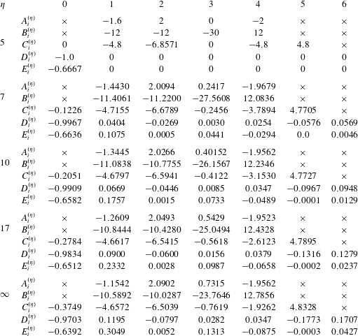
where the coefficients $D_{i}^{(\unicode[STIX]{x1D702})}$ and $E_{i}^{(\unicode[STIX]{x1D702})}$ are partially tabulated in table 3. Note that we have intentionally split the right-hand sides in (2.3) into two parts, so that the ‘generalized Grad 13-moment (GG13) equations’ can be extracted from (2.3) by setting

(2.5)$$\begin{eqnarray}m_{ijk}^{(\unicode[STIX]{x1D702})}=R_{ik}^{(\unicode[STIX]{x1D702})}=\unicode[STIX]{x1D6E5}^{(\unicode[STIX]{x1D702})}=\unicode[STIX]{x1D6F4}_{ij}^{(\unicode[STIX]{x1D702},2)}=Q_{i}^{(\unicode[STIX]{x1D702},2)}=0.\end{eqnarray}$$

The GG13 equations are introduced (Struchtrup Reference Struchtrup2005a) by the order of magnitude method, and its fully linearized version for hard spheres has been derived in Struchtrup & Torrilhon (Reference Struchtrup and Torrilhon2013).

Table 2.

Coefficients $C^{(\unicode[STIX]{x1D702})}$ for different $\unicode[STIX]{x1D702}$.

Table 3.

Coefficient of $A_{i}^{(\unicode[STIX]{x1D702})}$, $B_{i}^{(\unicode[STIX]{x1D702})}$, $C_{i}^{(\unicode[STIX]{x1D702})}$, $D_{i}^{(\unicode[STIX]{x1D702})}$ and $E_{i}^{(\unicode[STIX]{x1D702})}$ for different $\unicode[STIX]{x1D702}$.

To give the R13 equations, we need to close (2.3) by specifying $m_{ijk}^{(\unicode[STIX]{x1D702})}$, $R_{ik}^{(\unicode[STIX]{x1D702})}$, $\unicode[STIX]{x1D6E5}^{(\unicode[STIX]{x1D702})}$, $\unicode[STIX]{x1D6F4}_{ij}^{(\unicode[STIX]{x1D702},2)}$ and $Q_{i}^{(\unicode[STIX]{x1D702},2)}$. The closure depends on the specific form of the collision model. Here, we again assume that the collision is linearized about the local Maxwellian. Thus, the R13 theory gives the following closure:

(2.6)$$\begin{eqnarray}\left.\begin{array}{@{}c@{}}\displaystyle m_{ijk}^{(\unicode[STIX]{x1D702})}=\frac{\unicode[STIX]{x1D707}}{\unicode[STIX]{x1D703}\unicode[STIX]{x1D70C}}\left(A_{1}^{(\unicode[STIX]{x1D702})}q_{\langle \!i}{\displaystyle \frac{\unicode[STIX]{x2202}v_{j}}{\unicode[STIX]{x2202}x_{k\!\rangle }}}+A_{2}^{(\unicode[STIX]{x1D702})}\unicode[STIX]{x1D703}\unicode[STIX]{x1D70E}_{\langle \!ij}{\displaystyle \frac{\unicode[STIX]{x2202}\ln \unicode[STIX]{x1D70C}}{\unicode[STIX]{x2202}x_{k\!\rangle }}}+A_{3}^{(\unicode[STIX]{x1D702})}\unicode[STIX]{x1D70E}_{\langle \!ij}{\displaystyle \frac{\unicode[STIX]{x2202}\unicode[STIX]{x1D703}}{\unicode[STIX]{x2202}x_{k\!\rangle }}}+A_{4}^{(\unicode[STIX]{x1D702})}\unicode[STIX]{x1D703}{\displaystyle \frac{\unicode[STIX]{x2202}\unicode[STIX]{x1D70E}_{\langle \!ij}}{\unicode[STIX]{x2202}x_{k}\!\rangle }}\right),\\ \displaystyle \unicode[STIX]{x1D6E5}^{(\unicode[STIX]{x1D702})}=\frac{\unicode[STIX]{x1D707}}{\unicode[STIX]{x1D703}\unicode[STIX]{x1D70C}}\left(B_{1}^{(\unicode[STIX]{x1D702})}\unicode[STIX]{x1D703}{\displaystyle \frac{\unicode[STIX]{x2202}q_{k}}{\unicode[STIX]{x2202}x_{k}}}+B_{2}^{(\unicode[STIX]{x1D702})}\unicode[STIX]{x1D703}\unicode[STIX]{x1D70E}_{ij}{\displaystyle \frac{\unicode[STIX]{x2202}v_{i}}{\unicode[STIX]{x2202}x_{j}}}+B_{3}^{(\unicode[STIX]{x1D702})}q_{k}{\displaystyle \frac{\unicode[STIX]{x2202}\unicode[STIX]{x1D703}}{\unicode[STIX]{x2202}x_{k}}}+B_{4}^{(\unicode[STIX]{x1D702})}\unicode[STIX]{x1D703}q_{k}{\displaystyle \frac{\unicode[STIX]{x2202}\ln \unicode[STIX]{x1D70C}}{\unicode[STIX]{x2202}x_{k}}}\right),\\ \displaystyle \begin{array}{@{}rcl@{}}\displaystyle R_{ij}^{(\unicode[STIX]{x1D702})}\; & =\; & \displaystyle C_{0}^{(\unicode[STIX]{x1D702})}\unicode[STIX]{x1D703}\unicode[STIX]{x1D70E}_{ij}+\frac{\unicode[STIX]{x1D707}}{\unicode[STIX]{x1D703}\unicode[STIX]{x1D70C}}\left(C_{1}^{(\unicode[STIX]{x1D702})}\unicode[STIX]{x1D703}{\displaystyle \frac{\unicode[STIX]{x2202}q_{\langle \!i}}{\unicode[STIX]{x2202}x_{j\!\rangle }}}+C_{2}^{(\unicode[STIX]{x1D702})}\unicode[STIX]{x1D703}\unicode[STIX]{x1D70E}_{k\langle \!i}{\displaystyle \frac{\unicode[STIX]{x2202}v_{j\!\rangle }}{\unicode[STIX]{x2202}x_{k}}}+C_{3}^{(\unicode[STIX]{x1D702})}\unicode[STIX]{x1D703}^{2}\unicode[STIX]{x1D70C}{\displaystyle \frac{\unicode[STIX]{x2202}v_{\langle \!i}}{\unicode[STIX]{x2202}x_{j\!\rangle }}}\right.\\ \; & \; & \displaystyle +\left.C_{4}^{(\unicode[STIX]{x1D702})}q_{\langle \!i}{\displaystyle \frac{\unicode[STIX]{x2202}\unicode[STIX]{x1D703}}{\unicode[STIX]{x2202}x_{j\!\rangle }}}+C_{5}^{(\unicode[STIX]{x1D702})}\unicode[STIX]{x1D703}q_{\langle \!i}{\displaystyle \frac{\unicode[STIX]{x2202}\ln \unicode[STIX]{x1D70C}}{\unicode[STIX]{x2202}x_{j\!\rangle }}}\right).\end{array}\end{array}\right\}\end{eqnarray}$$

Some values of the coefficients $A_{i}^{(\unicode[STIX]{x1D702})}$, $B_{i}^{(\unicode[STIX]{x1D702})}$, and $C_{i}^{(\unicode[STIX]{x1D702})}$ are given in table 3. The full expressions of $\unicode[STIX]{x1D6F4}_{ij}^{(\unicode[STIX]{x1D702},2)}$ and $Q_{i}^{(\unicode[STIX]{x1D702},2)}$ are quite lengthy and we provide them in appendix C. A simple case is $\unicode[STIX]{x1D702}=5$, for which we have

(2.7a,b)$$\begin{eqnarray}\unicode[STIX]{x1D6F4}_{ij}^{(5,2)}=0,\quad Q_{i}^{(5,2)}=0,\end{eqnarray}$$

and the corresponding model matches that derived for Maxwell molecules by Struchtrup & Torrilhon (Reference Struchtrup and Torrilhon2003) (with terms nonlinear in $\unicode[STIX]{x1D70E}_{ij}$ and $q_{i}$ removed since we use the linearized collision model).

2.3 Discussion on the order of accuracy

One possible way to describe the accuracy of the moment models in the near-continuum regime is to use the notion of ‘order of accuracy’ (Struchtrup Reference Struchtrup2005a,Reference Struchtrupb). In such a regime, the Knudsen number $Kn$, i.e. the ratio of the mean free path to the characteristic length of the problem, is regarded as a small number. Thus, Chapman–Enskog expansion can be applied, and all non-equilibrium moments are expanded into power series of $Kn$, e.g.

(2.8)$$\begin{eqnarray}\left.\begin{array}{@{}c@{}}\unicode[STIX]{x1D70E}_{ij}=Kn\unicode[STIX]{x1D70E}_{ij}^{(1)}+Kn^{2}\unicode[STIX]{x1D70E}_{ij}^{(2)}+Kn^{3}\unicode[STIX]{x1D70E}_{ij}^{(3)}+\cdots \,,\\ q_{i}=Knq_{i}^{(1)}+Kn^{2}q_{i}^{(2)}+Kn^{3}q_{i}^{(3)}+\cdots \,.\end{array}\right\}\end{eqnarray}$$

By asymptotic analysis, all these terms can be represented by the conservative variables and their derivatives. Truncating the above series up to the term $Kn^{k}$ and inserting the result into (2.2), one obtains moment equations with $k$th order of accuracy. By this approach, the models derived from Chapman–Enskog expansion from zeroth to third order are, respectively, the Euler equations, the Navier–Stokes–Fourier equations, the Burnett equations and the super-Burnett equations. These equations contain only equilibrium variables: density, velocity and temperature.

In the 13-moment model, one can also assume $Kn$ is small and apply the expansion (2.8) to obtain models including only equilibrium variables. Suppose the second-order Chapman–Enskog expansion of a moment model agrees with the Burnett equations, while its third-order Chapman–Enskog expansion differs from super-Burnett equations, then we say that the moment model has the second-order accuracy (or Burnett order). For example, Grad’s 13-moment equations have the first-order accuracy for general IPL potentials, but have second-order accuracy for Maxwell molecules; GG13 equations are extensions to Grad’s 13-moment theory to achieve second-order accuracy for all molecule potentials. In general, the expansion (2.8) is usually obtained by multiplying the equations of $\unicode[STIX]{x1D70E}_{ij}$ and $q_{i}$ in the moment system by $Kn$. Therefore, in most cases, a 13-moment model has $k$th-order accuracy if the equations for $\unicode[STIX]{x1D70E}_{ij}$ and $q_{i}$ (2.3) are accurate up to the $(k-1)$th order. R13 equations have third-order accuracy, as the closure (2.6) provides the equations (2.3) exact second-order contributions.

In the literature, there exist similar 13-moment models obtained by other approaches to including second-order derivatives in the equations for $\unicode[STIX]{x1D70E}_{ij}$ and $q_{i}$. For instance, the relaxed Burnett equations (Jin & Slemrod Reference Jin and Slemrod2001) are also derived for arbitrary interaction potentials, and as mentioned in Jin & Slemrod (Reference Jin and Slemrod2001) and Struchtrup (Reference Struchtrup2005b), these equations have second-order accuracy. Another similar model is the nonlinear coupled constitutive relation equation model (Myong Reference Myong1999). These equations do not include information from the Burnett order, and therefore they have first-order accuracy and distinguish different interaction models by viscosity and heat conductivity coefficients. The full R13 models for Maxwell molecules and the Bhatnagar–Gross–Krook (BGK) model, which have third-order accuracy, have been derived in Struchtrup & Torrilhon (Reference Struchtrup and Torrilhon2003) and Struchtrup (Reference Struchtrup2005b), and the linear R13 equations for the hard-sphere model have been derived in Struchtrup & Torrilhon (Reference Struchtrup and Torrilhon2013).

2.4 Linear stability and dispersion

For the newly proposed R13 equations for IPL models, we are going to check some of its basic properties in this work. In this section, we focus on the linear properties, including stability in time and space, and the dispersion and damping of sound waves.

Following Struchtrup & Torrilhon (Reference Struchtrup and Torrilhon2003, Reference Struchtrup and Torrilhon2013) and Struchtrup (Reference Struchtrup2005b), we apply the analysis to one-dimensional linear dimensionless equations. The linearization is performed about a global equilibrium state with density $\unicode[STIX]{x1D70C}_{0}$, zero velocity and temperature $\unicode[STIX]{x1D703}_{0}$. The derivation of the one-dimensional linear dimensionless equations consists of the following steps.

1. (i) Introduce the small dimensionless variables $\hat{\unicode[STIX]{x1D70C}}$, $\hat{\unicode[STIX]{x1D703}}$, $\hat{v}_{i}$, $\hat{\unicode[STIX]{x1D70E}}_{ij}$ and $\hat{q}_{i}$ by

   (2.9a-e)$$\begin{eqnarray}\unicode[STIX]{x1D70C}=\unicode[STIX]{x1D70C}_{0}(1+\hat{\unicode[STIX]{x1D70C}}),\quad \unicode[STIX]{x1D703}=\unicode[STIX]{x1D703}_{0}(1+\hat{\unicode[STIX]{x1D703}}),\quad v_{i}=\sqrt{\unicode[STIX]{x1D703}_{0}}\hat{v}_{i},\quad \unicode[STIX]{x1D70E}_{ij}=\unicode[STIX]{x1D70C}_{0}\unicode[STIX]{x1D703}_{0}\hat{\unicode[STIX]{x1D70E}}_{ij},\quad q_{i}=\unicode[STIX]{x1D70C}_{0}\sqrt{\unicode[STIX]{x1D703}_{0}}^{3}\hat{q}_{i}.\end{eqnarray}$$

2. (ii) Let $L$ be the characteristic length, and define the dimensionless space and time variables by

   (2.10a,b)$$\begin{eqnarray}x_{i}=L\hat{x}_{i},\quad t=\frac{L}{\sqrt{\unicode[STIX]{x1D703}_{0}}}\hat{t}.\end{eqnarray}$$

3. (iii) Substitute (2.9) and (2.10) into the R13 equations (2.2), (2.3) and (2.6), and drop all the terms nonlinear in the variables with hats introduced in (2.9).

4. (iv) Reduce the resulting equations to a one-dimensional system by dropping all the terms with derivatives with respect to $x_{2}$ and $x_{3}$, and setting

   (2.11)$$\begin{eqnarray}\left.\begin{array}{@{}c@{}}\hat{v}_{1}=\hat{v},\quad \hat{q}_{1}=\hat{q},\quad \hat{\unicode[STIX]{x1D70E}}_{11}=\hat{\unicode[STIX]{x1D70E}},\quad \hat{\unicode[STIX]{x1D70E}}_{22}=\hat{\unicode[STIX]{x1D70E}}_{33}=-{\textstyle \frac{1}{2}}\hat{\unicode[STIX]{x1D70E}},\\ \hat{v}_{2}=\hat{v}_{3}=\hat{q}_{2}=\hat{q}_{3}=\hat{\unicode[STIX]{x1D70E}}_{12}=\hat{\unicode[STIX]{x1D70E}}_{23}=\hat{\unicode[STIX]{x1D70E}}_{13}=0.\end{array}\right\}\end{eqnarray}$$

The resulting equations can be written down more neatly if we introduce the Knudsen number

(2.12)$$\begin{eqnarray}Kn=\frac{\unicode[STIX]{x1D707}_{0}\sqrt{\unicode[STIX]{x1D703}_{0}}}{\unicode[STIX]{x1D70C}_{0}\unicode[STIX]{x1D703}_{0}L},\end{eqnarray}$$

where $\unicode[STIX]{x1D707}_{0}$ is the viscosity coefficient at temperature $\unicode[STIX]{x1D703}_{0}$. For all IPL models, the one-dimensional linear dimensionless equations have the form

(2.13)

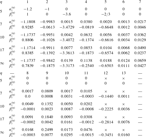
where $\unicode[STIX]{x1D6FC}_{i}^{(\unicode[STIX]{x1D702})}$ and $\unicode[STIX]{x1D6FD}_{i}^{(\unicode[STIX]{x1D702})}$ depend only on $\unicode[STIX]{x1D702}$, and their values for some choices of $\unicode[STIX]{x1D702}$ are listed in table 4. In (

), if we replace all the terms with double underlines by zero, we obtain the linearized GG13 equations. Furthermore, if we set all the terms with both single and double underlines to zero, then the result is the linearized Navier–Stokes–Fourier equations. The left-hand side of (

) comes from the advection, and the right-hand side comes from the collision. By table 4, it can be clearly seen that when $\unicode[STIX]{x1D702}=5$ (Maxwell molecules), due to the simplicity of the collision operator, all the underlined terms on the right-hand side disappear.

Table 4.

Coefficients of the linearized R13 system for different $\unicode[STIX]{x1D702}$.

For simplicity, we omit the hats on the variables hereafter. In general, the linear GG13 or R13 system has the form

(2.14)$$\begin{eqnarray}{\displaystyle \frac{\unicode[STIX]{x2202}u_{A}}{\unicode[STIX]{x2202}t}}+{\mathcal{A}}_{1}^{(\unicode[STIX]{x1D702})}{\displaystyle \frac{\unicode[STIX]{x2202}u_{A}}{\unicode[STIX]{x2202}x}}+{\mathcal{A}}_{2}^{(\unicode[STIX]{x1D702})}{\displaystyle \frac{\unicode[STIX]{x2202}^{2}u_{A}}{\unicode[STIX]{x2202}x^{2}}}+{\mathcal{A}}_{3}^{(\unicode[STIX]{x1D702})}u_{A}=0,\end{eqnarray}$$

where $u_{A}=(\unicode[STIX]{x1D70C},v,\unicode[STIX]{x1D703},\unicode[STIX]{x1D70E},q)^{\text{T}}$ and the matrices ${\mathcal{A}}_{i}^{(\unicode[STIX]{x1D702})}$ are constant matrices which can be observed from (2.13). To study the linear waves, we consider the plane wave solution

(2.15)$$\begin{eqnarray}u_{A}(x,t)=\tilde{u} _{A}\exp [\text{i}(\unicode[STIX]{x1D6FA}t-kx)],\end{eqnarray}$$

where $\tilde{u} _{A}$ is the initial amplitude of the wave, $\unicode[STIX]{x1D6FA}$ is frequency and $k$ is the wavenumber. Inserting the above solution into (2.14) yields

(2.16)$$\begin{eqnarray}{\mathcal{G}}^{(\unicode[STIX]{x1D702})}\tilde{u} _{A}=0,\quad \text{where }{\mathcal{G}}^{(\unicode[STIX]{x1D702})}=(\text{i}\unicode[STIX]{x1D6FA}-\text{i}k{\mathcal{A}}_{1}^{(\unicode[STIX]{x1D702})}-k^{2}{\mathcal{A}}_{2}^{(\unicode[STIX]{x1D702})}+{\mathcal{A}}_{3}^{(\unicode[STIX]{x1D702})}),\end{eqnarray}$$

and the existence of non-trivial solutions requires

(2.17)$$\begin{eqnarray}\det [{\mathcal{G}}^{(\unicode[STIX]{x1D702})}]=0.\end{eqnarray}$$

From (2.17), we can obtain the relation between $\unicode[STIX]{x1D6FA}$ and $k$, and thus all the desired properties such as the amplification and dispersion of the linear waves can naturally be obtained. In the following analysis, we choose $Kn=1$ to obtain quantitative results.

2.4.1 Linear stability in time and space

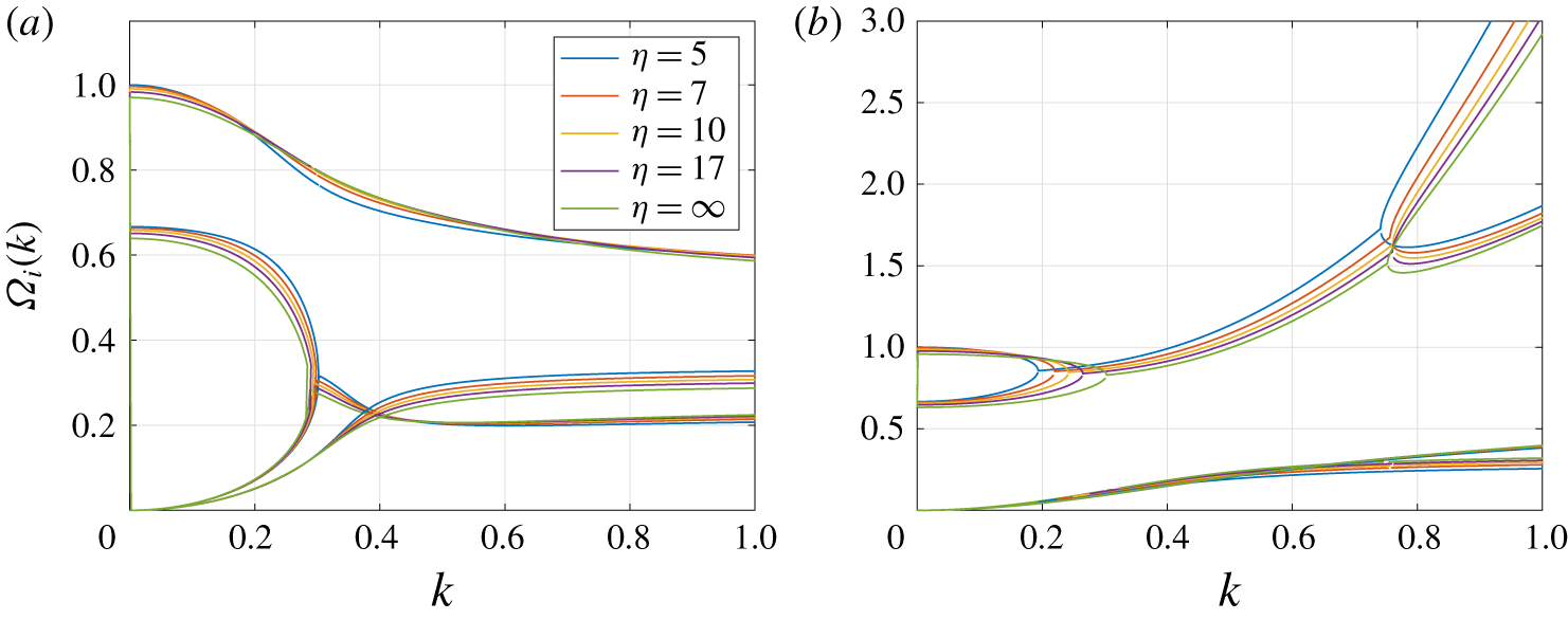
We first discuss the linear stability of the GG13 and R13 systems in time and space. For the time stability, we require that the norm of the amplitude decreases with time for any given wavenumber $k\in \mathbb{R}$. Precisely, if we assume $\unicode[STIX]{x1D6FA}=\unicode[STIX]{x1D6FA}_{r}(k)+\text{i}\unicode[STIX]{x1D6FA}_{i}(k)$, the time stability requires $\unicode[STIX]{x1D6FA}_{i}(k)\geqslant 0$. Figure 1 shows possible values of $\unicode[STIX]{x1D6FA}_{i}(k)$ on the complex plane. Note that $\unicode[STIX]{x1D6FA}_{i}(k)$ is a multi-valued function since (2.17) may have multiple solutions for a given $k$. It is observed that, for all choices $\unicode[STIX]{x1D702}$, the values of $\unicode[STIX]{x1D6FA}(k)$ are always located on the upper half of the complex plane, indicating linear stability for both R13 and GG13 equations.

Figure 1.

Damping coefficients $\unicode[STIX]{x1D6FA}_{i}(k)$ of the GG13 and R13 systems for different $\unicode[STIX]{x1D702}$.

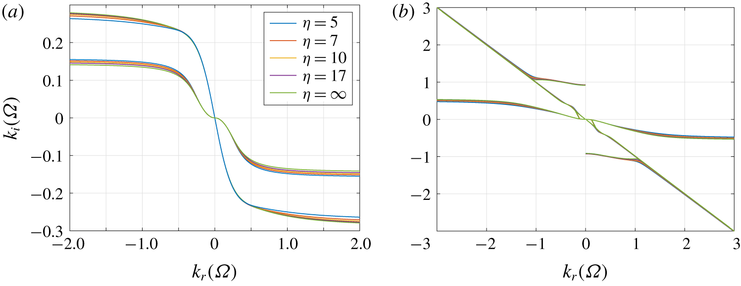
For the stability in space, we require that, for a given wave frequency, the amplitude should not increase along the direction of wave propagation. Now, we assume that $\unicode[STIX]{x1D6FA}\in \mathbb{R}$ is given, and let $k=k_{r}(\unicode[STIX]{x1D6FA})+\text{i}k_{i}(\unicode[STIX]{x1D6FA})$. Then the wave is stable in space if $k_{r}(\unicode[STIX]{x1D6FA})k_{i}(\unicode[STIX]{x1D6FA})\leqslant 0$. Figure 2 shows the values of $k$ in the complex plane with $\unicode[STIX]{x1D6FA}$ as the parameter. The results show that all the curves do not enter the upper right or the lower left quadrant for both the R13 and GG13 equations, showing the spatial stability for both models. Again, such a stability result holds for all $\unicode[STIX]{x1D702}$ considered in our experiments.

Figure 2.

The solutions $k(\unicode[STIX]{x1D6FA})$ of the dispersion relation in the complex plane with $\unicode[STIX]{x1D6FA}$ as the parameter of the GG13 and R13 systems for different $\unicode[STIX]{x1D702}$.

2.4.2 Dispersion and damping

We proceed by discussing the phase speeds as functions of frequency for the R13 and GG13 systems. For a given wave frequency $\unicode[STIX]{x1D6FA}$, we define the damping rate $\unicode[STIX]{x1D6FC}$ and the wave speed $v_{ph}$ by

(2.18a,b)$$\begin{eqnarray}\unicode[STIX]{x1D6FC}=-k_{i}(\unicode[STIX]{x1D6FA}),\quad v_{ph}=\frac{\unicode[STIX]{x1D6FA}}{k_{r}(\unicode[STIX]{x1D6FA})}.\end{eqnarray}$$

For the Euler equations, where $\unicode[STIX]{x1D70E}=q=0$ in (2.13), the absolute phase velocity is $|v_{ph}|=\sqrt{5/3}$ for all wave frequencies $\unicode[STIX]{x1D6FA}$. For R13 and GG13 equations, $v_{ph}$ depends on $\unicode[STIX]{x1D6FA}$, causing the dispersion of sound waves. Here, we define the dimensionless phase speed $c_{ph}=v_{ph}/\sqrt{5/3}$ and plot $c_{ph}$ as a function of the frequency $\unicode[STIX]{x1D6FA}$ in figure 3 for the R13 and GG13 equations. 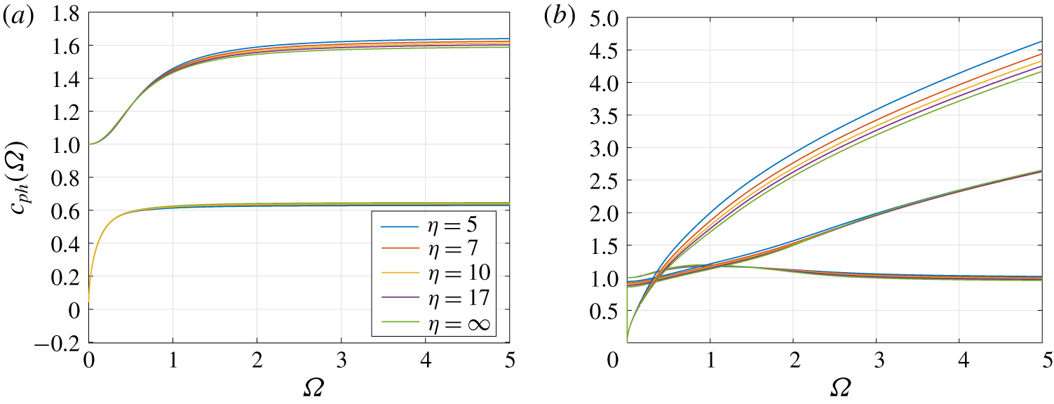Note that $c_{ph}(\unicode[STIX]{x1D6FA})$ is also a multi-valued function, and in figure 3, we only plot the positive phase velocities. For the GG13 equations, the phase velocity has an upper limit, indicating the hyperbolic nature of the system, while the R13 equations can achieve infinitely large phase velocities. In general, the phase speeds do not change much as $\unicode[STIX]{x1D702}$ varies, which predicts similar behaviour of sound waves in different monatomic gases.

Figure 3.

Phase speed $c_{ph}$ over frequency $\unicode[STIX]{x1D6FA}$ of the GG13 and R13 systems for different $\unicode[STIX]{x1D702}$.

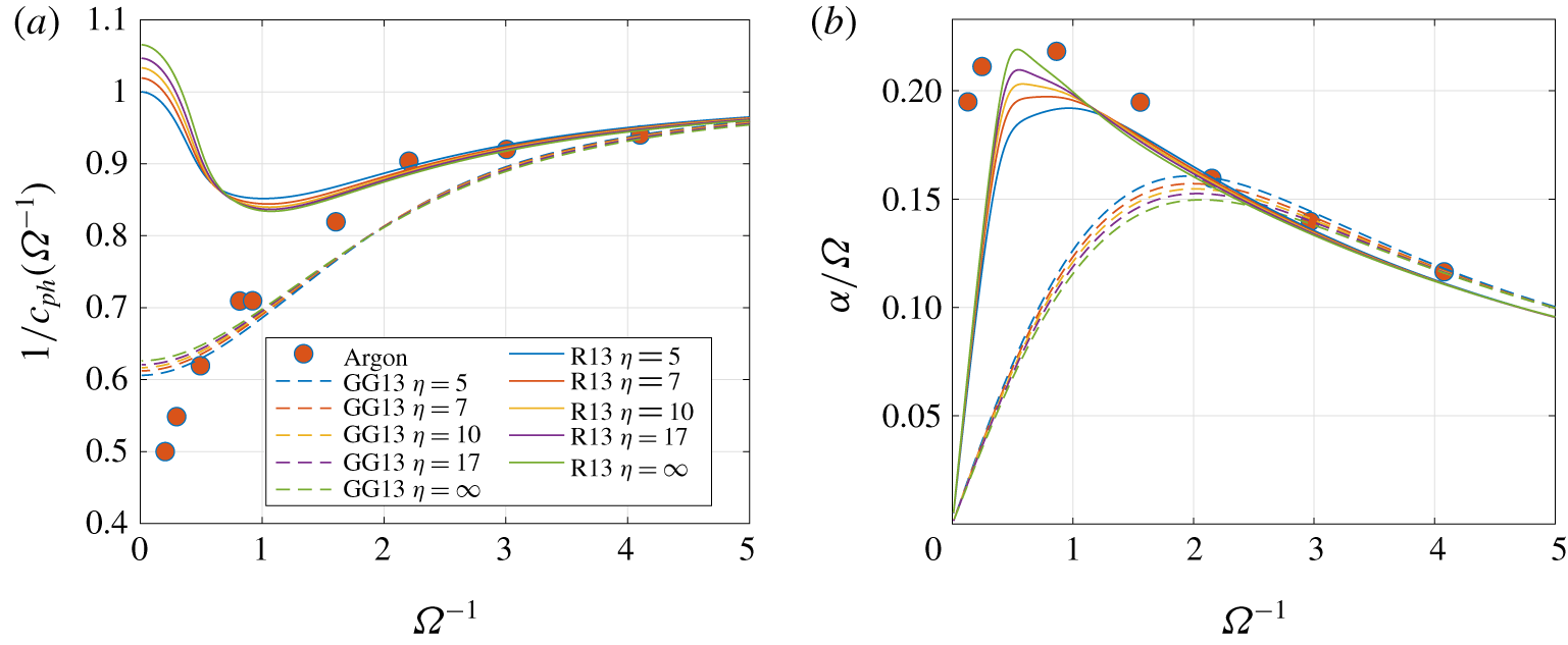
To study the phase speeds for large frequency waves, we plot the inverse wave speed $1/c_{ph}$ as a function of the inverse frequency $1/\unicode[STIX]{x1D6FA}$ in figure 4(a), and the reduced damping rate $\unicode[STIX]{x1D6FC}/\unicode[STIX]{x1D6FA}$ is plotted in figure 4(b) also as a function of $1/\unicode[STIX]{x1D6FA}$. In these figures, only the mode with the weakest damping is given. Figure 4(a) shows that, for the GG13 equations, the phase velocity increases monotonically as the frequency increases, while for the R13 equations, the wave slows down as $\unicode[STIX]{x1D6FA}$ reaches a value close to $1$. Such an observation agrees with the results in Struchtrup & Torrilhon (Reference Struchtrup and Torrilhon2003, Reference Struchtrup and Torrilhon2013), while the experimental results for argon (Meyer & Sessler Reference Meyer and Sessler1957) suggest the monotonicity of the phase velocity, which is closer to the prediction of the GG13 equations. Note that, here, we set the Knudsen number $Kn$ to be $1$. For another Knudsen number, the actual frequency of the wave should be $\unicode[STIX]{x1D6FA}/Kn$. This means that, if we consider a wave with a fixed actual frequency travelling in the gas with a low Knudsen number, we need to focus on large values of $\unicode[STIX]{x1D6FA}^{-1}$. Indeed, when $\unicode[STIX]{x1D6FA}^{-1}>1$, R13 models give a better approximation of the phase velocity, while for small $\unicode[STIX]{x1D6FA}^{-1}$, which corresponds to large Knudsen numbers, there is no guarantee as to whether the R13 or GG13 is superior, and the reason why GG13 provides better prediction requires further investigation. Nevertheless, for the damping rate shown in figure 4(b), R13 equations give significantly better agreement with the experimental data for the whole range of frequencies.

Figure 4.

Inverse phase speed and damping over frequency $\unicode[STIX]{x1D6FA}$ of the GG13 and R13 systems for different $\unicode[STIX]{x1D702}$. The bullets are the experimental results for argon Meyer & Sessler (Reference Meyer and Sessler1957).

3.1 General idea for the moment closure

Before providing the details of the derivation, we would first like to explain the general methodology of the moment closure. To close the advection term, one can observe from (2.3) that we need to provide expressions for the moments $m_{ijk}$, $R_{ik}$ and $\unicode[STIX]{x1D6E5}$, which correspond to the coefficients $f_{3m0}$, $f_{1m1}$ and $f_{002}$, respectively. To close the collision term, it can be seen from (3.4) that we have to provide expressions for infinite terms $f_{1mn}$ and $f_{2mn}$ for any positive integer $n$. In our implementation, this is done by a truncation of the infinite series in (3.4), whose fast convergence has already been demonstrated in Cai & Torrilhon (Reference Cai and Torrilhon2015), so that only a finite number of coefficients need to be considered.

The derivation of the R13 equations is similar to the Chapman–Enskog expansion. However, there are two key differences.

(K1)

All the moments are to be represented by the 13 moments and their derivatives, while only 5 equilibrium moments are involved in the Chapman–Enskog expansion.

(K2)

We expect that the equations have the Burnett order and involve only second-order derivatives, while third-order derivatives are involved in Burnett equations.

Due to the first difference, there are in principle infinite versions of the R13 equations in the Burnett order, since the leading-order terms in $\unicode[STIX]{x1D70E}_{ij}$ and $q_{i}$ can be represented by equilibrium variables

(3.6a,b)$$\begin{eqnarray}\unicode[STIX]{x1D70E}_{ij}\approx -\frac{2\unicode[STIX]{x1D707}}{\unicode[STIX]{x1D6FC}_{2}^{(\unicode[STIX]{x1D702})}}{\displaystyle \frac{\unicode[STIX]{x2202}v_{\langle \!i}}{\unicode[STIX]{x2202}x_{j\!\rangle }}},\quad q_{i}\approx -\frac{5\unicode[STIX]{x1D707}}{2\unicode[STIX]{x1D6FD}_{5}^{(\unicode[STIX]{x1D702})}}{\displaystyle \frac{\unicode[STIX]{x2202}\unicode[STIX]{x1D703}}{\unicode[STIX]{x2202}x_{i}}},\end{eqnarray}$$

as already derived in many different versions of R13 equations for Maxwell molecules (Timokhin et al. Reference Timokhin, Struchtrup, Kokhanchik and Bondar2017). In our derivation, since $\unicode[STIX]{x1D70E}_{ij}$ and $q_{i}$ are already included in the system, we will avoid using (3.6) to make any replacement except in the derivation of the first-order expressions. More precisely, according to the Chapman–Enskog expansion, the first-order term of the distribution function can be completely represented by the following quantities:

$$\begin{eqnarray}\unicode[STIX]{x1D70C},v_{i},\unicode[STIX]{x1D703},{\displaystyle \frac{\unicode[STIX]{x2202}v_{\langle \!i}}{\unicode[STIX]{x2202}x_{j\!\rangle }}},\quad {\displaystyle \frac{\unicode[STIX]{x2202}\unicode[STIX]{x1D703}}{\unicode[STIX]{x2202}x_{i}}}.\end{eqnarray}$$

At this step, we apply (3.6) to replace the derivatives of $v_{i}$ and $\unicode[STIX]{x1D703}$ by $\unicode[STIX]{x1D70E}_{ij}$ and $q_{i}$. By such replacement, one order of derivative can be eliminated, so that (K2) can be automatically achieved.

3.2 Chapman–Enskog expansion of the coefficients

This section is devoted to the details of the asymptotic analysis. As mentioned in the previous section, the idea of a Chapman–Enskog expansion is utilized here to derive models with different orders of accuracy. To begin with, we introduce the scaling $t=t^{\prime }/\unicode[STIX]{x1D716}$ and $x_{i}=x_{i}^{\prime }/\unicode[STIX]{x1D716}$, and rewrite equations (3.4) with time and spatial variables $t^{\prime }$ and $x_{i}^{\prime }$. In the resulting equations, a factor $\unicode[STIX]{x1D716}^{-1}$ is introduced to the right-hand side of (3.4). In this section, we work on the scaled equations, and the prime symbol on $t^{\prime }$ and $x_{i}^{\prime }$ is omitted. Based on such a transform, we write down the asymptotic expansion for all the moments as

(3.7)$$\begin{eqnarray}f_{lmn}=f_{lmn}^{(0)}+\unicode[STIX]{x1D716}f_{lmn}^{(1)}+\unicode[STIX]{x1D716}^{2}f_{lmn}^{(2)}+\unicode[STIX]{x1D716}^{3}f_{lmn}^{(3)}+\cdots \,.\end{eqnarray}$$

In the original Chapman–Enskog expansion of the distribution function $f=f^{(0)}+\unicode[STIX]{x1D716}f^{(1)}$, we require that $f^{(0)}$ is the local Maxwellian ${\mathcal{M}}$. The corresponding assumption for the coefficients is

(3.8)$$\begin{eqnarray}f_{lmn}^{(0)}=\left\{\begin{array}{@{}ll@{}}\unicode[STIX]{x1D70C}, & \text{if }(l,m,n)=(0,0,0),\\ 0, & \text{otherwise}.\end{array}\right.\end{eqnarray}$$

By (3.7), the terms $S_{lmn}$ and $T_{lmn}$ can be expanded correspondingly

(3.9a,b)$$\begin{eqnarray}S_{lmn}=S_{lmn}^{(0)}+\unicode[STIX]{x1D716}S_{lmn}^{(1)}+\unicode[STIX]{x1D716}^{2}S_{lmn}^{(2)}+\unicode[STIX]{x1D716}^{3}S_{lmn}^{(3)}+\cdots \,,\quad T_{lmn}=T_{lmn}^{(0)}+\unicode[STIX]{x1D716}T_{lmn}^{(1)}+\unicode[STIX]{x1D716}^{2}T_{lmn}^{(2)}+\unicode[STIX]{x1D716}^{3}T_{lmn}^{(3)}+\cdots \,.\end{eqnarray}$$

Note that the above expansion is straightforward since both $S_{lmn}$ and $T_{lmn}$ are linear in all the coefficients $f_{lmn}$. Thus, the moment equations turn out to be

(3.10)$$\begin{eqnarray}\displaystyle & & \displaystyle {\displaystyle \frac{\unicode[STIX]{x2202}(f_{lmn}^{(0)}+\unicode[STIX]{x1D716}f_{lmn}^{(1)}+\unicode[STIX]{x1D716}^{2}f_{lmn}^{(2)}+\unicode[STIX]{x1D716}^{3}f_{lmn}^{(3)}+\cdots \,)}{\unicode[STIX]{x2202}t}}\nonumber\\ \displaystyle & & \displaystyle \qquad +\,(S_{lmn}^{(0)}+\unicode[STIX]{x1D716}S_{lmn}^{(1)}+\unicode[STIX]{x1D716}^{2}S_{lmn}^{(2)}+\unicode[STIX]{x1D716}^{3}S_{lmn}^{(3)}+\cdots \,)+(T_{lmn}^{(0)}+\unicode[STIX]{x1D716}T_{lmn}^{(1)}+\unicode[STIX]{x1D716}^{2}T_{lmn}^{(2)}+\unicode[STIX]{x1D716}^{3}T_{lmn}^{(3)}+\cdots \,)\nonumber\\ \displaystyle & & \displaystyle \quad =\frac{1}{\unicode[STIX]{x1D716}}\left(\frac{\unicode[STIX]{x1D70C}\unicode[STIX]{x1D703}}{\unicode[STIX]{x1D707}}\mathop{\sum }_{n^{\prime }=0}^{+\infty }a_{lnn^{\prime }}\unicode[STIX]{x1D703}^{n-n^{\prime }}(f_{lmn^{\prime }}^{(0)}+\unicode[STIX]{x1D716}f_{lmn^{\prime }}^{(1)}+\unicode[STIX]{x1D716}^{2}f_{lmn^{\prime }}^{(2)}+\unicode[STIX]{x1D716}^{3}f_{lmn^{\prime }}^{(3)}+\cdots \,)\right).\end{eqnarray}$$

Matching the terms with the same orders with respect to $\unicode[STIX]{x1D716}$, one obtains

(3.11)$$\begin{eqnarray}{\displaystyle \frac{\unicode[STIX]{x2202}f_{lmn}^{(k)}}{\unicode[STIX]{x2202}t}}+S_{lmn}^{(k)}+T_{lmn}^{(k)}=\frac{\unicode[STIX]{x1D70C}\unicode[STIX]{x1D703}}{\unicode[STIX]{x1D707}}\mathop{\sum }_{n^{\prime }=0}^{+\infty }a_{lnn^{\prime }}\unicode[STIX]{x1D703}^{n-n^{\prime }}f_{lmn^{\prime }}^{(k+1)},\quad k\geqslant 0.\end{eqnarray}$$

In Chapman–Enskog expansion, due to the assumption (3.8), equation (3.11) is only applied to the case $(l,n)\neq (0,0),(1,0),(0,1)$, in which the right-hand side of (3.11) is non-zero and (3.11) can provide us expressions for $f_{lmn}^{(k+1)}$. For more details about the Chapman–Enskog expansion, we refer the reader to textbooks such as Struchtrup (Reference Struchtrup2005a). In what follows, we introduce a generalized version of the Chapman–Enskog expansion involving 13 moments in the assumption, which is carried out by studying each $k$ incrementally. Note that the idea of the following method is also applicable for more general collision models.

3.2.1 First order ($k=0$)

When $(l,n)\neq (0,0),(1,0),(0,1)$, using (3.8) and the fact that $S_{lmn}$ is a linear combination of (3.5), one can see that $f_{lmn}^{(0)}=S_{lmn}^{(0)}=0$. Thus, when $k=0$, equation (3.11) becomes

(3.12)$$\begin{eqnarray}T_{lmn}^{(0)}=\frac{\unicode[STIX]{x1D70C}\unicode[STIX]{x1D703}}{\unicode[STIX]{x1D707}}\mathop{\sum }_{n^{\prime }=0}^{+\infty }a_{lnn^{\prime }}\unicode[STIX]{x1D703}^{n-n^{\prime }}f_{lmn^{\prime }}^{(1)}.\end{eqnarray}$$

If $l=0$, $n>1$ or $l\geqslant 3$, the property (P2) and (3.8) show that $T_{lmn}^{(0)}=0$, meaning that

(3.13)$$\begin{eqnarray}f_{lmn}^{(1)}=0,\quad \text{if }l\geqslant 3\text{ or }l=0.\end{eqnarray}$$

In the following, we focus on the cases $l=1$ and $l=2$. Note that $f_{1m0}=0$, by which we can rewrite (3.12) as

(3.14a,b)$$\begin{eqnarray}T_{1mn}^{(0)}=\frac{\unicode[STIX]{x1D70C}\unicode[STIX]{x1D703}}{\unicode[STIX]{x1D707}}\mathop{\sum }_{n^{\prime }=1}^{+\infty }a_{1nn^{\prime }}\unicode[STIX]{x1D703}^{n-n^{\prime }}f_{1mn^{\prime }}^{(1)},\quad T_{2mn}^{(0)}=\frac{\unicode[STIX]{x1D70C}\unicode[STIX]{x1D703}}{\unicode[STIX]{x1D707}}\mathop{\sum }_{n^{\prime }=0}^{+\infty }a_{2nn^{\prime }}\unicode[STIX]{x1D703}^{n-n^{\prime }}f_{2mn^{\prime }}^{(1)}.\end{eqnarray}$$

Again by the property (P2) and (3.8), we see that $T_{1mn}^{(0)}=0$ for all $n>1$ and $T_{2mn}^{(0)}=0$ for all $n>0$. For any given $m$, the values of $f_{1mn^{\prime }}^{(1)}$ and $f_{2mn^{\prime }}^{(1)}$ can be solved from (3.14), and the result has the form

(3.15a,b)$$\begin{eqnarray}f_{1mn}^{(1)}=\frac{\unicode[STIX]{x1D707}}{\unicode[STIX]{x1D70C}\unicode[STIX]{x1D703}}A_{1n}\unicode[STIX]{x1D703}^{n-1}T_{1m1}^{(0)},\quad f_{2mn}^{(1)}=\frac{\unicode[STIX]{x1D707}}{\unicode[STIX]{x1D70C}\unicode[STIX]{x1D703}}A_{2n}\unicode[STIX]{x1D703}^{n}T_{2m0}^{(0)},\end{eqnarray}$$

where $A_{1n}$ and $A_{2n}$ are pure numbers. In principle, obtaining (3.15) requires solving an infinite matrix. In our implementation, this is approximated by a cutoff of the right-hand sides of (3.14) up to $n^{\prime }\leqslant 9$.

Until now, our calculation is completely the same as the classical Chapman–Enskog expansion. In (3.15), all first-order quantities can be represented by the conservative quantities and their derivatives (hidden in the expressions for $T_{1m1}^{(0)}$ and $T_{2m0}^{(0)}$). However, to derive 13-moment equations, we are required to represent the distribution functions using more moments and less derivatives. For example, in Grad’s 13-moment theory, no derivatives are included in the ansatz of the distribution function. In our derivation, this can be achieved by writing (3.15) as

(3.16a,b)$$\begin{eqnarray}f_{1mn}^{(1)}=\frac{A_{1n}}{A_{11}}\unicode[STIX]{x1D703}^{n-1}f_{1m1}^{(1)},\quad f_{2mn}^{(1)}=\frac{A_{2n}}{A_{20}}\unicode[STIX]{x1D703}^{n}f_{2m0}^{(1)}.\end{eqnarray}$$

Since $f_{2m0}$ and $f_{1m1}$ are included in the 13-moment theory, we mimic the assumption of Chapman–Enskog expansion (3.8) and set

(3.17a-c)$$\begin{eqnarray}f_{1m1}=\unicode[STIX]{x1D716}f_{1m1}^{(1)},\quad f_{2m0}=\unicode[STIX]{x1D716}f_{2m0}^{(1)},\quad f_{1m1}^{(k)}=f_{2m0}^{(k)}=0,\quad k\geqslant 2.\end{eqnarray}$$

By (3.16) and (3.17), we can write down the approximation of the distribution function up to first order in $\unicode[STIX]{x1D716}$ using the 13 moments

(3.18)$$\begin{eqnarray}\displaystyle f(\boldsymbol{x},\unicode[STIX]{x1D743},t) & {\approx} & \displaystyle {\mathcal{M}}(\boldsymbol{x},\unicode[STIX]{x1D743},t)+\mathop{\sum }_{m=-1}^{1}f_{1m1}(\boldsymbol{x},t)\mathop{\sum }_{n=1}^{+\infty }\frac{A_{1n}}{A_{11}}[\unicode[STIX]{x1D703}(\boldsymbol{x},t)]^{n-1}\unicode[STIX]{x1D713}_{1mn}(\boldsymbol{x},\unicode[STIX]{x1D743},t)\nonumber\\ \displaystyle & & \displaystyle +\,\mathop{\sum }_{m=-2}^{2}f_{2m0}(\boldsymbol{x},t)\mathop{\sum }_{n=0}^{+\infty }\frac{A_{2n}}{A_{20}}[\unicode[STIX]{x1D703}(\boldsymbol{x},t)]^{n}\unicode[STIX]{x1D713}_{2mn}(\boldsymbol{x},\unicode[STIX]{x1D743},t),\end{eqnarray}$$

where we have written all the parameters $t,\boldsymbol{x}$ and $\unicode[STIX]{x1D743}$ for clarification. Note that, in contrast to the Chapman–Enskog expansion of the distribution function, no derivatives are involved in the above expression. Equation (3.18) is also different from Grad’s ansatz for the 13-moment theory, since (3.18) can be written equivalently as

(3.19)$$\begin{eqnarray}\displaystyle & & \displaystyle f(\unicode[STIX]{x1D743})\approx \left[1-\mathop{\sum }_{i=1}^{3}\frac{(\unicode[STIX]{x1D709}_{i}-v_{i})q_{i}}{\unicode[STIX]{x1D703}^{2}}\mathop{\sum }_{n=1}^{+\infty }\frac{A_{1n}}{A_{11}}\sqrt{\frac{3\unicode[STIX]{x03C0}^{1/2}n!}{10\unicode[STIX]{x1D6E4}(n+5/2)}}L_{n}^{(3/2)}\left(\frac{\unicode[STIX]{x1D743}-\boldsymbol{v}}{2\unicode[STIX]{x1D703}}\right)\right.\nonumber\\ \displaystyle & & \displaystyle \quad +\left.\mathop{\sum }_{i=1}^{3}\mathop{\sum }_{j=1}^{3}\frac{\unicode[STIX]{x1D70E}_{ij}(\unicode[STIX]{x1D709}_{i}-v_{i})(\unicode[STIX]{x1D709}_{j}-v_{j})}{\unicode[STIX]{x1D703}^{2}}\mathop{\sum }_{n=0}^{+\infty }\frac{A_{2n}}{A_{20}}\sqrt{\frac{15\unicode[STIX]{x03C0}^{1/2}n!}{32\unicode[STIX]{x1D6E4}(n+7/2)}}L_{n}^{(5/2)}\left(\frac{\unicode[STIX]{x1D743}-\boldsymbol{v}}{2\unicode[STIX]{x1D703}}\right)\right]{\mathcal{M}}(\unicode[STIX]{x1D743}).\nonumber\\ \displaystyle & & \displaystyle\end{eqnarray}$$

Here, $L_{n}^{(\unicode[STIX]{x1D6FC})}$ is the Laguerre polynomial defined in (B 2), and we have omitted the variables $t$ and $\boldsymbol{x}$ for conciseness. Grad’s ansatz for the 13-moment theory can be obtained by truncating both infinite sums in (3.19) by preserving only their first terms, and therefore Grad’s 13-moment theory does not fully represent the first-order term of the distribution function for general collision models. Due to the assumption (3.17), when we apply (3.11), equations for all the 13 moments should be excluded, i.e. $(l,n)\neq (0,0),(0,1),(1,0),(1,1),(2,0)$.

Remark 3. The solvability of (3.14) relies on the existence of the spectral gap for the linearized Boltzmann collision operator. For IPL models, this has been proven in Mouhot & Strain (Reference Mouhot and Strain2007). In particular, when $\unicode[STIX]{x1D702}=5$, we have $A_{1n}=\unicode[STIX]{x1D6FF}_{1n}/a_{111}$ and $A_{2n}=\unicode[STIX]{x1D6FF}_{0n}/a_{200}$. In this case, the first two orders (3.18) are exactly the ansatz in Grad’s 13-moment theory.

3.2.2 Second order ($k=1$)

Now we set $k=1$ in (3.11). Since $f_{000}=f_{001}=f_{1m0}=0$ and $f_{2m0}^{(k)}=f_{1m1}^{(k)}=0$ for $k\geqslant 2$, the result can be written as

(3.20)$$\begin{eqnarray}{\displaystyle \frac{\unicode[STIX]{x2202}f_{lmn}^{(1)}}{\unicode[STIX]{x2202}t}}+S_{lmn}^{(1)}+T_{lmn}^{(1)}=\frac{\unicode[STIX]{x1D70C}\unicode[STIX]{x1D703}}{\unicode[STIX]{x1D707}}\mathop{\sum }_{n^{\prime }=n_{0}(l)}^{+\infty }a_{lnn^{\prime }}\unicode[STIX]{x1D703}^{n-n^{\prime }}f_{lmn^{\prime }}^{(2)},\end{eqnarray}$$

where

(3.21)$$\begin{eqnarray}n_{0}(l)=\left\{\begin{array}{@{}ll@{}}2, & \text{if }l=0,1,\\ 1, & \text{if }l=2,\\ 0, & \text{if }l\geqslant 3.\end{array}\right.\end{eqnarray}$$

Since $f_{lmn}^{(1)}$ has been fully obtained in the previous section (see (3.13) and (3.17)), the expressions of $S_{lmn}^{(1)}$ and $T_{lmn}^{(1)}$ can be naturally obtained. Thus, the left-hand side of (3.20) can already be represented by the 13 moments. To obtain the second-order contributions $f_{lmn}^{(2)}$, for any $l$ and $m$, we just need to solve the infinite linear system (3.20), and the general result is

(3.22)$$\begin{eqnarray}f_{lmn}^{(2)}=\frac{\unicode[STIX]{x1D707}}{\unicode[STIX]{x1D70C}\unicode[STIX]{x1D703}}\mathop{\sum }_{n^{\prime }=n_{0}(l)}^{+\infty }B_{lnn^{\prime }}\unicode[STIX]{x1D703}^{n-n^{\prime }}\left({\displaystyle \frac{\unicode[STIX]{x2202}f_{lmn^{\prime }}^{(1)}}{\unicode[STIX]{x2202}t}}+S_{lmn^{\prime }}^{(1)}+T_{lmn^{\prime }}^{(1)}\right),\end{eqnarray}$$

where $B_{lnn^{\prime }}$ are all pure numbers. In our implementation, we again truncate the system (3.20) at $n^{\prime }=\lfloor 10-l/2\rfloor$. For the purpose of deriving R13 equations, we only need $f_{lmn}^{(2)}$ up to $l=4$.

The right-hand side of (3.22) still contains time derivatives, which are not desired. In general, they can all be replaced by spatial derivatives. Note that $\unicode[STIX]{x2202}_{t}\,f_{lmn}^{(1)}$ is non-zero only if $l=1$ or $l=2$. In these cases, we have

(3.23)$$\begin{eqnarray}\left.\begin{array}{@{}c@{}}\displaystyle \frac{\unicode[STIX]{x2202}f_{1mn^{\prime }}^{(1)}}{\unicode[STIX]{x2202}t}=\frac{A_{1n^{\prime }}}{A_{11}}\left(\unicode[STIX]{x1D703}^{n^{\prime }-1}\frac{\unicode[STIX]{x2202}f_{1m1}^{(1)}}{\unicode[STIX]{x2202}t}+(n^{\prime }-1)\unicode[STIX]{x1D703}^{n^{\prime }-2}{\displaystyle \frac{\unicode[STIX]{x2202}\unicode[STIX]{x1D703}}{\unicode[STIX]{x2202}t}}f_{1m1}^{(1)}\right),\\ \displaystyle \frac{\unicode[STIX]{x2202}f_{2mn^{\prime }}^{(1)}}{\unicode[STIX]{x2202}t}=\frac{A_{2n^{\prime }}}{A_{20}}\left(\unicode[STIX]{x1D703}^{n^{\prime }}\frac{\unicode[STIX]{x2202}f_{2m0}^{(1)}}{\unicode[STIX]{x2202}t}+n^{\prime }\unicode[STIX]{x1D703}^{n^{\prime }-1}{\displaystyle \frac{\unicode[STIX]{x2202}\unicode[STIX]{x1D703}}{\unicode[STIX]{x2202}t}}f_{2m0}^{(1)}\right).\end{array}\right\}\end{eqnarray}$$

We first focus on $\unicode[STIX]{x2202}_{t}\,f_{1m1}^{(1)}$ and $\unicode[STIX]{x2202}_{t}\,f_{2m0}^{(1)}$. Taking $\unicode[STIX]{x2202}_{t}\,f_{1m1}^{(1)}$ as an example, we perform the following calculation:

(3.24)

from which it can be solved that

(3.25)$$\begin{eqnarray}\displaystyle \frac{\unicode[STIX]{x2202}f_{1m1}^{(1)}}{\unicode[STIX]{x2202}t} & = & \displaystyle \left(1-\mathop{\sum }_{n^{\prime }=2}^{+\infty }\unicode[STIX]{x1D706}_{1n^{\prime }}\right)^{-1}\left[\frac{1}{\unicode[STIX]{x1D716}}\left(\frac{\unicode[STIX]{x1D70C}\unicode[STIX]{x1D703}}{\unicode[STIX]{x1D707}}\frac{f_{1m1}^{(1)}}{A_{11}}-T_{1m1}^{(0)}\right)\right.\nonumber\\ \displaystyle & & \displaystyle +\left.\mathop{\sum }_{n^{\prime }=2}^{+\infty }\frac{(n^{\prime }-1)\unicode[STIX]{x1D706}_{1n^{\prime }}}{\unicode[STIX]{x1D703}}{\displaystyle \frac{\unicode[STIX]{x2202}\unicode[STIX]{x1D703}}{\unicode[STIX]{x2202}t}}f_{1m1}^{(1)}+\mathop{\sum }_{n^{\prime }=1}^{+\infty }C_{1n^{\prime }}\unicode[STIX]{x1D703}^{1-n^{\prime }}(S_{1mn^{\prime }}^{(1)}+T_{1mn^{\prime }}^{(1)})\right]+O(\unicode[STIX]{x1D716}),\qquad\end{eqnarray}$$

where we have used $S_{1m1}^{(0)}=0$, and the newly introduced constants are

(3.26a,b)$$\begin{eqnarray}C_{ln^{\prime }}=\left\{\begin{array}{@{}ll@{}}-1, & \text{if }n^{\prime }=n_{0}(l)-1,\\ \displaystyle \mathop{\sum }_{n=n_{0}(l)}^{+\infty }a_{l,n_{0}(l)-1,n}B_{lnn^{\prime }}, & \text{if }n^{\prime }\geqslant n_{0}(l),\end{array}\right.\quad \unicode[STIX]{x1D706}_{ln^{\prime }}=\frac{C_{ln^{\prime }}A_{ln^{\prime }}}{A_{l,n_{0}(l)-1}}.\end{eqnarray}$$

Similarly, we can obtain

(3.27)$$\begin{eqnarray}\displaystyle \frac{\unicode[STIX]{x2202}f_{2m0}^{(1)}}{\unicode[STIX]{x2202}t} & = & \displaystyle \left(1-\mathop{\sum }_{n^{\prime }=1}^{+\infty }\unicode[STIX]{x1D706}_{2n^{\prime }}\right)^{-1}\left[\frac{1}{\unicode[STIX]{x1D716}}\left(\frac{\unicode[STIX]{x1D70C}\unicode[STIX]{x1D703}}{\unicode[STIX]{x1D707}}\frac{f_{2m0}^{(1)}}{A_{20}}-T_{2m0}^{(0)}\right)\right.\nonumber\\ \displaystyle & & \displaystyle +\left.\mathop{\sum }_{n^{\prime }=1}^{+\infty }\frac{n^{\prime }\unicode[STIX]{x1D706}_{2n^{\prime }}}{\unicode[STIX]{x1D703}}{\displaystyle \frac{\unicode[STIX]{x2202}\unicode[STIX]{x1D703}}{\unicode[STIX]{x2202}t}}f_{2m0}^{(1)}+\mathop{\sum }_{n^{\prime }=0}^{+\infty }C_{2n^{\prime }}\unicode[STIX]{x1D703}^{-n^{\prime }}(S_{2mn^{\prime }}^{(1)}+T_{2mn^{\prime }}^{(1)})\right]+O(\unicode[STIX]{x1D716}).\end{eqnarray}$$

As a summary, the time derivatives in (3.22) can be replaced with spatial derivatives by the following operations.

1. (i) If $l\neq 1$ and $l\neq 2$, set the derivative $\unicode[STIX]{x2202}_{t}\,f_{lmn^{\prime }}^{(1)}$ to zero. If $l=1$ or $l=2$, replace $\unicode[STIX]{x2202}_{t}\,f_{1mn^{\prime }}^{(1)}$ by (3.23), (3.25) and (3.27).

2. (ii) After replacement, the results still include the time derivatives of $\boldsymbol{v}$ and $\unicode[STIX]{x1D703}$. These terms can be replaced by conservation laws (2.2). In fact, we can use the fact that $\unicode[STIX]{x1D70E}_{kl}$ and $q_{k}$ are $O(\unicode[STIX]{x1D716})$ terms to rewrite the conservation laws of momentum and energy as

   (3.28a,b)$$\begin{eqnarray}\frac{\unicode[STIX]{x2202}v_{i}}{\unicode[STIX]{x2202}t}=-v_{k}{\displaystyle \frac{\unicode[STIX]{x2202}v_{i}}{\unicode[STIX]{x2202}x_{k}}}-\frac{\unicode[STIX]{x1D703}}{\unicode[STIX]{x1D70C}}{\displaystyle \frac{\unicode[STIX]{x2202}\unicode[STIX]{x1D70C}}{\unicode[STIX]{x2202}x_{i}}}-{\displaystyle \frac{\unicode[STIX]{x2202}\unicode[STIX]{x1D703}}{\unicode[STIX]{x2202}x_{i}}}+O(\unicode[STIX]{x1D716}),\quad \frac{\unicode[STIX]{x2202}\unicode[STIX]{x1D703}}{\unicode[STIX]{x2202}t}=-\frac{2}{3}\unicode[STIX]{x1D703}{\displaystyle \frac{\unicode[STIX]{x2202}v_{k}}{\unicode[STIX]{x2202}x_{k}}}-v_{k}{\displaystyle \frac{\unicode[STIX]{x2202}\unicode[STIX]{x1D703}}{\unicode[STIX]{x2202}x_{k}}}+O(\unicode[STIX]{x1D716}),\end{eqnarray}$$
   and use these equations for substitution.

3. (iii) After the above replacements, the $O(\unicode[STIX]{x1D716})$ terms can be dropped.

By now, we have presented all the coefficients $f_{lmn}^{(2)}$ by the 13 moments and their spatial derivatives. When $l=1,2$, the results include a coefficient $1/\unicode[STIX]{x1D716}$ coming from (3.25) and (3.27). More precisely, $f_{1mn}^{(2)}$ and $f_{2mn}^{(2)}$ have the form

(3.29)$$\begin{eqnarray}\displaystyle & \displaystyle f_{1mn}^{(2)}=\frac{1}{\unicode[STIX]{x1D716}}\unicode[STIX]{x1D703}^{n-1}\left(\mathop{\sum }_{n^{\prime }=2}^{+\infty }B_{1nn^{\prime }}\frac{A_{1n^{\prime }}}{A_{11}}\right)\left(1-\mathop{\sum }_{n^{\prime }=2}^{+\infty }\unicode[STIX]{x1D706}_{1n^{\prime }}\right)^{-1}\left(\frac{f_{1m1}^{(1)}}{A_{11}}-\frac{\unicode[STIX]{x1D707}}{\unicode[STIX]{x1D70C}\unicode[STIX]{x1D703}}T_{1m1}^{(0)}\right)+W_{1mn}^{(2)},\quad n\geqslant 2, & \displaystyle \nonumber\\ \displaystyle & & \displaystyle\end{eqnarray}$$

(3.30)$$\begin{eqnarray}\displaystyle & \displaystyle f_{2mn}^{(2)}=\frac{1}{\unicode[STIX]{x1D716}}\unicode[STIX]{x1D703}^{n}\left(\mathop{\sum }_{n^{\prime }=1}^{+\infty }B_{2nn^{\prime }}\frac{A_{2n^{\prime }}}{A_{20}}\right)\left(1-\mathop{\sum }_{n^{\prime }=1}^{+\infty }\unicode[STIX]{x1D706}_{2n^{\prime }}\right)^{-1}\left(\frac{f_{2m0}^{(1)}}{A_{20}}-\frac{\unicode[STIX]{x1D707}}{\unicode[STIX]{x1D70C}\unicode[STIX]{x1D703}}T_{2m0}^{(0)}\right)+W_{2mn}^{(2)},\quad n\geqslant 1, & \displaystyle \nonumber\\ \displaystyle & & \displaystyle\end{eqnarray}$$

where $W_{1mn}^{(2)}$ and $W_{2mn}^{(2)}$ are terms independent of $\unicode[STIX]{x1D716}$. Note that only first-order derivatives have been introduced into $f_{lmn}^{(2)}$, while in the original Chapman–Enskog expansion, the second-order (Burnett-order) term $f^{(2)}$ includes second-order derivatives.

3.2.3 Third order ($k=2$)

Similar to the case $k=1$, when $k=2$, we can solve the linear system (3.11) to obtain

(3.31)$$\begin{eqnarray}f_{lmn}^{(3)}=\frac{\unicode[STIX]{x1D707}}{\unicode[STIX]{x1D70C}\unicode[STIX]{x1D703}}\mathop{\sum }_{n^{\prime }=n_{0}(l)}^{+\infty }B_{lnn^{\prime }}\unicode[STIX]{x1D703}^{n-n^{\prime }}\left({\displaystyle \frac{\unicode[STIX]{x2202}f_{lmn^{\prime }}^{(2)}}{\unicode[STIX]{x2202}t}}+S_{lmn^{\prime }}^{(2)}+T_{lmn^{\prime }}^{(2)}\right),\quad n\geqslant n_{0}(l).\end{eqnarray}$$

After inserting the expression for $f_{lmn}^{(2)}$ into the above equation, we again need to deal with the time derivatives. The time derivatives appearing in $S_{lmn^{\prime }}^{(2)}$ can again be replaced by (3.28) without $O(\unicode[STIX]{x1D716})$ terms. In the following we focus only the time derivative of $f_{lmn^{\prime }}^{(2)}$.

When $l\neq 1$ and $l\neq 2$, the second-order term $f_{lmn^{\prime }}^{(2)}$ does not include the coefficient $1/\unicode[STIX]{x1D716}$, and therefore $\unicode[STIX]{x2202}_{t}\,f_{lmn^{\prime }}^{(2)}$ can be computed by inserting the expression for $f_{lmn^{\prime }}^{(2)}$, expanding the time derivative and then replacing the time derivative of each moment in (3.3) by (3.28), (3.25) and (3.27) and the continuity equation $\unicode[STIX]{x2202}_{t}\unicode[STIX]{x1D70C}=-\text{div}(\unicode[STIX]{x1D70C}\boldsymbol{v})$. After replacement, we can also safely drop the $O(\unicode[STIX]{x1D716})$ terms. The treatment for $l=1,2$ is more complicated, and the process is described in detail.

When $l=1$ and $n\geqslant 2$ (the case $l=2,n\geqslant 1$ is similar), by (3.29),

(3.32)$$\begin{eqnarray}\displaystyle {\displaystyle \frac{\unicode[STIX]{x2202}f_{1mn^{\prime }}^{(2)}}{\unicode[STIX]{x2202}t}} & = & \displaystyle \frac{1}{\unicode[STIX]{x1D716}}\unicode[STIX]{x1D703}^{n^{\prime }-1}\frac{D_{1n^{\prime }}}{A_{11}}{\displaystyle \frac{\unicode[STIX]{x2202}f_{1m1}^{(1)}}{\unicode[STIX]{x2202}t}}-\frac{1}{\unicode[STIX]{x1D716}}\unicode[STIX]{x1D703}^{n^{\prime }-1}D_{1n^{\prime }}\frac{\unicode[STIX]{x2202}}{\unicode[STIX]{x2202}t}\left(\frac{\unicode[STIX]{x1D707}}{\unicode[STIX]{x1D70C}\unicode[STIX]{x1D703}}T_{1m1}^{(0)}\right)\nonumber\\ \displaystyle & & \displaystyle +\,\frac{1}{\unicode[STIX]{x1D716}}(n^{\prime }-1)\unicode[STIX]{x1D703}^{n^{\prime }-2}D_{1n^{\prime }}\left(\frac{f_{1m1}^{(1)}}{A_{11}}-\frac{\unicode[STIX]{x1D707}}{\unicode[STIX]{x1D70C}\unicode[STIX]{x1D703}}T_{1m1}^{(0)}\right){\displaystyle \frac{\unicode[STIX]{x2202}\unicode[STIX]{x1D703}}{\unicode[STIX]{x2202}t}}+{\displaystyle \frac{\unicode[STIX]{x2202}W_{1mn^{\prime }}^{(2)}}{\unicode[STIX]{x2202}t}},\end{eqnarray}$$

where

(3.33)$$\begin{eqnarray}D_{1n}=\left(\mathop{\sum }_{n^{\prime }=2}^{+\infty }B_{1nn^{\prime }}\frac{A_{1n^{\prime }}}{A_{11}}\right)\left(1-\mathop{\sum }_{n^{\prime }=2}^{+\infty }\unicode[STIX]{x1D706}_{1n^{\prime }}\right)^{-1}.\end{eqnarray}$$

The last term $\unicode[STIX]{x2202}_{t}W_{1mn^{\prime }}^{(2)}$ is independent of $\unicode[STIX]{x1D716}$, and therefore the time derivative can also be replaced by conservation laws and (3.25) and (3.27) without $O(\unicode[STIX]{x1D716})$ terms. However, for the first three terms on the right-hand side of (3.32), due to the existence of $1/\unicode[STIX]{x1D716}$, when replaced by spatial derivatives, the $O(\unicode[STIX]{x1D716})$ terms have to be taken into account to capture the $O(1)$ contribution. Note that $T_{1m1}^{(0)}$ also appears in (3.15), where the first equation for $n=1$ represents Fourier’s law. We know that $(\unicode[STIX]{x1D70C}\unicode[STIX]{x1D703})^{-1}T_{1m1}^{(0)}$ is essentially the spatial derivative of $\unicode[STIX]{x1D703}$ multiplied by a constant. Therefore, the second and third terms involve only the time derivative of density $\unicode[STIX]{x1D70C}$ and temperature $\unicode[STIX]{x1D703}$, and they can be replaced exactly by the conservation laws (2.2). Thus, the only troublesome term is again $\unicode[STIX]{x2202}_{t}\,f_{1m1}^{(1)}$. Before discussing this term, we first implement all the aforementioned replacements and write the result as

(3.34)$$\begin{eqnarray}f_{1mn}^{(3)}=\frac{1}{\unicode[STIX]{x1D716}}\frac{\unicode[STIX]{x1D707}}{\unicode[STIX]{x1D70C}\unicode[STIX]{x1D703}}\frac{\unicode[STIX]{x1D703}^{n-1}}{A_{11}}\left(\mathop{\sum }_{n^{\prime }=2}^{+\infty }B_{1nn^{\prime }}D_{1n^{\prime }}\right){\displaystyle \frac{\unicode[STIX]{x2202}f_{1m1}^{(1)}}{\unicode[STIX]{x2202}t}}+R_{1mn}^{(3)},\end{eqnarray}$$

where $R_{1mn}^{(3)}$ is the collection of terms which does not include any time derivatives.

By now, we can carry out a calculation similar to (3.24)

(3.35)$$\begin{eqnarray}\displaystyle & & \displaystyle \frac{\unicode[STIX]{x2202}f_{1m1}^{(1)}}{\unicode[STIX]{x2202}t}+\frac{1}{\unicode[STIX]{x1D716}}(S_{1m1}^{(0)}+T_{1m1}^{(0)})+(S_{1m1}^{(1)}+T_{1m1}^{(1)})+\unicode[STIX]{x1D716}(S_{1m1}^{(2)}+T_{1m1}^{(2)})\nonumber\\ \displaystyle & & \displaystyle \quad =\frac{1}{\unicode[STIX]{x1D716}}\frac{\unicode[STIX]{x1D70C}\unicode[STIX]{x1D703}}{\unicode[STIX]{x1D707}}\mathop{\sum }_{n=1}^{+\infty }a_{11n}\unicode[STIX]{x1D703}^{1-n}f_{1mn}^{(1)}+\frac{\unicode[STIX]{x1D70C}\unicode[STIX]{x1D703}}{\unicode[STIX]{x1D707}}\mathop{\sum }_{n=1}^{+\infty }a_{11n}\unicode[STIX]{x1D703}^{1-n}f_{1mn}^{(2)}+\unicode[STIX]{x1D716}\frac{\unicode[STIX]{x1D70C}\unicode[STIX]{x1D703}}{\unicode[STIX]{x1D707}}\mathop{\sum }_{n=1}^{+\infty }a_{11n}\unicode[STIX]{x1D703}^{1-n}f_{1mn}^{(3)}+O(\unicode[STIX]{x1D716}^{2})\nonumber\\ \displaystyle & & \displaystyle \quad =\frac{1}{\unicode[STIX]{x1D716}}\frac{\unicode[STIX]{x1D70C}\unicode[STIX]{x1D703}}{\unicode[STIX]{x1D707}}\frac{f_{1m1}^{(1)}}{A_{11}}+\frac{\unicode[STIX]{x1D70C}\unicode[STIX]{x1D703}}{\unicode[STIX]{x1D707}}\mathop{\sum }_{n=2}^{+\infty }a_{11n}\unicode[STIX]{x1D703}^{1-n}f_{1mn}^{(2)}\nonumber\\ \displaystyle & & \displaystyle \qquad +\,\mathop{\sum }_{n=2}^{+\infty }\frac{a_{11n}}{A_{11}}\mathop{\sum }_{n^{\prime }=2}^{+\infty }B_{1nn^{\prime }}D_{1n^{\prime }}{\displaystyle \frac{\unicode[STIX]{x2202}f_{1m1}^{(1)}}{\unicode[STIX]{x2202}t}}+\unicode[STIX]{x1D716}\frac{\unicode[STIX]{x1D70C}\unicode[STIX]{x1D703}}{\unicode[STIX]{x1D707}}\mathop{\sum }_{n=2}^{+\infty }a_{11n}\unicode[STIX]{x1D703}^{1-n}R_{1mn}^{(3)}+O(\unicode[STIX]{x1D716}^{2}).\end{eqnarray}$$

Solving $\unicode[STIX]{x2202}_{t}\,f_{1m1}^{(1)}$ from the above equation, we obtain

(3.36)$$\begin{eqnarray}\displaystyle \frac{\unicode[STIX]{x2202}f_{1m1}^{(1)}}{\unicode[STIX]{x2202}t} & = & \displaystyle \left(1-\frac{1}{A_{11}}\mathop{\sum }_{n^{\prime }=2}^{+\infty }C_{1n^{\prime }}D_{1n^{\prime }}\right)^{-1}\left[\frac{1}{\unicode[STIX]{x1D716}}\left(\frac{\unicode[STIX]{x1D70C}\unicode[STIX]{x1D703}}{\unicode[STIX]{x1D707}}\frac{f_{1m1}^{(1)}}{A_{11}}-T_{1m1}^{(0)}\right)\right.\nonumber\\ \displaystyle & & \displaystyle +\,\left(\frac{\unicode[STIX]{x1D70C}\unicode[STIX]{x1D703}}{\unicode[STIX]{x1D707}}\mathop{\sum }_{n=2}^{+\infty }a_{11n}\unicode[STIX]{x1D703}^{1-n}f_{1mn}^{(2)}-(S_{1m1}^{(1)}+T_{1m1}^{(1)})\right)\nonumber\\ \displaystyle & & \displaystyle \qquad +\left.\unicode[STIX]{x1D716}\left(\frac{\unicode[STIX]{x1D70C}\unicode[STIX]{x1D703}}{\unicode[STIX]{x1D707}}\mathop{\sum }_{n=2}^{+\infty }a_{11n}\unicode[STIX]{x1D703}^{1-n}R_{1mn}^{(3)}-(S_{1m1}^{(2)}+T_{1m1}^{(2)})\right)\right]+O(\unicode[STIX]{x1D716}^{2}).\end{eqnarray}$$

In (3.36), the time derivatives in $S_{1m1}^{(2)}$ can be replaced by (3.28) with $O(\unicode[STIX]{x1D716})$ terms dropped, while the time derivatives in $S_{1m1}^{(1)}$ have to be replaced by complete conservation laws (2.2). The last step is to substitute the above equation into (3.34), and the $O(\unicode[STIX]{x1D716}^{2})$ term in (3.36) can now be discarded. This completes the calculation of $f_{1mn}^{(3)}$.

The calculation of $f_{2mn}^{(3)}$ follows exactly the same procedure, and the details are omitted. The above procedure shows that the expression for $f_{lmn}^{(3)}$ includes second-order derivatives of the 13 moments.

3.3 The 13-moment equations

With all the moments up to third order calculated, we are ready to write down the 13-moment equations. Note that all the 13-moment equations include the conservation laws (2.2). Therefore, we focus only on the equations for $\unicode[STIX]{x1D70E}_{ij}$ and $q_{j}$ or, equivalently, $f_{2m0}$ and $f_{1m1}$. Since $f_{2m0}=\unicode[STIX]{x1D716}f_{2m0}^{(1)}$ and $f_{1m1}=\unicode[STIX]{x1D716}f_{1m1}^{(1)}$, these equations are to be obtained by truncation of (3.10). Two different truncations are considered in the following, which correspond to GG13 equations and R13 equations, respectively.

3.3.1 GG13-moment equations

The derivation of GG13 equations is basically a truncation of (3.10) up to the first order. The result reads

(3.37)$$\begin{eqnarray}\left.\begin{array}{@{}c@{}}\displaystyle \unicode[STIX]{x1D716}{\displaystyle \frac{\unicode[STIX]{x2202}f_{2m0}^{(1)}}{\unicode[STIX]{x2202}t}}+\unicode[STIX]{x1D716}S_{2m0}^{(1)}+T_{2m0}^{(0)}+\unicode[STIX]{x1D716}T_{2m0}^{(1)}=\frac{\unicode[STIX]{x1D70C}\unicode[STIX]{x1D703}}{\unicode[STIX]{x1D707}}\left(\frac{1}{A_{20}}f_{2m0}^{(1)}+\unicode[STIX]{x1D716}\mathop{\sum }_{n^{\prime }=1}^{+\infty }a_{20n^{\prime }}\unicode[STIX]{x1D703}^{-n^{\prime }}f_{2mn^{\prime }}^{(2)}\right),\\ \displaystyle \unicode[STIX]{x1D716}{\displaystyle \frac{\unicode[STIX]{x2202}f_{1m1}^{(1)}}{\unicode[STIX]{x2202}t}}+\unicode[STIX]{x1D716}S_{1m1}^{(1)}+T_{1m1}^{(0)}+\unicode[STIX]{x1D716}T_{1m1}^{(1)}=\frac{\unicode[STIX]{x1D70C}\unicode[STIX]{x1D703}}{\unicode[STIX]{x1D707}}\left(\frac{1}{A_{11}}f_{1m1}^{(1)}+\unicode[STIX]{x1D716}\mathop{\sum }_{n^{\prime }=2}^{+\infty }a_{11n^{\prime }}\unicode[STIX]{x1D703}^{1-n^{\prime }}f_{1mn^{\prime }}^{(2)}\right),\end{array}\right\}\end{eqnarray}$$

where we have used

(3.38)$$\begin{eqnarray}\displaystyle & \displaystyle \mathop{\sum }_{n^{\prime }=0}^{+\infty }a_{20n^{\prime }}\unicode[STIX]{x1D703}^{-n^{\prime }}f_{2mn^{\prime }}^{(1)}=\mathop{\sum }_{n^{\prime }=0}^{+\infty }a_{20n^{\prime }}\frac{A_{2n^{\prime }}}{A_{20}}f_{2m0}^{(1)}=\frac{1}{A_{20}}f_{2m0}^{(1)}, & \displaystyle\end{eqnarray}$$

(3.39)$$\begin{eqnarray}\displaystyle & \displaystyle \mathop{\sum }_{n^{\prime }=1}^{+\infty }a_{11n^{\prime }}\unicode[STIX]{x1D703}^{1-n^{\prime }}f_{1mn^{\prime }}^{(1)}=\mathop{\sum }_{n^{\prime }=1}^{+\infty }a_{11n^{\prime }}\frac{A_{1n^{\prime }}}{A_{11}}f_{1m1}^{(1)}=\frac{1}{A_{11}}f_{1m1}^{(1)}. & \displaystyle\end{eqnarray}$$

All the terms in (3.37) have been represented by the 13 moments (3.3) and their derivatives in § 3.2, and the time derivatives in $S_{2m0}^{(1)}$ can be replaced by (3.28) with $O(\unicode[STIX]{x1D716})$ terms discarded. The final step is to revert to the scaling of space and time introduced in the beginning of § 3.2, which can be simply achieved by setting $\unicode[STIX]{x1D716}$ to $1$.

This set of equations is called the GG13-moment equations, as proposed in Struchtrup & Torrilhon (Reference Struchtrup and Torrilhon2013). Similar to Grad’s 13-moment equations, the GG13 equations are also first-order quasi-linear equations. However, they are different from Grad’s 13-moment equations in two ways: (i) in Grad’s 13-moment equations, the terms $T_{1m1}^{(1)}$ and $T_{2m0}^{(1)}$ come directly from the truncation of the distribution function, while in the GG13-moment equations, they include information from inversion of the linearized collision operator; (ii) in Grad’s 13-moment equations, the collision term does not include information from $f_{1mn^{\prime }}$ with $n^{\prime }>1$ or $f_{2mn^{\prime }}$ with $n^{\prime }>0$. Due to such differences, as mentioned in § 2.3, Grad’s 13-moment equations are accurate only up to first order for general IPL models.

Now we compare equations (3.37) with equations (2.3). On the left-hand side, we can see from (3.37) that no second-order terms are involved. Since the moments $m_{ijk}$ ($f_{3m0}$), $R_{ik}$ ($f_{2m1}$) and $\unicode[STIX]{x1D6E5}$ ($f_{002}$) are all $O(\unicode[STIX]{x1D716}^{2})$ terms, they are simply set to zero in the GG13 equations. The right-hand side is much more complicated owing to the involved formulae for second-order terms. We would just like to point out that the coefficient $D_{0}^{(\unicode[STIX]{x1D702})}$ in (2.4) does not equal the coefficient $1/A_{20}$ in (3.37), since the same term also appears in $f_{2mn}^{(2)}$, as is shown in (3.30). For a similar reason, the coefficient $E_{0}^{(\unicode[STIX]{x1D702})}$ in (2.4) does not equal $1/A_{11}$ in (3.37).

3.3.2 R13-moment equations

To gain one more order of accuracy, we need to keep the second-order terms in (3.10), and the result is

(3.40)$$\begin{eqnarray}\left.\begin{array}{@{}c@{}}\displaystyle \begin{array}{@{}rcl@{}}\; & \; & \displaystyle \unicode[STIX]{x1D716}{\displaystyle \frac{\unicode[STIX]{x2202}f_{2m0}^{(1)}}{\unicode[STIX]{x2202}t}}+\unicode[STIX]{x1D716}S_{2m0}^{(1)}+\unicode[STIX]{x1D716}^{2}S_{2m0}^{(2)}+T_{2m0}^{(0)}+\unicode[STIX]{x1D716}T_{2m0}^{(1)}+\unicode[STIX]{x1D716}^{2}T_{2m0}^{(2)}\\ \; & \; & \displaystyle \quad =\frac{\unicode[STIX]{x1D70C}\unicode[STIX]{x1D703}}{\unicode[STIX]{x1D707}}\left(\frac{1}{A_{20}}f_{2m0}^{(1)}+\mathop{\sum }_{n^{\prime }=1}a_{2nn^{\prime }}\unicode[STIX]{x1D703}^{n-n^{\prime }}(\unicode[STIX]{x1D716}f_{2mn^{\prime }}^{(2)}+\unicode[STIX]{x1D716}^{2}f_{2mn^{\prime }}^{(3)})\right),\end{array}\\ \displaystyle \begin{array}{@{}rcl@{}}\; & \; & \displaystyle \unicode[STIX]{x1D716}{\displaystyle \frac{\unicode[STIX]{x2202}f_{1m1}^{(1)}}{\unicode[STIX]{x2202}t}}+\unicode[STIX]{x1D716}S_{1m1}^{(1)}+\unicode[STIX]{x1D716}^{2}S_{1m1}^{(2)}+T_{1m1}^{(0)}+\unicode[STIX]{x1D716}T_{1m1}^{(1)}+\unicode[STIX]{x1D716}^{2}T_{1m1}^{(2)}\\ \; & \; & \displaystyle \quad =\frac{\unicode[STIX]{x1D70C}\unicode[STIX]{x1D703}}{\unicode[STIX]{x1D707}}\left(\frac{1}{A_{11}}f_{1m1}^{(1)}+\mathop{\sum }_{n^{\prime }=2}a_{1nn^{\prime }}\unicode[STIX]{x1D703}^{n-n^{\prime }}(\unicode[STIX]{x1D716}f_{1mn^{\prime }}^{(2)}+\unicode[STIX]{x1D716}^{2}f_{1mn^{\prime }}^{(3)})\right).\end{array}\end{array}\right\}\end{eqnarray}$$

Again, the time derivatives for velocity and temperature in $S_{2m0}^{(i)}$ and $S_{1m1}^{(i)},i=1,2$ need to be replaced by spatial derivatives. In order to preserve the second-order terms, the time derivatives in $S_{2m0}^{(1)}$ and $S_{1m1}^{(1)}$ need to be substituted by the complete conservation laws (2.2), where, as in $S_{2m0}^{(2)}$ and $S_{1m1}^{(2)}$, the replacement of time derivatives is done by using (3.28) and discarding $O(\unicode[STIX]{x1D716})$ terms. Afterwards, we set $\unicode[STIX]{x1D716}$ to $1$, and the result is the R13-moment equations. The Mathematica code for the deduction of the R13-moment equations is available in the supplementary material, which is available at https://doi.org/10.1017/jfm.2020.251.

By replacing all the coefficients with the primitive variables $\unicode[STIX]{x1D70E}_{ij}$ and $q_{i}$, equations (2.3) with (2.4) and (2.6) and (C 1) and (C 2) can be obtained. Compared with the linear R13 equations obtained in Struchtrup & Torrilhon (Reference Struchtrup and Torrilhon2013), much more information is included in this nonlinear version. For instance, in (2.6), one can see that all of the first three terms in $m_{ijk}^{(\unicode[STIX]{x1D702})}$ are nonlinear and all of the last three terms in $\unicode[STIX]{x1D6E5}^{(\unicode[STIX]{x1D702})}$ are nonlinear. Clearly, these terms cannot be ignored in a problem such as the structure of plane shock waves, which will be studied in the following section.

4.1 Shock structure for Maxwell molecules

This section is devoted to shock structure computation of Maxwell molecules. The same computation has been carried out in Timokhin et al. (Reference Timokhin, Struchtrup, Kokhanchik and Bondar2017), and the main purpose of this section is the verification of our numerical method and the comparison between linearized and quadratic collision terms. Note that the R13 equations for Maxwell molecules with quadratic collision terms are already available (Struchtrup Reference Struchtrup2005b). Two Mach numbers $1.55$ and $9.0$ are tested, and we show the numerical results for all the moments in figures 5 and 6, where the density, velocity and temperature are given in their normalized form

$$\begin{eqnarray}\bar{\unicode[STIX]{x1D70C}}=\frac{\unicode[STIX]{x1D70C}-\unicode[STIX]{x1D70C}_{l}}{|\unicode[STIX]{x1D70C}_{r}-\unicode[STIX]{x1D70C}_{l}|},\quad \bar{v}=\frac{v-v_{r}}{|v_{l}-v_{r}|},\quad \bar{\unicode[STIX]{x1D703}}=\frac{\unicode[STIX]{x1D703}-\unicode[STIX]{x1D703}_{l}}{|\unicode[STIX]{x1D703}_{r}-\unicode[STIX]{x1D703}_{l}|}.\end{eqnarray}$$

For the small Mach number $1.55$, both linearized and quadratic collision terms provide good agreement with DSMC results, except for a slight underestimation of the peak heat flux. Surprisingly, when the Mach number reaches $9.0$, the R13 equations with linearized and quadratic collision terms still provide an almost identical shock structure. Similar to the results in Timokhin et al. (Reference Timokhin, Struchtrup, Kokhanchik and Bondar2017), our profiles also show some typical structures for R13 solutions with high Mach numbers, such as kinks in the profiles and a too fast decay in the low-density region, which indicates the correctness of our simulation. As is stated in Timokhin et al. (Reference Timokhin, Struchtrup, Kokhanchik and Bondar2017), the underpredicted heat flux is due to the loss of some fourth-order terms in the regularized moment equations. Nevertheless, these results indicate that quadratic collision terms do not contribute too much to the shock structure for a Mach number lower than $9.0$.

Figure 6.

The stress $\unicode[STIX]{x1D70E}$ and heat flux $q$ of shock structures for the Maxwell molecules model and Mach numbers $Ma=1.55,9$. DSMC results for the variable hard-sphere model are provided as reference results. The horizontal axis is $x/\unicode[STIX]{x1D706}$ with $\unicode[STIX]{x1D706}$ being the mean free path. The left $y$-axis corresponds to the stress and the right $y$-axis corresponds to the heat flux. The solid lines are the numerical results for the linearized collision model and the dashed lines are those for the quadratic collision model.

These numerical tests again show how the R13 equations lose their validity as the Mach number grows. For large Mach numbers, an unphysical kink is predicted in the low-density region, and, as shown in Timokhin et al. (Reference Timokhin, Struchtrup, Kokhanchik and Bondar2017), it becomes more obvious as the Mach number grows. Timokhin et al. (Reference Timokhin, Struchtrup, Kokhanchik and Bondar2017) predict $Ma\approx 5.5$ as a formal upper boundary of applicability of the R13 system of Maxwell molecules. In the following experiments, we show that the kink-like structure will also appear in other collision models, while the range of applicability may change when the parameter $\unicode[STIX]{x1D702}$ varies.

4.2 Shock structures for different Mach numbers

In this experiment, we test the approximability of the R13 model by varying the Mach number for a non-Maxwell collision model. Four Mach numbers $Ma=1.55,3.0,6.5,9.0$ are taken into account, and we consider the IPL model with $\unicode[STIX]{x1D702}=10$ and the hard-sphere model ($\unicode[STIX]{x1D702}=\infty$) in our tests.

Figures 7 and 8 show the comparison between the R13 results and the DSMC results for $\unicode[STIX]{x1D702}=10$. The profiles of all the five quantities have been plotted. Although DSMC uses a variable hard-sphere model as an approximation of the IPL model, the simulation results in Hu & Cai (Reference Hu and Cai2019) show that, for the shock structure problem, the variable hard-sphere model and the IPL model show almost identical results for Mach numbers $6.5$ and $9.0$, which means that it is reliable to use DSMC results to check the quality of R13 results. For increasing Mach number, it is generally harder for macroscopic models to accurately capture the non-equilibrium effects. This can be clearly observed from figure 8, which shows that the heat flux is underestimated in the low-density region. Note that the shock structure in the high-density region is well captured for all Knudsen numbers, since the high density and temperature in this region result in distribution functions close to the local Maxwellians, which can be relatively easier to represent using the Chapman–Enskog expansion.

Figures 9 and 10 show the shock structures for the same Mach numbers for the hard-sphere model. Similarly, the normalized density $\bar{\unicode[STIX]{x1D70C}}$, velocity $\bar{v}$ and temperature $\bar{\unicode[STIX]{x1D703}}$ are plotted in figure 9. It is interesting that, when the Mach number increases from $3.0$ to $9.0$, there is no significant decrement of the general quality of the R13 approximation. Torrilhon & Struchtrup (Reference Torrilhon and Struchtrup2004) calculated the shock structure for the hard-sphere model using the R13 equations for Maxwell molecules where in these R13 equations the expression for the viscosity is changed to match the hard-sphere model. At Mach number $3.0$, such a method already shows significant deviation in the profile of the heat flux. After switching to the ‘true’ R13 equations for hard spheres, much better agreement can be obtained. Note that the peak of the heat flux is again underestimated in all results (including the model with $\unicode[STIX]{x1D702}=10$). In general, up to a Mach number of $9.0$, the R13 results show quite satisfactory agreement with the reference solutions for both models.

Figure 7.

Normalized density, velocity and temperature of shock structures for the IPL model with $\unicode[STIX]{x1D702}=10$ and Mach numbers $Ma=1.55,3,6.5,9$. DSMC solutions for the variable hard-sphere model are provided as reference results. The horizontal axis is $x/\unicode[STIX]{x1D706}$ with $\unicode[STIX]{x1D706}$ being the mean free path.

Figure 8.

The stress $\unicode[STIX]{x1D70E}$ and heat flux $q$ of shock structures for the IPL model with $\unicode[STIX]{x1D702}=10$ and Mach numbers $Ma=1.55,3,6.5,9$. DSMC results for the variable hard-sphere model are provided as reference results. The horizontal axis is $x/\unicode[STIX]{x1D706}$ with $\unicode[STIX]{x1D706}$ being the mean free path. The left $y$-axis corresponds to the stress and the right $y$-axis corresponds to the heat flux.

Figure 9.

Normalized density, velocity and temperature of shock structures for the hard-sphere model and Mach numbers $Ma=1.55,3,6.5,9$. DSMC solutions for the variable hard-sphere model are provided as reference results. The horizontal axis is $x/\unicode[STIX]{x1D706}$ with $\unicode[STIX]{x1D706}$ being the mean free path.

Figure 10.

The stress $\unicode[STIX]{x1D70E}$ and heat flux $q$ of shock structures for the hard-sphere model and Mach numbers $Ma=1.55,3,6.5,9$. DSMC results for the variable hard-sphere model are provided as reference results. The horizontal axis is $x/\unicode[STIX]{x1D706}$ with $\unicode[STIX]{x1D706}$ being the mean free path. The left $y$-axis corresponds to the stress and the right $y$-axis corresponds to the heat flux.

4.3 Shock structures for different indices $\unicode[STIX]{x1D702}$

Now we perform the tests by fixing the Mach number as $Ma=6.5$ and changing the parameter $\unicode[STIX]{x1D702}$. Here, we focus only on hard potentials with $\unicode[STIX]{x1D702}=7,10,17$ and $\infty$ (hard-sphere model). The results for all the five quantities are plotted in figures 11 and 12. Similarly, the normalized density $\bar{\unicode[STIX]{x1D70C}}$, velocity $\bar{v}$ and temperature $\bar{\unicode[STIX]{x1D703}}$ are plotted in figure 11. Both R13 results and DSMC results show that the shock structure differs for different collision models, and it can be observed that better agreement between two results can be achieved for larger $\unicode[STIX]{x1D702}$. The possible reason is that larger $\unicode[STIX]{x1D702}$ gives a smaller viscosity index, which brings the distribution function closer to the local Maxwellian.

Again, the most obvious deviation between R13 and DSMC results appears in the plots of heat fluxes in the low-density region. In general, the distribution function inside a shock wave is similar to the superposition of two Maxwellians: a narrow one coming from the front of the shock wave and a wide one from the back of the shock wave (Valentini & Schwartzentruber Reference Valentini and Schwartzentruber2009). In the low-density region, the portion of the wide Maxwellian is quite small. However, when evaluating high-order moments, the contribution of this small portion of wide Maxwellian becomes obvious due to its slow decay at infinity. For the 13-moment approximation, it can be expected that the contribution of the tail may be underestimated, since the decay rate of the distribution function in the Chapman–Enskog expansion is mainly set by the local temperature, which is significantly faster than the wide Maxwellian in the low-density region.

As a summary, we observe that R13 models predicts reasonable shock structures both qualitatively and quantitatively, although the derivation of the models does not involve any special consideration for this specific problem. For all the IPL models tested, the kink structure exists when $Ma$ is large. For a fixed Mach number, such a problem looks milder when $\unicode[STIX]{x1D702}$ is larger. This indicates that the range of Mach numbers for which the R13 equations are valid expands as $\unicode[STIX]{x1D702}$ increases. This can also be observed by comparing figure 5(b) with figure 9(d), from which one can observe that for Maxwell molecules, the temperature profile is highly inaccurate for Mach number $9.0$, while for hard-sphere molecules, the model seems to remain valid. Current numerical studies are insufficient to determine a specific range for all IPL models, and we leave this for future work. Nevertheless, these numerical results indicate the potential use of the R13 model not only for the low-Knudsen-number case, but also for high-speed rarefied gas flows.

Figure 11.

Normalized density, velocity and temperature of shock structures for IPL models with $\unicode[STIX]{x1D702}=7,10,17,\infty$ (hard sphere) and Mach numbers $Ma=6.5$. DSMC solutions for the variable hard-sphere models are provided as reference results. The horizontal axis is $x/\unicode[STIX]{x1D706}$ with $\unicode[STIX]{x1D706}$ being the mean free path.

Figure 12.

The stress $\unicode[STIX]{x1D70E}$ and heat flux $q$ of shock structures for IPL models with$\unicode[STIX]{x1D702}=7,10,17,\infty$ (hard sphere) and Mach numbers $Ma=6.5$. DSMC results for the variable hard-sphere models are provided as reference results. The horizontal axis is $x/\unicode[STIX]{x1D706}$ with $\unicode[STIX]{x1D706}$ being the mean free path. The left $y$-axis corresponds to the stress and the right $y$-axis corresponds to the heat flux.