1. Introduction
Two-phase flow is characterised by a strongly nonlinear transient evolution of the interface across multiple scales, yet the underlying physical mechanisms remain inadequately understood. The employment of deep learning techniques has proven beneficial for probing these fundamental physics and developing surrogate models for rapid prediction. Recent advancements have seen an increase in studies aimed at integrating specific physical constraints with limited datasets (Karniadakis et al. Reference Karniadakis, Kevrekidis, Lu, Perdikaris, Wang and Yang2021). A key architecture in this domain is the physics-informed neural network (PINN) (Raissi, Perdikaris & Karniadakis Reference Raissi, Perdikaris and Karniadakis2019; Sun et al. Reference Sun, Gao, Pan and Wang2020; Jin et al. Reference Jin, Cai, Li and Karniadakis2021; He et al. Reference He, Wang, Xiang, Jiang and Tang2023; Wu et al. Reference Wu, Wu, Zhang and Zhang2024). The PINNs are distinguished by their structured design, clear conceptual basis, and adaptability across various application contexts, offering a novel methodological paradigm that holds significant potential to revolutionise fluid mechanics research through the introduction of innovative ideas and techniques.
Despite the proven reliability of PINNs across different fields, their application in multiphase flow, particularly in unsteady three-dimensional two-phase flow, requires further exploration. For instance, Wight & Zhao (Reference Wight and Zhao2021) initially introduced a time-marching strategy and implemented it in solving the Allen–Cahn and Cahn–Hilliard equations, which overcomes temporal error accumulation in PINNs for long-term temporal evolution of the interface. Furthermore, Hanna et al. (Reference Hanna, Aguado, Comas-Cardona, Askri and Borzacchiello2022) developed an adaptive sampling algorithm customised to the specific characteristics of interfaces in multiphase flow. This algorithm utilises the probability density function to selectively position sampling points, thereby accurately describing the solution near the interface. Moreover, Huang et al. (Reference Huang, Xu, Qian and Liu2023) introduced a boundary-and-initial-conditions-free PINN for predicting free surface flow. Based on the stringent constraints inherent in PINNs (Sun et al. Reference Sun, Gao, Pan and Wang2020), this approach embeds boundary and initial conditions directly within the deep neural network architecture, resulting in reduced loss terms and faster convergence. Zhai, Zhou & Hu (Reference Zhai, Zhou and Hu2022) developed a semi-PINNs framework with separate subnetworks for each physical parameter, significantly improving the prediction accuracy of their model. These enhancements in network architecture, sampling strategies and loss function design significantly improve the accuracy and efficiency of PINNs in multiphase flow applications.
The PINNs have been applied to various types of single bubble flow, capturing the spatio-temporal dynamics inherent in two-phase flow. Buhendwa, Adami & Adams (Reference Buhendwa, Adami and Adams2021) pioneered the use of PINNs combining with the volume of fluid method to address the forward and inverse problem associated with several cases, including bubble rising in two-phase flow. However, conventional interface-capturing methods such as the volume of fluid method exhibit significant interface dissipation under high density ratio conditions, leading to substantial errors in the computation of interfacial physical quantities. Qiu et al. (Reference Qiu, Huang, Xiao, Wang, Zhang, Yue, Zeng and Wang2022) developed a PINNs approach using the phase-field method customised for two-phase flows with significant density differences up to 1000, showing promise in modelling gas–liquid systems such as bubble rising. Zhou, Miwa & Okamoto (Reference Zhou, Miwa and Okamoto2024) advanced the technology by introducing a self-adaptive and time-segmented approach to PINNs, which they used to compare the efficacy of various interface tracking methods in PINNs. Jalili et al. (Reference Jalili, Jang, Jadidi, Giustini, Keshmiri and Mahmoudi2024) explored the application of the PINNs framework in bubble rising cases involving heat transfer, focusing on reconstructing accuracy in scenarios with heated walls. Research on bubble rising cases using PINNs has predominantly concentrated on two-dimensional simulations to date. The challenge of deploying the PINNs framework in three-dimensional two-phase flow revolves around two main issues: the necessity to handle the complex governing equations and high-order derivatives of physical quantities in the governing equations of three-dimensional two-phase flow, and the requirement to update weights across all sampling points in one-dimensional time and three-dimensional space.
For the first issue, significant advancements have been made in the architecture of deep neural networks to improve the convergence of PINNs. A notable enhancement is the implementation of deep residual networks in image recognition (He et al. Reference He, Zhang, Ren and Sun2016). Deep residual networks address the pervasive vanishing gradient problem in deep neural networks by introducing residual connections, significantly accelerating convergence speed. Another critical development in the deep learning community is the attention mechanism in transformers (Vaswani et al. Reference Vaswani, Shazeer, Parmar, Uszkoreit, Jones, Gomez, Kaiser and Polosukhin2017). This mechanism has profoundly impacted various applications by enhancing model focus on relevant elements of data. Wang, Teng & Perdikaris (Reference Wang, Teng and Perdikaris2021) introduced a modified multi-layer perceptron that integrates the attention mechanism with fully connected networks. These advancements in network architecture have crucial implications for the convergence of PINNs in three-dimensional two-phase flow. For the second issue, the introduction of additional spatial dimension in three-dimensional flow exacerbates sampling complexity compared with two-dimensional flow, significantly increasing training difficulty (Meng et al. Reference Meng, Li, Zhang and Karniadakis2020). Thus distributed parallel training algorithms for PINNs have provided reliable solutions to reduce the number of collocation points processed by individual devices, thereby significantly enhancing computational efficiency in resolving specific multiphase flows. Escapil-Inchauspe & Ruz (Reference Escapil-Inchauspé and Ruz2023) investigated PINNs training using data parallelism, achieving improved training efficiency. However, a distributed training algorithm based on the domain decomposition method is deemed more appropriate for training PINNs on a large scale with multiple parameters. This method partitions the computational domain into several subdomains, each processed by separate processors to train subnetworks. Jagtap et al. (Reference Jagtap, Kharazmi and Karniadakis2020) proposed conservative PINN (cPINN) through considering the flux condition across subdomains to ensure conservation. The concept was further developed into a time–space domain decomposition method named extended PINN (XPINN) to address spatio-temporal dynamics in complex geometries (Jagtap & Karniadakis Reference Jagtap, Kharazmi and Karniadakis2020). Kiyani et al. (Reference Kiyani, Shukla, Karniadakis and Karttunen2023) expanded on the XPINN framework by integrating symbolic regression, which helps in deducing hidden dynamic system expressions, such as those in the Allen–Cahn equation, from sparse data. Shukla et al. (Reference Shukla, Jagtap and Karniadakis2021) conducted a thorough examination of the scalability and computational accuracy of both cPINN and XPINN, highlighting their parallel efficiency across various computing platforms. While existing domain decomposition methods effectively reduce the number of collocation points processed on individual devices in PINNs, current methods fail to account for the transmission of derivative information (e.g. velocity gradients, volume fraction derivatives) across subdomains. This oversight critically undermines the convergence of governing equations for two-phase flows, particularly in scenarios involving sharp interfacial dynamics and high property contrasts.
In summary, advancements in PINNs across multiple strategies have laid the foundation for their efficient application to multiphase flow modelling. There is a pressing need to extend these methods to three-dimensional two-phase flows that more closely resemble real-world scenarios. However, this extension faces significant challenges in intricate loss function, and significantly increasing computational demands when transitioning from two dimensions to three dimensions. The key to addressing these challenges lies in the domain decomposition method for enhancing the computational efficiency while retaining accuracy. Currently, traditional domain decomposition methods may prove inadequate for resolving the complexities of three-dimensional multiphase systems. This work aims to enhance existing PINNs training strategies to enable three-dimensional two-phase flow direct numerical simulations, thereby overcoming the critical limitation that current PINNs methodologies struggle to handle high-fidelity predictions of real-world multiphase phenomena.
The remainder of this paper is structured as follows. Section 2 introduces the application of PINNs using the phase-field method for modelling three-dimensional two-phase flows, along with the incorporation of fully connected neural networks with residual blocks. Section 3 evaluates the performance of the proposed method using the bubble rising benchmark, employs a parametric study to ensure convergence, discusses the effectiveness of different loss functions, and examines the efficiency of parallel training. Section 4 presents our conclusions. This framework is proposed as a reference for the distributed parallel training of PINNs across various domains, particularly for constructing surrogate models in three-dimensional two-phase flows.
2. Methodology
In this paper, we propose a PINNs for the phase-field method with the overlapping domain decomposition method to numerically solve three-dimensional two-phase flow. The governing equations for three-dimensional two-phase flow are derived from the Navier–Stokes equations, adapted to account for the characteristics of the fluid mixtures. It is assumed that there is no relative velocity between the phases within the mixture. The parameters of the mixture are defined as the weighted averages of the properties of each phase, with the weights represented by the phase-field variable
 $C$
. The phase-field variable
 $C$
can be used to identify the ratio of various phases in the mixtures, similar to the volume fraction in two-phase flow. Using the subscript
 $L$
for the liquid phase, and
 $G$
for the gas phase, the mixed density
 $\rho _{{M}}$
and mixed viscosity
 ${\rm {\rm \mu}} _{{M}}$
of the mixtures can be expressed as
 \begin{align} \rho _{{M}} &=\frac {1+C}{2}\rho _{{L}}+\frac {1-C}{2}\rho _{{G}}, \end{align}
 \begin{align} {\rm {\rm \mu}} _{{M}} &=\frac {1+C}{2}{\rm \mu} _{{L}}+\frac {1-C}{2}{\rm \mu} _{{G}}, \end{align}
where
 $\rho _{{L}}$
and
 $\rho _{{G}}$
represent the densities of the liquid and gas phases, respectively, and
 ${\rm \mu} _{{L}}$
and
 ${\rm \mu} _{{G}}$
denote the viscosities of these phases.
By substituting these relationships for the physical parameters into the incompressible Navier–Stokes equation, the momentum equation (2.4), the volume fraction equations (2.5) , and the continuity equation (2.3) are derived:
 \begin{align}&\qquad\qquad\quad \boldsymbol{\boldsymbol{\nabla}} \boldsymbol{\cdot} \boldsymbol u =0, \end{align}
 \begin{align} \rho _{{M}} \left (\frac {\partial \boldsymbol u}{\partial t}+ \left (\boldsymbol u \boldsymbol{\cdot} \boldsymbol{\nabla} \right )\boldsymbol u \right ) &=-\boldsymbol{\nabla} p +\boldsymbol{\nabla} \boldsymbol{\cdot} \left [{\rm \mu} _{{M}} \left (\boldsymbol{\nabla} \boldsymbol u + \left (\boldsymbol{\nabla} \boldsymbol u \right )^{\rm T} \right ) \right ]+\boldsymbol f_{\sigma }+\rho _{{M}} \boldsymbol g, \end{align}
 \begin{align} & \left \{ \begin{array} {l} \dfrac {\partial C}{\partial t}+(\boldsymbol u \boldsymbol{\cdot} \boldsymbol{\nabla} )C=\boldsymbol{\nabla} \boldsymbol{\cdot} (M_0\, \boldsymbol{\nabla} \phi ), \\[4pt] \phi =C(C^2-1)-\epsilon ^2\,\boldsymbol{\nabla} ^2 C, \end{array} \right . \end{align}
where
 $\boldsymbol{u}=(u,v,w)$
represents the velocity vector,
 $p$
represents the pressure,
 $\boldsymbol{g}$
denotes the gravitational acceleration vector,
 $\epsilon$
is the interface thickness between the liquid and gas phases,
 $M_0$
is the mobility coefficient,
 $\phi$
denotes the chemical potential,
 $\boldsymbol f_{\sigma }=({3\sqrt {2}}/{4})({\sigma _0}/{\epsilon })\phi\, \boldsymbol{\nabla} C$
refers to the surface tension along the interface, and
 $\sigma _0$
denotes the surface tension coefficient. The source term representing surface tension can be derived through the methods proposed by Kim (Reference Kim2005) and Liu et al. (Reference Liu, Valocchi, Zhang and Kang2013). By integrating (2.3), (2.4) and (2.5), we derive the complete set of governing equations for incompressible two-phase flow.
Once the governing equations for three-dimensional two-phase flow are established, the loss function for three-dimensional PINNs using the phase-field method can be formulated based on our prior work (Qiu et al. Reference Qiu, Huang, Xiao, Wang, Zhang, Yue, Zeng and Wang2022), referencing (2.3), (2.4) and (2.5). It is essential to clearly define the primary modelling objectives of the neural network before specifying its inputs and outputs. In the three-dimensional spatio-temporal domain, the mapping
 $(x,y,z,t) \rightarrow (C,u,v,w,p,\phi )$
is outlined as
 \begin{equation} (C,u,v,w,p,\phi )=F_{NN}(x,y,z,t;\Theta ). \end{equation}
Research (He et al. Reference He, Zhang, Ren and Sun2015; Poole et al. Reference Poole, Lahiri, Raghu, Sohl-Dickstein, Ganguli, Lee, Sugiyama, Luxburg, Guyon and Garnett2016) has demonstrated that increasing the depth of neural networks can significantly enhance their capabilities. However, an excessively deep network may suffer from gradient vanishing. To address this issue, we incorporate the concept of residual connections owing to their successful implementation in convolutional neural networks (He et al. Reference He, Zhang, Ren and Sun2016; Tang et al. Reference Tang, Huang, Zhang and Gong2020). Figure 1 illustrates a fully connected neural network equipped with residual blocks. Each residual block consists of two fully connected layers and one nonlinear layer, collaboratively supporting the learning of complex mappings between inputs and outputs. The input
 $X = (x,y,z,t)$
of the neural network covers both temporal and spatial dimensions. The outputs
 $Y = (C,u,v,w,p, \phi )$
of the enhanced fully connected neural network with residual connection, denoted as
 $F_{NN}$
, include the velocity vector
 $\boldsymbol{u} = (u,v,w)$
, phase-field variable
 $C$
, pressure
 $p$
, and chemical potential
 $\phi$
. These outputs are determined by the trainable parameters
 $\Theta$
, which consist of weights
 $W$
and biases
 $b$
.
Schematic diagram of a fully connected residual block featuring two fully connected layers, two activation layers and a residual connection.

Illustration of the PINN applied to three-dimensional two-phase flow.

The physics constraints are embedded in the loss function of the proposed neural network through residual terms, ensuring that the output values
 $Y$
adhere to the physical laws governing three-dimensional two-phase flow. Each loss term is weighted to consider all constraints equally. Detailed formulations of these residual terms are provided in Appendix A. An illustration of the PINN is shown in figure 2.
As an unsteady three-dimensional two-phase flow, PINNs also stem from their disregard for temporal precedence during training (Wang et al. Reference Wang, Sankaran and Perdikaris2024a
), leading to error accumulation near initial conditions that compromises global convergence. To address this, we implement a time-marching strategy (Wight & Zhao Reference Wight and Zhao2021), wherein the training process of PINNs from
 $t=t_{init}$
to
 $t=t_{\textit{final}}$
is decomposed across multiple sequential time intervals. Each time interval employs one subnetwork to represent the solution within the current time interval. The neural network in the current time interval begins training only after the completion of the previous time interval’s network, with its initial values inherited from the preceding network. This approach enforces physical causality constraints during optimisation, effectively mitigating temporal error propagation and enhancing predictive fidelity in unsteady multiphase flow simulations. We have detailed implementing the time-marching strategy in Appendix B.
To address the computational barrier caused by the increased number of sampling points in PINNs for solving three-dimensional two-phase flow problems, the overlapping domain decomposition method is proposed in this paper. This method partitions the sampling domain into multiple spatial subdomains, and assigns parameter-independent subnetworks and dedicated graphics processing unit (GPU) devices to each subdomain. For any physical problem within a cubic domain, there exist six physical boundaries. In this work, the physical boundaries are defined as (front, back, left, right, top, bottom), with their relationship to the global coordinate system illustrated in figure 3(a). For any subdomain, six local boundaries exist and are defined as
 $k\in \{\textrm {N, S, E, W, U, D}\}$
, where their orientation relative to the global coordinate system is shown in figure 3(b). Each local boundary can exist in two states: (i) overlapping boundaries, where a subdomain connects to adjacent subnetworks within an overlapping region of width
 $\Delta W$
; and (ii) physical boundaries, where a subdomain directly interfaces with the global physical boundary on plane
 $\Omega _{phys}$
. The boundary loss for overlapping boundaries is computed as the mean squared error (MSE) between the physical quantities predicted by the current subnetwork and adjacent subnetworks within the overlapping region, where collocation points are randomly sampled. For physical boundaries, the loss is calculated as the MSE between the subnetwork predictions and prescribed boundary conditions. The implementation details of overlapping boundary and physical boundary are thoroughly explained in figure 3(c) and Appendix C. By distributing the large number of sampling points across multiple GPUs to several subdomains, this approach reduces the computational load per GPU, achieving high-fidelity modelling of unsteady three-dimensional two-phase flows with PINNs.
(a) The relationships of relative position for all physical boundaries in the global coordinate system. (b) The relationships of relative position for all boundary conditions on a subdomain. (c) Schematic illustration of overlapping boundary and physical boundary for local subnetwork and adjacent subnetwork.

3. Results and discussion
3.1. Set-up of the bubble rising case
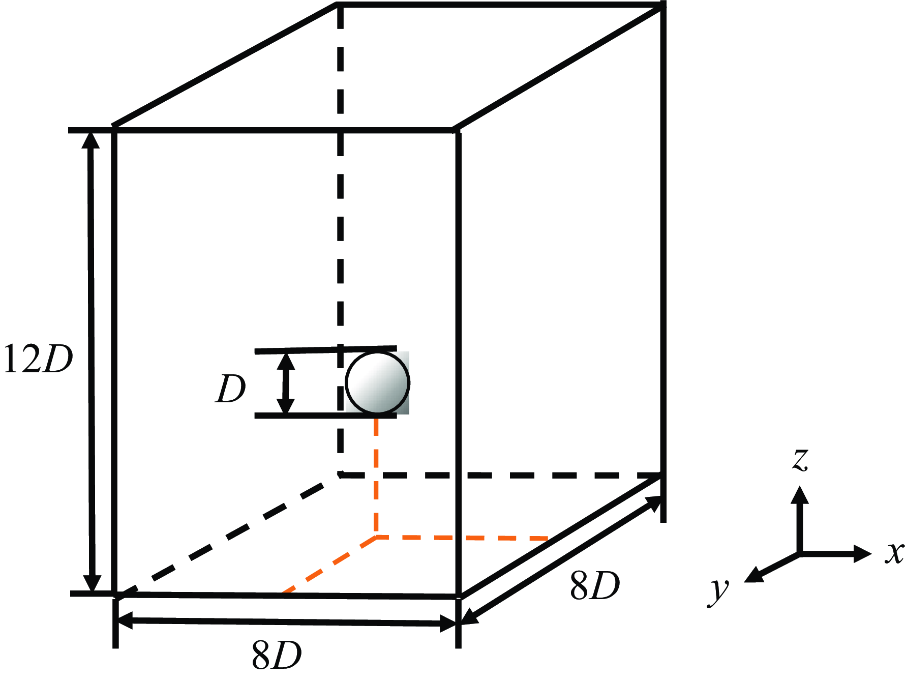
The accuracy of the three-dimensional phase-field method PINNs (PF-PINNs) was systematically evaluated using a three-dimensional bubble rising case study. This scenario involves a bubble rising in an infinitely large water tank under the influence of buoyancy, with the tank boundaries sufficiently distant from the bubble. When the bubble reached a constant terminal velocity, both the rising speed and the shape of the bubble were recorded and compared with experimental data to verify the accuracy of the results (Zhang, Sun & Ming Reference Zhang, Sun and Ming2015; Xu, Yang & Hu Reference Xu, Yang and Hu2023). The initial and boundary conditions for this case are depicted in figure 4. The spatial domain was defined as
 $V \in (x,y,z) \rightarrow [-1,1]\ \text{m}\times [-1,1]\ \text{m}\times[-1.5,1.5]\ \text{m}$
, and the time interval was set as
 $t \rightarrow [0,3]$
s. The initial position of the bubble’s centre was
 $(x_b,y_b,z_b) = (0,0, -0.5)$
m, with initial radius
 $r_b = 0.125$
m. The top and bottom boundaries of the domain are defined by wall boundary conditions, while the left, right, front and back boundaries are governed by slip boundary conditions. The distribution of the volume fraction field at the initial time
 $t=0$
is defined by the formula
 \begin{equation} C(x,y,z,t=0)=-\tanh\left(\frac {r_b-\sqrt {(x-x_b)^2+(y-y_b)^2+(z-z_b)^2}}{\sqrt {2}\epsilon }\right). \end{equation}
It is assumed that the entire field initially has zero velocity, and that the bubble rises vertically under the influence of buoyancy. The bubble, a circular gas region
 $G$
, is surrounded by liquid
 $L$
in a cuboid computational domain. As the bubble ascends, its shape undergoes changes. Once the velocity field stabilises, the shape of the bubble remains constant, allowing for the determination of the terminal rising velocity. The liquid density was set to
 $\rho _L = 1000 \, \rm {kg\,m}^{-3}$
, the gas density to
 $\rho _G = 1 \, \rm {kg\,m}^{-3}$
, the liquid viscosity to
 ${\rm \mu} _L = 8.161 \ \rm {N} \ \rm {s\ m}^{-2}$
, and the gas viscosity to
 ${\rm \mu} _G = 0.08161 \ \rm {N} \ \rm {s\ m}^{-2}$
. The ratios of density and viscosity between the liquid and gas were maintained at 1000 and 100, respectively. The value of the gravitational acceleration vector
 $\boldsymbol{g}$
was set to
 $(0, 0, -1) \, \rm {m\,s}^{-2}$
, indicating a direction towards the negative
 $z$
-axis. The surface tension coefficient at the liquid–as interface was
 $\sigma _0 = 0.25643 \, \rm {N\,m}^{-1}$
. The interface thickness and diffusion rate were set as
 $\epsilon = 6.25 \times 10^{-3} \, {\rm m}$
and
 $M_0=10^{-4} \ \rm{N\ m^{-1}\ s^{-1}}$
, respectively. In this scenario, the key dimensionless parameters to consider are the Bond number (
 $Bo$
), Morton number (
 $Mo$
) and Reynolds number (
 $Re$
). These numbers characterise the different flow regimes in the three-dimensional bubble rising case. The equations for calculating these dimensionless numbers are (Yang et al. Reference Yang, Rakhsha, Hu and Negrut2022)
 \begin{align} Bo &=\frac {(\rho _L-\rho _G) \Vert \boldsymbol g \Vert L^2}{\sigma _0}, \end{align}
 \begin{align} Mo &=\frac {\Vert \boldsymbol g \Vert\, {\rm \mu} ^4_L (\rho _L-\rho _G)}{\rho _L^2 \sigma _0^3}, \end{align}
 \begin{align} Re &=\frac {(\rho _L-\rho _G) U_{\infty } L}{{\rm \mu} _L}, \end{align}
Schematic representation of the initial and boundary conditions for the three-dimensional bubble rising case in infinite water. Here,
 $D$
denotes the diameter of the bubble,
 $D=2r_b$
.

where
 $L = 2r_b$
represents the characteristic length, typically considered as the diameter of the bubble, and
 $U_{\infty } = w_{\infty }$
is the terminal bubble rising velocity in the
 $z$
-direction when the bubble reaches a stable state. Yang et al. (Reference Yang, Rakhsha, Hu and Negrut2022) note that in cases with a small density ratio, the gas density cannot be ignored when calculating the Bond number. Although this study did not focus on small density ratio cases, the form of the Bond number that includes the gas density was retained. The values of these dimensionless numbers and the related variables are detailed in table 1.
Table of physical parameters and dimensionless numbers for the three-dimensional bubble rising case.

3.2. Implementing details of PINNs
The bubble rising case addresses the temporal span
 $t \rightarrow [0,3]$
s. In this case, we divides the time range into eleven intervals:
 $[0,0.25]$
s,
 $[0.25,0.5]$
s,
 $[0.5,0.75]$
s,
 $[0.75,1]$
s,
 $[1,1.25]$
s,
 $[1.25,1.5]$
s,
 $[1.5,1.75]$
s,
 $[1.75,2]$
s,
 $[2,2.25]$
s,
 $[2.25,2.5]$
s and
 $[2.5,2.75]$
s. Additionally, the domain decomposition method in the spatial domain is applied to accelerate the training of PF-PINNs. The spatial domain is partitioned into eight subdomains, each corresponding to a different GPU device, with the division occurring as two sections in the
 $x$
-direction, two in the
 $y$
-direction, and two in the
 $z$
-direction, as illustrated in figure 5. The overlap between each subdomain on the interface
 $\Delta W$
is set at 0.5 times the width of each subdomain, representing the dimensionless overlap width. The dimensionless overlapping boundary width setting is set according to our previous work (Qiu et al. Reference Qiu, Dong, Wang, Fan and Wang2024).
Schematic diagram of the domain decomposition method employed in the three-dimensional bubble rising case in infinite water.

To model the bubble rising process, fully connected neural networks comprising five residual blocks were utilised. Each residual block contains two fully connected layers, each of width 128 neurons, facilitating the input–output mapping from the sampled spatio-temporal coordinates
 $(x,y,z,t)$
to physical quantities such as velocity vectors, pressure, volume fractions and chemical potential
 $(C,u,v,w,p, \phi )$
. The AdamW optimisation method was employed, with the learning rate progressively reduced from
 $1\times 10^{-3}$
to
 $1\times 10^{-6}$
to ensure comprehensive training of the network. The loss function demonstrated a steady decrease throughout the training process, which involved a total of
 $1.8 \times 10^6$
iterations. Adjustment to hyperparameters, particularly concerning learning rate settings, are detailed in table 2. The sampling points for this analysis were derived from a spatially and temporally uniform grid prepared previously. Grid sizes in the
 $x$
-,
 $y$
- and
 $t$
-directions are
 $\Delta x = 0.00625$
m,
 $\Delta y = 0.00625$
m and
 $\Delta t = 0.0625$
s, respectively. The distribution of sampling points is as follows: each subnetwork samples 5000 initial points randomly at
 $t = 0$
s in each iteration, and 4000 boundary points at each spatial boundary (i.e.
 $N_{ICs} = 5000$
and
 $N_{BCs} = 4000$
), and 15 000 equation points are randomly selected within the computational domain.
Settings of the learning rate for the neural network in the three-dimensional bubble rising case.

In the hardware environment, both training and inference of the neural network were executed on a single compute node. However, the experiments for evaluating scalability of our algorithm were extended to multiple nodes. A node is equipped with eight NVIDIA Tesla V100-SXM2 GPUs, each with 32 GB of graphics memory. For efficient communication, high-bandwidth PCIe was utilised for intra-node communication, while a high-speed InfiniBand network was employed for inter-node communication. In the software environment, the Jax deep learning framework, version 0.4.13, was utilised, requiring CUDA library version 11.0. Double-precision training was employed to enhance the accuracy of derivative calculations during the neural network’s automatic differentiation process. To prevent CPU computation from becoming a bottleneck, each GPU was paired with 6 CPUs.
Sequence of three-dimensional bubble shapes at specified times: (a)
 $t=0$
s, (b)
 $t=0.5$
s, (c)
 $t=1$
s, (d)
 $t=1.5$
s, (e)
 $t=2$
s, (f)
 $t=2.5$
s.

Time variation of quantitative parameters in the three-dimensional bubble rising case: (a) centre of mass of the bubble; (b) rising velocity of the bubble.

3.3. Validation of accuracy and parametric study
Figure 6 depicts the evolution of the bubble interface in the three-dimensional bubble rising scenario at specific instances. Initially, the bubble ascends slowly from a stationary position along the centreline of the water tank, undergoing changes in shape. By
 $t = 2.5$
s, the bubble’s shape approaches stability, and its ascent rate can be considered the terminal rising velocity. To quantitatively assess the evolution of the bubble rising process, two parameters were defined: the centre of mass and the rising velocity of the bubble. These quantitative parameters were derived using the following expressions for the average
 $z$
-direction coordinate and the average
 $z$
-direction velocity of all sampling points within the bubble:
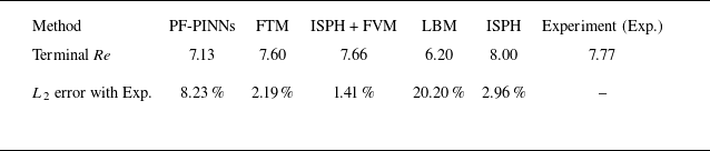
Comparison of terminal Reynolds numbers using various algorithms in the three-dimensional bubble rising case.

 \begin{align}&\qquad z_b(t) =\frac {\int _{V \in (x,y,z)}{z\dfrac{1-C(x,y,z,t)}{2}{\rm d}V}}{\int _{V \in (x,y,z)} {\dfrac{1-C(x,y,z,t)}{2} {\rm d}V}},\\[-7pt] \end{align}
 \begin{align}& w_b(t) =\frac {\int _{V \in (x,y,z)} {w(x,y,z,t) \dfrac{1-C(x,y,z,t)}{2} {\rm d}V}}{\int _{V \in (x,y,z)} \dfrac{1-C(x,y,z,t)}{2} {\rm d}V}, \end{align}
where
 $V$
denotes the computational domain at time
 $t$
. The resulting curves of these two quantitative parameters are displayed in figure 7. The data indicate that the rising velocity of the bubble initially increases, reaches a peak, and subsequently stabilises at the terminal velocity. The impact of the bubble’s shape on its rising velocity occurs in two phases: initially, the gravitational pull is the predominant force propelling the bubble upwards; as the bubble deforms, the increased surface tension eventually balances the gravitational force. Table 3 provides further comparisons of the Reynolds number at the point of terminal rising velocity with results from the front tracking method (FTM) from Hua, Stene & Lin (Reference Hua, Stene and Lin2008), incompressible smoothed particle hydrodynamics (ISPH) and finite-volume method (FVM) coupling (ISPH + FVM) from Xu et al. (Reference Xu, Yang and Hu2023), lattice Boltzmann method (LBM) from Cheng, Hua & Lou (Reference Cheng, Hua and Lou2010), ISPH from Yang et al. (Reference Yang, Rakhsha, Hu and Negrut2022), and experiment results (Exp.) from Bhaga & Weber (Reference Bhaga and Weber1981) when the terminal rising velocity of bubble is reached. These comparisons demonstrate that PINNs effectively simulate the three-dimensional bubble rising in infinite water under low Reynolds numbers, showing minimal deviation from experimental results.
Comparison of quantitative parameters in the bubble rising case for PF-PINNs among fine sampling points (1 20 000), medium sampling points (60 000) and coarse sampling points (30 000): (a) centre of mass of the bubble; (b) rising velocity of the bubble.

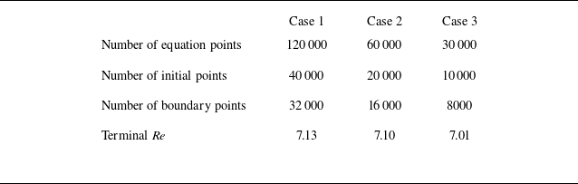
To evaluate the convergence of the training results, we conducted convergence tests by varying the number of sampling points and the spatial resolution of the background grid. For the number of sampling points, three configurations with 1 20 000, 60 000 and 30 000 equation points were selected for training the PINNs equations, while other types of sampling points were proportionally reduced. All other settings remained consistent with the previous case. The bubble rising velocity was used as the quantitative metric for evaluation. The average bubble rising velocity during
 $t = 2.5{-}2.75$
s was calculated, and the corresponding terminal Reynolds number derived from this velocity is summarised in figure 8 and table 4. The results demonstrate that as the number of sampling points increases, the terminal Reynolds number approaches convergence. For spatial resolution of the background grid, we choose three grid sizes,
 $\Delta x_1 = 0.00625$
m,
 $\Delta x_2 = 0.0125$
m and
 $\Delta x_3 = 0.003125$
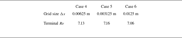
m. All other settings remained consistent with the previous case. The bubble rising velocities of PF-PINNs in three grid sizes are listed in table 5, demonstrating that the size of the background grid has minimal influence on the convergence process of PF-PINNs.
Comparison of terminal Reynolds numbers using various sampling points in the three-dimensional bubble rising case.

Comparison of terminal Reynolds numbers using various background grid sizes in the three-dimensional bubble rising case.

Existing studies have indicated that the phase-field model employed in this work may fail to satisfy the divergence-free condition
 $\boldsymbol{\nabla} \boldsymbol{\cdot} \boldsymbol u=0$
when solving incompressible two-phase flows with large density ratios, leading to convergence difficulties in the governing equations. The thermodynamically consistent phase-field method proposed by Abels et al. (Reference Abels, Garcke and Grun2012) resolves the problem by refining the convective term in the momentum equation. We rigorously derived momentum equations satisfying thermodynamic consistency principles, and reformulated them into the loss function of PINNs. The specific mathematical formulation is provided in Appendix D. Comparative analysis of bubble rising velocity between conventional and thermodynamics-consistent implementations is shown in figure 9, which indicates that the maximum deviation of terminal Reynolds numbers between conventional and thermodynamics-consistent PINNs is below 3 %, demonstrating that enforcing thermodynamic consistency conditions has no significant impact on final predictions in this specific bubble rising configuration.
Comparison of quantitative parameters in the bubble rising case between conventional and thermodynamics-consistent PINNs: (a) centre of mass of the bubble; (b) rising velocity of the bubble.

3.4. Discussions of computational time and parallel efficiency
To demonstrate the computational efficiency of the developed algorithm in three-dimensional two-phase flow scenarios, this subsection employs the same benchmark case as the preceding subsection to evaluate runtime performance and parallel scaling efficiency. The ISPH method is selected from table 3 as a representative state-of-the-art numerical algorithm for computational cost comparison. Yang et al. (Reference Yang, Rakhsha, Hu and Negrut2022) reported computational time 48 h on a single NVIDIA V100 GPU for their three-dimensional bubble rising case. The proposed method utilised eight NVIDIA V100 GPUs and required 297 h to complete the training of the three-dimensional bubble rising case across 11 temporal subintervals. The comparison of computational time between our method and the ISPH approach demonstrates that their computational durations are already comparable. With additional computational resources or further optimisation of the PINNs architecture, the computational time of the proposed PINNs framework could be substantially reduced.
The computational efficiency of the proposed parallel training algorithm was assessed rigorously. Following the definitions provided by Shukla et al. (Reference Shukla, Jagtap and Karniadakis2021) and Wang et al. (Reference Wang, Sankaran and Perdikaris2024b
), both weak and strong scalings on GPUs were assessed. The weak scaling efficiency
 $E_w$
is expressed as
 \begin{equation} E_w = \frac {t_1}{t_{N_p}}, \end{equation}
where
 $t_1$
is the time with a single GPU, and
 $t_{N_p}$
is the time required to complete the
 $N_p$
unit of the same work with
 $N_p$
GPUs. As depicted in figure 10(a), for convenience, the weak scaling defined by the processing of sampling points per GPU per second exhibited linear performance. This result is closely tied to our optimisation strategy of overlapping communication with computation. This demonstrates the potential of our approach to effectively address larger-scale problems.
Strong scalability measures the ability to achieve better acceleration performance as the number of GPUs increases while maintaining the same total problem size. The strong scaling effciency is expressed as
 \begin{equation} E_s = \frac {s}{N_p}, \end{equation}
where
 $s$
represents the speed-up, calculated as
 $s={t_1}/{t_{N_p}}$
, with
 $t_1$
the time with a single GPU, and
 $t_{N_p}$
the time taken to complete the same computation with
 $N_p$
GPUs. As shown in figure 10(b), the parallel efficiency gradually declines as the number of GPUs increases, and the speed-up achieves approximately 60 % with 16 GPUs. It is potential for improvement in the strong scaling performance of the GPU algorithm. The under-utilisation of each GPU may reduce its parallel efficiency, suggesting that further optimisation is possible. Continued research is needed to devise strategies that enhance scalability in the multi-GPU training environment of PINNs, potentially leading to more robust and efficient computational frameworks.
Assessment of parallel training performance on multiple GPUs: (a) weak scaling of the proposed method; (b) strong scaling, including speed-up and efficiency of the proposed method.

4. Concluding remarks
Current research on PINNs related to two-phase flows has predominantly focused on two-dimensional models, which do not fully meet the needs of real-world physical problems and engineering applications. In this study, we expanded our investigation to explore the feasibility of employing PF-PINNs for direct numerical simulations of three-dimensional two-phase flows. The three-dimensional implementation of PF-PINNs utilised a distributed parallel training algorithm across multiple GPUs , incorporating a fully connected neural network with residual blocks. We selected a bubble rising case in infinite water as a classical benchmark to evaluate the reliability of the proposed method. Comparative analysis between the proposed PF-PINNs framework, conventional numerical result and experimental data demonstrates that our method can accurately model the entire process of three-dimensional two-phase flow, yielding precise quantitative parameters such as the terminal Reynolds number. The relative error in the terminal Reynolds number, when compared to experimental results, was approximately 8.23 %, confirming the accuracy of our framework. Meanwhile, we systematically analysed the effects of sampling points number, background grid resolution, and modified phase-field equations on the computational results of PINNs, demonstrating the reliability of the solution methodology employed in this work. Furthermore, the computational time and parallel training efficiency of the developed PINNs was evaluated across multiple GPUs, demonstrating robust scaling capabilities, which are crucial for achieving large-scale distributed parallel training with extensive sampling points.
The distributed parallel training algorithm exhibited strong performance under weak scaling conditions, supporting the use of increased numbers of sampling points across more GPU devices. The proposed framework successfully addresses the challenges associated with training surrogate models for three-dimensional two-phase flows, and exhibits significant potential for engineering applications across a range of two-phase flow problems. Future efforts could focus on a series of enhancements, including loss term balancing strategies, adaptive sampling strategy on the domain decomposition method for refining complex interfaces, and network architectures incorporating Fourier features for high-frequency flow fields, to further enhance the computational accuracy of the algorithm.
Funding
This work was supported by the National Natural Science Foundation of China (nos 12293003, 12525210, 12293000, 12272382, 52441101) and the Youth Innovation Promotion Association CAS (2022019).
Declaration of interests
The authors report no conflict of interest.
Data availability
The data that support the findings of this study are openly available in Github at https://github.com/misaka-pikapika/PF-PINNs-three-dimensional.
Appendix A. Loss function of PF-PINNs in three-dimensional two-phase flow
The residual formulations of the continuity equation (2.3), interface evolution equation (2.5) and momentum equations in the x-, y- and z-directions (2.4) are represented by
 $L_M, L_C, L_U, L_V, L_W, L_{\phi }$
. The construction of each loss function is detailed as follows:
 \begin{align}&\qquad\qquad\qquad\qquad\qquad\quad L_{{M}} =u_x+v_y+w_z, \end{align}
 \begin{align}&\qquad\qquad L_C =C_t+u C_x+v C_y+w C_z - M_0(\phi _{xx}+\phi _{yy}+ \phi _{zz}), \end{align}
 \begin{align} L_U &= (\rho _{{M}} (u_t + u u_x + v u_y+ w u_z)+p_x - 0.5 ({\mu} _{{L}}-{\mu} _{{G}}) C_y (u_y+v_x) \nonumber\\ & \quad -({\mu} _{{L}}-{\mu} _{{G}})C_x u_x - 0.5 ({\mu} _{{L}}-{\mu} _{{G}}) C_z (u_z +v_w)-{\mu} _{{M}}(u_{xx}+u_{yy}+u_{zz} ) \nonumber\\ & \quad -f_{\sigma x} -\rho _{{M}} g_x)/\rho _{{L}}, \end{align}
 \begin{align} L_V &= (\rho _{{M}} (v_t + u v_x + v v_y + w v_z)+ p_y - 0.5 ({\rm \mu} _{{L}}-{\rm \mu} _{{G}})C_x (v_x+u_y) \nonumber\\ &\quad - ({\rm \mu} _{{L}}-{\rm \mu} _{{G}}) C_y v_y -0.5 ({\rm \mu} _{{L}}-{\rm \mu} _{{G}})C_z (v_z+w_y) -{\rm \mu} _{{M}}(v_{xx}+v_{yy}+v_{zz}) \nonumber\\ &\quad -f_{\sigma y} -\rho _{{M}} g_y)/\rho _{{L}}, \end{align}
 \begin{align} L_W &= (\rho _{{M}} (w_t + u w_x + v w_y+ w w_z)+p_z-0.5 ({\rm \mu} _{{L}}-{\rm \mu} _{{G}})C_x(w_x+u_z) \nonumber\\ &\quad - ({\rm \mu} _{{L}}-{\rm \mu} _{{G}}) C_z w_z -0.5 ({\rm \mu} _{{L}}-{\rm \mu} _{{G}})C_y(v_z+w_y)-{\rm \mu} _{{M}}(w_{xx}+w_{yy}+w_{zz}) \nonumber\\ &\quad -f_{\sigma z} -\rho _{{M}} g_z)/\rho _{{L}}, \end{align}
 \begin{align}&\qquad\qquad L_{\phi } = \phi - \big(C(C^2-1)-\epsilon ^2(\phi _{xx}+\phi _{yy}+\phi _{zz})\big). \end{align}
The equation loss function of the neural network is calculated by aggregating the individual loss functions derived from the equations mentioned above. The discrete representations of the governing equations are
 \begin{align} L_{Eqn} &=L_{{M}}+L_C+L_U+L_V+L_W+L_{\phi }, \end{align}
 \begin{align} L_{Eqn} &= \frac {1}{N_{Eqn}}\sum _{j=1}^{N_{Eqn}} \left(\left|L_{C}\left(X_{Eqn}^j\right)\right|^2+\left|L_{U}\left(X_{Eqn}^j\right)\right|^2+\left|L_{V}\left(X_{Eqn}^j\right)\right|^2\right . \nonumber\\ &\quad\left .+\,\left|L_{W}\left(X_{Eqn}^j\right)\right|^2 +\left|L_{M}\left(X_{Eqn}^j\right)\right|^2+\left|L_{\phi }\left(X_{Eqn}^j\right)\right|\right), \end{align}
where
 $L_{Eqn}$
denotes the discretised governing equations. The terms
 $X_{Eqn}^j=(x_{Eqn}^j, y_{Eqn}^j, z_{Eqn}^j, t_{Eqn}^j)$
refer to the
 $j$
th sampling points in the internal fields. The parameters for constructing
 $L_{Eqn}$
are calculated via
 $(C_{Eqn}^j,u_{Eqn}^j,v_{Eqn}^j,w_{Eqn}^j,p_{Eqn}^j,\phi _{Eqn}^j)=F_{NN}(X_{Eqn}^j;\Theta )$
. The numbers of these sampling points are designated as
 $N_{Eqn}$
for the internal fields.
In three-dimensional two-phase flow PINNs, there typically exist six boundary conditions, corresponding to top, bottom, right, left, front and back boundaries. Since the proposed PINNs framework incorporates a spatial domain decomposition method, each subdomain generally requires first determining the boundary type associated with each boundary before formulating the specific expression of the boundary loss. Regardless of the specific boundary type, given the
 $j$
th boundary points
 $X_{BCs-k}^j=(x_{BCs-k}^j,y_{BCs-k}^j,z_{BCs-k}^j,t_{BCs-k}^j)$
on boundary
 $k\in \{\text{N, S, E, W, U, D}\}$
, the corresponding loss function can always be expressed in the form
 \begin{align} L_{BCs} &= \frac {1}{N_{BCs}}\sum _k \sum _{j=1}^{N_{BCs}} \left(\left|C_{BCs-k}^j-C_k\right|^2+\left|u_{BCs-k}^j-u_k\right|^2+\left|v_{BCs-k}^j-v_k\right|^2 \right. \nonumber\\&\quad \left. +\, \left|w_{BCs-k}^j-w_k\right|^2 \right), \end{align}
where
 $L_{BCs}$
denotes the discretised boundary conditions. The parameters for constructing
 $L_{Bcs}$
are calculated via
 $(C_{BCs-k}^j,u_{BCs-k}^j,v_{BCs-k}^j,w_{BCs-k}^j,\ldots )=F_{NN}(X_{BCs-k}^j;\Theta )$
. The numbers of these sampling points are designated as
 $N_{BCs}$
for the boundary fields. The specific formulation of
 $(C_k,u_k,v_k,w_k)$
is determined in Appendix B.
Due to the implementation of the time-marching strategy in this work, the initial conditions for the neural networks are no longer determined by physical quantities at
 $t = 0$
, but rather are determined by the output from the neural network of the preceding time interval. Similarly, while no explicit analytical form can be prescribed, the loss function for initial conditions follows a structure analogous to that of the boundary conditions. For
 $N_t$
sequential time intervals, given the
 $j$
th initial condition points
 $X_{ICs-l}^j=(x_{ICs-l}^j,y_{ICs-l}^j,z_{ICs-l}^j,t_{ICs-l}^j)$
on the
 $l$
th time interval (
 $l\in \{1,2,\ldots ,N_t\}$
), the corresponding loss term can always be expressed as
 \begin{align} L_{ICs}&= \frac {1}{N_{ICs}} \sum _{j=1}^{N_{ICs}} \Big(\big|C_{ICs-l}^j-C_l\big|^2+\big|u_{ICs-l}^j-u_l\big|^2+\big|v_{ICs-l}^j-v_l)\big|^2\nonumber \\&\quad +\big|w_{ICs-l}^j-w_l\big|^2 \Big), \end{align}
where
 $L_{ICs}$
denotes the discretised initial conditions. The parameters for constructing
 $L_{ICs}$
are calculated via
 $(C_{ICs-l}^j,u_{ICs-l}^j,v_{ICs-l}^j,w_{ICs-l}^j,\ldots )=F_{NN}(X_{ICs-l}^j;\Theta )$
. The numbers of these sampling points are designated as
 $N_{ICs}$
for the boundary fields. The specific formulation of
 $(C_l,u_l,v_l,w_l)$
is determined in Appendix C. The total loss function of the neural network is calculated by aggregating the individual loss functions derived from the equations mentioned above, in addition to the loss functions associated with the initial and boundary conditions. Thus we have
 \begin{equation} L_{total}=L_{Eqn}+L_{ICs}+L_{BCs}. \end{equation}
Appendix B. Initial condition of PINNs using the time-marching strategy
In the time-marching strategy, the initial condition for the
 $l$
th neural network is determined solely by the
 $(l-1)$
th neural network. The initial condition for the first neural network, however, is prescribed by the initial values of the physical problem, leading to
 $C_0=C(x,y,z,t=0)$
,
 $u_0=0$
m s–1,
 $v_0=0$
m s–1 and
 $w_0=0$
m s–1. Thus the expression for the initial condition of the
 $l$
th neural network can be readily derived as
 \begin{align} &\qquad (C_{prev},u_{prev},v_{prev},w_{prev},\ldots )=F_{NN}(X_{ICs-(l-1)};\Theta _{prev}), \end{align}
 \begin{align} C_l &=\begin{cases} C(x,y,z,t=0),\ u_l=0 \ {\rm m\ s^{-1}},\ v_l=0 \ {\rm m\ s^{-1}},& \!\!\!\!\!w_l=0 \ {\rm m\ s^{-1}}, l=0,\\ C_{prev},\ u_l=u_{prev},\ v_l=v_{prev},\ w_l=w_{prev},& \!\!\!\!\!\!\!\!\! l\gt 0. \end{cases} \end{align}
Appendix C. Boundary condition of PINNs with the domain decomposition method
In the domain decomposition method, each subdomain requires training the corresponding subnetwork using the loss function defined in Appendix A. For the six boundary conditions within each subdomain, the boundary type must first be determined. The boundary conditions are classified into two categories.
Overlapping boundary conditions: boundaries shared with adjacent subdomains. These only require consistency between the current subnetwork’s output and that of neighbouring subnetworks. The specific forms of the target parameters
 $(C_k,u_k,v_k,w_k)$
can be defined as
 \begin{align} &\qquad\quad\,\,(C_{adj},u_{adj},v_{adj},w_{adj},\ldots ) =F_{NN}(X_{BCs-k};\Theta _{adj}), \end{align}
 \begin{align} & C_k =C_{adj},\, u_k=u_{adj},\, v_k=v_{adj},\, w_k=w_{adj},\, k\in \{\textrm {N, S, E, W, U, D}\}. \end{align}
Physical boundary conditions: boundaries not overlapping with any subdomain. In the bubble rising case in infinite water, the top and bottom boundaries enforce no-slip wall conditions, leading to
 $C=1$
and
 $\boldsymbol u=(0,0,0)\ \textrm {m s}^{-1}$
, while the front, back, right and left boundaries enforce free-slip conditions, leading to
 $C=1$
,
 $\boldsymbol u \boldsymbol{\cdot} \boldsymbol n=0$
and
 ${\partial \boldsymbol u}/{\partial \boldsymbol n}=0$
, where
 $\boldsymbol n$
denotes the normal vector of physical boundary conditions. The specific forms of the target parameters
 $(C_k,u_k,v_k,w_k)$
for each boundary type are derived as
 \begin{align} &\qquad\quad (\ldots ,v_{BCs-k \pm x},w_{BCs-k \pm x},\ldots )=F_{NN}(X_{BCs-k} \pm \Delta x;\Theta _{local}), \end{align}
 \begin{align} &\qquad (\ldots ,u_{BCs-k \pm y},\ldots ,w_{BCs-k \pm y},\ldots )=F_{NN}(X_{BCs-k} \pm \Delta y;\Theta _{local}), \end{align}
 \begin{align} & \begin{cases} C_N=1,\,u_N=u_{BCs-N+y},\,v_N=0 \, {\rm m\,s^{-1}},\,w_N=w_{BCs-N+y},\quad \textrm {when N in front},\\ C_S=1,\,u_S=u_{BCs-S-y},\,v_S=0 \, {\rm m\,s^{-1}},\,w_S=w_{BCs-S-y},\quad \textrm {when S in back},\\ C_E=1,\,u_E=0 \, {\rm m\,s^{-1}},\,v_E=v_{BCs-E-x},\,w_E=w_{BCs-E-x}, \quad \textrm {when E in right},\\ C_W=1,\,u_W=0 \, {\rm m\,s^{-1}},\,v_W=v_{BCs-W+x},\,w_W=w_{BCs-W+x}, \quad \textrm{when W in left},\\ C_U=1,\,u_U=0 \, {\rm m\,s^{-1}},\,v_U=0 \, {\rm m\,s^{-1}},\,w_U=0 \, \, {\rm m\,s^{-1}},\quad \textrm {when U in top},\\ C_D=1,\,u_D=0 \, {\rm m\,s^{-1}},\,v_D=0 \, {\rm m\,s^{-1}},\,w_D=0 \, \, {\rm m\,s^{-1}},\quad \textrm {when D in bottom}. \end{cases} \end{align}
Appendix D. Improvement of PINNs with the thermodynamically consistent phase-field method
Compared to the conventional phase-field formulation, the thermodynamically consistent phase-field method introduces a corrective term into the convective component of the momentum equation. The modified governing equation is derived from (2.4) and can be expressed as
 \begin{equation} \frac {\partial \left (\rho u_i \right )}{\partial t}+\frac {\partial \left (m_j u_i \right )}{\partial x_j}= -\frac {\partial p}{\partial x_i}+\frac {\partial }{\partial x_j}\left [{\rm \mu} _M \left (\frac {\partial u_i}{\partial x_j}+\frac {\partial u_j}{\partial x_i} \right ) \right ]+\frac {3\sqrt {2}}{4}\frac {\sigma _0}{\epsilon }\phi \frac {\partial C}{\partial x_i}+\rho _M g_i, \end{equation}
where indices
 $i$
and
 $j$
denote tensor notation,
 $m_i=\rho u_i - ({(\rho _L-\rho _G)}/{2})M_0({\partial \phi }/{\partial x_i})$
, and
 $ {\partial m_i}/{\partial x_i}= - (({\rho _L-\rho _G})/{2})M_0({\partial ^2 \phi }/{\partial x_i^2})$
. Expanding (D1) while enforcing the continuity constraint
 $({\partial u_i}/{\partial x_i})=0$
, the modified momentum equation’s loss function formulation is expressed as
 \begin{align} L_U^* &= \biggl(\rho _{{M}} (u_t + m_x u_x + m_y u_y+ m_z u_z) - \frac {\rho _L-\rho _G}{2}M_0 u (\phi _{xx}+\phi _{yy}+\phi _{zz}) + p_x \nonumber\\ &\quad -0.5 ({\rm \mu} _{{L}}-{\rm \mu} _{{G}}) C_y (u_y+v_x)-({\rm \mu} _{{L}}-{\rm \mu} _{{G}})C_x u_x- 0.5 ({\rm \mu} _{{L}}-{\rm \mu} _{{G}}) C_z (u_z +v_w) \nonumber\\ &\quad -{\rm \mu} _{{M}}(u_{xx}+u_{yy}+u_{zz} )-f_{\sigma x}-\rho _{{M}} g_x\biggr)/\rho _{{L}}, \end{align}
 \begin{align} L_V^* &= \biggl(\rho _{{M}} (v_t + m_x v_x + m_y v_y+ m_z v_z) - \frac {\rho _L-\rho _G}{2}M_0 v (\phi _{xx}+\phi _{yy}+\phi _{zz})+ p_y \nonumber\\ &\quad -0.5 ({\rm \mu} _{{L}}-{\rm \mu} _{{G}})C_x (v_x+u_y)- ({\rm \mu} _{{L}}-{\rm \mu} _{{G}}) C_y v_y -0.5 ({\rm \mu} _{{L}}-{\rm \mu} _{{G}})C_z (v_z+w_y) \nonumber\\ &\quad -{\rm \mu} _{{M}}(v_{xx}+v_{yy}+v_{zz})-f_{\sigma y}-\rho _{{M}} g_y\biggr)/\rho _{{L}}, \end{align}
 \begin{align} L_W^* &= \biggl(\rho _{{M}} (w_t + m_x w_x + m_y w_y+ m_z w_z) - \frac {\rho _L-\rho _G}{2}M_0 w (\phi _{xx}+\phi _{yy}+\phi _{zz})+p_z \nonumber\\ &\quad -0.5 ({\rm \mu} _{{L}}-{\rm \mu} _{{G}})C_x(w_x+u_z)- ({\rm \mu} _{{L}}-{\rm \mu} _{{G}}) C_z w_z -0.5 ({\rm \mu} _{{L}}-{\rm \mu} _{{G}})C_y(v_z+w_y) \nonumber\\ &\quad -{\rm \mu} _{{M}}(w_{xx}+w_{yy}+w_{zz})-f_{\sigma z}-\rho _{{M}} g_z\biggr)/\rho _{{L}}. \end{align}
Replacing (A3), (A4) and (A5) with (D2), (D3) and (D4), respectively, the loss function of PF-PINNs with thermodynamic consistency is obtained.