





1. Introduction
Turbulent boundary layers (BLs) experiencing streamwise pressure gradients are widespread in various engineering applications. Despite their significance, it remains difficult to model the impact of pressure gradients on the characteristics of wall-bounded turbulence. Given that the effect of pressure gradients on turbulent BLs closely relates to their streamwise development, it is crucial to examine the concept of equilibrium. According to Townsend's idealized definition (Townsend Reference Townsend1956), equilibrium is attained when all flow properties achieve self-similarity based on a consistent set of scaling variables, rendering the normalized flow independent of streamwise position. Self-similarity implies that profiles of a specific flow parameter measured at different locations exhibit identical shapes and can be collapsed onto a single form through appropriate normalization. The requirement for absolute equilibrium can be relaxed by semi-equilibrium (or approximate equilibrium) (Devenport & Lowe Reference Devenport and Lowe2022), which denotes a condition where the normalized flow changes gradually with streamwise position over distances much greater than the BL thickness, often due to Reynolds number dependence.
In the context of a statistically two-dimensional turbulent BL with a non-zero pressure gradient, the relative state of equilibrium can be quantified using the non-equilibrium Clauser parameter (Clauser Reference Clauser1954),  $\beta$. The constraint of constant
 $\beta$ is assumed to be necessary to approach (approximate) equilibrium in BL flows (Devenport & Lowe Reference Devenport and Lowe2022). Using the von Kármán momentum integral equation (von Kármán Reference von Kármán1921),
 $\beta$ may be interpreted as the ratio between the excess streamwise pressure force applied on the BL (relative to potential flow solution) and the wall shear stress (
 $\tau _w$). It is important to note that while a constant
 $\beta$ is a prerequisite for equilibrium behaviour, turbulent BLs, even in zero-pressure-gradient (ZPG) scenarios, are not completely similar due to the inherent independence of the inner and outer flow scales. The potential for an equilibrium state in turbulent BLs under pressure gradients can be illustrated through similarity analyses (Castillo & George Reference Castillo and George2001; Devenport & Lowe Reference Devenport and Lowe2022).
The presence of pressure gradients, whether adverse or favourable, serves as a source of non-equilibrium, thereby influencing the dynamics and behaviour of turbulent BLs. The large-scale motions in the outer region have been observed to be sensitive to pressure-gradient effects. For instance, Harun et al. (Reference Harun, Monty, Mathis and Marusic2013) used spectral and scale decomposition analysis to observe that the turbulent large structures are more energetic under the adverse-pressure-gradient (APG) effects. Despite being more energized, they observed a similar spectral distribution of energy within the wake region of the flow, indicating that the geometrical structure of the outer layer remains universal.
In BLs subjected to imposed APGs, deviations of the mean velocity profile within the logarithmic region were observed for both approximate equilibrium (constant  $\beta$) and non-equilibrium (Monty, Harun & Marusic Reference Monty, Harun and Marusic2011; Bobke et al. Reference Bobke, Vinuesa, Örlü and Schlatter2017) flows. Additionally, the impact of APG on the stronger wake region has been documented (Durbin & Belcher Reference Durbin and Belcher1992). Bobke et al. (Reference Bobke, Vinuesa, Örlü and Schlatter2017) further analysed the effect of APG on Reynolds stress components through a series of high-fidelity numerical experiments on flat plates and the suction side of an airfoil. They observed that inner-scaled Reynolds stress components increase with higher levels of
 $\beta$. Specifically, the streamwise normal Reynolds stress develops a secondary peak within the outer layer, a peak that amplifies at higher
 $\beta$. On the other hand, the strength and location of the inner peak remain unchanged. Moreover, an APG leads to a significant enhancement of the Reynolds shear stress within the outer layer, resulting in an increase in correlation between streamwise and wall-normal velocities and indicating a shift in the location and mechanism of turbulent production of kinetic energy (Skaare & Krogstad Reference Skaare and Krogstad1994). Adverse pressure gradients have been observed to reduce the number of low-speed streaks within the viscous sublayer while increasing the distance (Lee & Sung Reference Lee and Sung2009). In addition, the frequency of bursts in the inner region is reduced compared to ZPG BLs, whereas the frequency of sweep events is increased (Krogstad & Skåre Reference Krogstad and Skåre1995). As discussed above, the impact of APG on the outer region of the BL is more substantial. Within the outer region, the presence of trains of hairpin vortical structures and elongated low-momentum regions becomes more prominent compared with ZPG BLs (Lee & Sung Reference Lee and Sung2009).
While APGs have received considerable attention in research, there is comparably fewer studies focusing on favourable pressure gradients (FPG). Such FPGs entail flow acceleration in the flow's principal direction, resulting in a thinning of the BL thickness. If a strong FPG is imposed on turbulent BLs at sufficiently low Reynolds number, a reversion of the BL to a laminar state can result, as described by Narasimha & Sreenivasan (Reference Narasimha and Sreenivasan1973). Early experimental evidence of flow relaminarization under free-stream acceleration was shown by Sternberg (Reference Sternberg1955) on flow past a cone. However, in this work, the focus is limited to low-speed BLs, i.e. the incompressible regime. As elucidated by Narasimha & Sreenivasan (Reference Narasimha and Sreenivasan1973), the relaminarization process entails the suppression of turbulence to such an extent that the influence of Reynolds shear stresses on the mean flow significantly decreases. Consequently, the mean velocity profile deviates from the law of the wall and the skin friction coefficient may even decrease despite the free-stream acceleration. Patel (Reference Patel1965) observed deviations in the streamwise velocity profile beyond the logarithmic region, a finding subsequently corroborated by other studies (Wu & Squires Reference Wu and Squires1998; Matai & Durbin Reference Matai and Durbin2019). During the relaminarization process, turbulent intensity may not necessarily decrease; the production rate of turbulent kinetic energy can remain higher than its dissipation. However, the dominance of pressure forces due to flow acceleration leads the Reynolds stress components to become frozen, rendering them irrelevant to the flow dynamics. Hence, the term ‘quasi-laminar’ is used by Narasimha & Sreenivasan (Reference Narasimha and Sreenivasan1973) to characterize this flow state.
Several parameters have been proposed to quantify and predict relaminarization under FPGs. Patel (Reference Patel1965) introduced a parameter to define the relaminarization threshold using the FPG normalized by friction (inner) scaling for the breakdown of the logarithmic law. The threshold value was later revised by Patel & Head (Reference Patel and Head1968), and it was suggested that the non-dimensional shear stress gradient can offer a more universal criterion. Bradshaw (Reference Bradshaw1969) later revised the proposed value of the dimensionless shear stress gradient and suggested that it signifies the beginning of the logarithmic law overshoot rather than the initiation of the relaminarization process.
In aerodynamics and hydrodynamics applications, it is common for a BL to experience a FPG region followed by an APG region. The effects of an upstream FPG region on APG turbulent BLs were experimentally investigated in flows over bumps and hills both experimentally (Tsuji & Morikawa Reference Tsuji and Morikawa1976; Baskaran, Smits & Joubert Reference Baskaran, Smits and Joubert1987, Reference Baskaran, Smits and Joubert1991; Webster, DeGraaff & Eaton Reference Webster, DeGraaff and Eaton1996) and numerically (Wu & Squires Reference Wu and Squires1998; Matai & Durbin Reference Matai and Durbin2019). Uzun & Malik (Reference Uzun and Malik2018) simulated turbulent BL flow over a wall-mounted hump using a wall-resolved large-eddy simulation (WRLES) and compared the trend in the skin friction with the experimental results of Greenblatt et al. (Reference Greenblatt, Paschal, Yao, Harris, Schaeffler and Washburn2006). Additionally, they examined relaminarization under FPGs using a relaminarization parameter and concluded this process was incomplete at the Reynolds number they investigated. In a similar investigation, Balin & Jansen (Reference Balin and Jansen2021) conducted a direct numerical simulation (DNS) of low-speed flow over a two-dimensional Gaussian bump to examine the effects of alternating APG and FPG. Consistent with prior studies, they observed deviations from the logarithmic law due to FPG effects and reported their own threshold values to characterize the relaminarization process. Additionally, they observed the emergence of two internal layers resulting from the curvature changes on the bump surface, similar to the observation of Baskaran et al. (Reference Baskaran, Smits and Joubert1987). The formation of distinct internal layers within the BL suggests a decoupling between the inner and outer regions of the flow in non-equilibrium turbulent BLs. This phenomenon was further evidenced by recent numerical simulations conducted by Uzun & Malik (Reference Uzun and Malik2022) and Prakash et al. (Reference Prakash, Balin, Evans and Jansen2024) on a Gaussian bump at a larger Reynolds number, where they observed an internal layer created in the FPG region behaving similarly to a free shear layer. The internal layer near the wall behaves as a regular BL and is responsible for generating wall shear stress. Yet, far from the wall, flow behaves similarly to a free-shear flow, as described by Baskaran et al. (Reference Baskaran, Smits and Joubert1987), influenced by local pressure gradients and surface curvature (Balin & Jansen Reference Balin and Jansen2021).
The generation of internal layers due to alternating FPG and APG pertains to the flow history effects, which describe how upstream pressure gradients alter the turbulent statistics downstream. These history effects are known to prevent similarity in inner-scaled statistics, representing a challenge in developing robust turbulent models for non-equilibrium BLs (Prakash et al. Reference Prakash, Balin, Evans and Jansen2024). Bobke et al. (Reference Bobke, Vinuesa, Örlü and Schlatter2017) examined the history effects for APG BLs by comparing the inner-scaled mean velocity and Reynolds stress components of two distinct BLs with matching  $\beta$ and Reynolds number based on the friction velocity. They found that large structures within the outer layer are less energetic under APG if the upstream pressure gradients throughout their streamwise development are weaker. Additionally, their study suggested that the friction Reynolds number appears to inadequately capture the non-equilibrium effects. However, the choice of a Reynolds number based on displacement thickness and edge velocity yields more robust similarity for two distinct BLs.
Given the role of the momentum integral equation in establishing the physical meaning of the Clauser parameter,  $\beta$, it is worthwhile to investigate how integral equations can be utilized to further our understanding of pressure-gradient effects on turbulent BLs. For instance, turbulence is not explicitly represented in the momentum integral equation, even though it plays a significant role in the response of BLs to APGs, to the point of significantly altering incipient separation. Elnahhas & Johnson (Reference Elnahhas and Johnson2022) introduced the angular momentum integral (AMI) equation as an exact relationship between the Reynolds shear stress and the enhancement of BL skin friction relative to a baseline laminar BL. Thus, the AMI equation effectively accomplishes for BLs what the FIK equation (Fukagata, Iwamoto & Kasagi Reference Fukagata, Iwamoto and Kasagi2002) provides for internal turbulent flows such as pipe flow and channel flow. The analysis of Elnahhas & Johnson (Reference Elnahhas and Johnson2022), as well as subsequent work related to the AMI equation, focused on flat-plate ZPG BLs to elucidate skin friction and heat transfer during transition to turbulence (Kianfar, Elnahhas & Johnson Reference Kianfar, Elnahhas and Johnson2023b) and in supersonic BLs (Kianfar et al. Reference Kianfar, Di Renzo, Williams, Elnahhas and Johnson2023a). The natural capability of the AMI equation to include pressure-gradient effects in turbulent BL analysis has yet to be investigated in detail.
In this paper, the AMI equation is explored in the context of FPG and APG turbulent BLs and applied to simulation datasets to illuminate the interaction between BL turbulence and imposed pressure gradients. The outline of the paper is as follows. Section 2 surveys the theoretical background for the AMI equation, with particular attention to the treatment of terms related to the pressure gradient. In particular, the AMI equation is shown to define a modified Clauser-like parameter with a clear interpretation in terms of skin friction modification by pressure gradients in competition with turbulent stresses. Section 3 introduces the numerical simulation datasets that are explored in detail in § 4. The simulations include flow past a NACA 4211 airfoil at 5 $^\circ$ angle of attack (Vinuesa et al. Reference Vinuesa, Negi, Atzori, Hanifi, Henningson and Schlatter2018) and flow over a Gaussian bump (Balin & Jansen Reference Balin and Jansen2021). These datasets are explored individually using the AMI equation before investigating FPG and APG effects separately, including history effects. Conclusions are drawn in § 5.
2. Derivation and interpretation of the AMI equation
In this section, the derivation of the AMI equation is reviewed and adapted into a form most suitable for investigating how fully turbulent BLs react to non-zero pressure gradients. The derivation of the AMI equation is based on wall-normal integration of the transport equation for mean streamwise velocity defect,  $U - \bar {u}$. In the present notation, uppercase symbols are used to denote the free-stream flow solution in the absence of the BL and lowercase symbols are used for the physical flow solution. Allowing for turbulence within the BL, the overbar denotes a Reynolds average. The velocity defect represents the local deficit of momentum (or mass flux) within the BL. It decays rapidly to zero outside the BL and thus provides an integrable quantity in infinite and semi-infinite domains.
The scope of this paper is focused on (statistically) two-dimensional flows, although the concepts and procedures may be readily extended to general three-dimensional flows. The free-stream flow is described by the incompressible Euler equations:
 \begin{gather} \frac{\partial U}{\partial x} + \frac{\partial V}{\partial y} = 0, \end{gather}
 \begin{gather}\frac{\partial U}{\partial t} + U \frac{\partial U}{\partial x} +V \frac{\partial U}{\partial y} ={-}\frac{{\rm d} P}{{\rm d}\kern0.7pt x}. \end{gather}
In this study,  $x$ and
 $y$ denote the streamwise (wall-tangential) and wall-normal directions, respectively. For simplicity, the geometrical curvature effects (due to coordinate transformation) are not included in this derivation, and are generally negligible in the analysis performed in this paper (see Appendix A). The variables
 $U(x,y)$ and
 $V(x,y)$ denote the streamwise and wall-normal velocity in the absence of the BL, with (kinematic) pressure
 $P(x,y)$. In the presence of free-stream pressure gradients, the free-stream velocity may vary with wall-normal distance, though the variation across the thickness of an (attached) BL is typically small.
The flow given by  $U$ does not satisfy the no-slip boundary condition (BC). Instead, it may be considered either that the flow is inviscid (such that one fewer BC is needed), or that the no-slip BC is replaced by a different BC which does not introduce non-zero vorticity, so that
 $\varOmega = {\partial V}/{\partial x}-{\partial U}/{\partial y}=0$ everywhere in the domain. This irrotational assumption may be relaxed if desired. Additionally, it is assumed that there is no turbulence (zero Reynolds stress) in the absence of the BL.
Within the BL, the Reynolds-averaged Navier–Stokes (RANS) equations describe the flow:
 \begin{gather} \frac{\partial \bar{u}}{\partial x}+\frac{\partial \bar{v}}{\partial y}=0, \end{gather}
 \begin{gather}\frac{\partial \bar{u}}{\partial t}+\bar{u} \frac{\partial \bar{u}}{\partial x}+\bar{v} \frac{\partial \bar{u}}{\partial y}={-}\frac{\partial \bar{p}}{\partial x}+\nu \left(\frac{\partial ^2 \bar{u}}{\partial x^2} + \frac{\partial ^2 \bar{u}}{\partial y^2} \right)-\frac{\partial \overline{u^{\prime} u^{\prime}}}{\partial x}-\frac{\partial \overline{u^{\prime} v^{\prime}}}{\partial y}. \end{gather}
In these equations,  $\nu$ denotes the fluid kinematic viscosity,
 $\bar {u}(x,y)$ and
 $\bar {v}(x,y)$ represent the mean streamwise and wall-normal velocities, respectively, and
 $\bar {p}$ is the mean pressure (divided by density).
Subtracting the RANS  $x$-momentum equation, (2.4), from that of the free-stream flow, (2.2), and adding
 $(U - \bar {u})$ times (2.3), a general transport equation is derived for the streamwise velocity defect:
 \begin{equation} \frac{\partial[(U-\bar{u}) \bar{u}]}{\partial x} +\frac{\partial[(U-\bar{u}) \bar{v}]}{\partial y} +(U-\bar{u}) \frac{\partial U}{\partial x} +\nu \frac{\partial ^2 \bar{u}}{\partial y^2} - \frac{\partial \overline{u^{\prime} v^{\prime}}}{\partial y}+ I_M = 0, \end{equation}
where the terms neglected by the (steady) BL approximation are collected in as single term:
 \begin{equation} I_M = \frac{\partial(U-\bar{u})}{\partial t} +(V-\bar{v})\frac{\partial U}{\partial y} +\frac{\partial(P - \bar{p})}{\partial x} +\nu \frac{\partial ^2 \bar{u}}{\partial x^2} -\frac{\partial \overline{u^\prime u^{\prime}}}{\partial x}. \end{equation}
The unsteady term is neglected for the statistically stationary flows considered in this paper, but its inclusion in (2.5) would straightforwardly extend this formulation to non-stationary flows provided that a suitable time-dependent Reynolds-averaging procedure can be defined. Integration of (2.5) in the wall-normal direction,  $\int _0^\infty ( \cdot ) \,\mathrm {d}\kern 0.05em y$, yields the well-known von Kármán momentum integral equation (von Kármán Reference von Kármán1921). An interesting implication of (2.5) is that the free-stream pressure gradient, which manifests as the free-stream acceleration
 $\partial U / \partial x$, provides a source or sink of defect velocity linearly proportional to the defect velocity itself. This means that the influence of the free-stream pressure gradient on the BL is sensitive to the shape of the mean velocity profile (which can be dramatically influenced by its upstream history).
The AMI equation is formed by multiplying (2.5) by  $(y-\ell )$ before integration,
 $\int _0^\infty (\cdot )\,\mathrm {d}\kern 0.05em y$. The AMI equation thus represents an integral budget for the moment of momentum deficit about the wall-normal location
 $y=\ell (x)$. Normalizing the result by
 $\ell U_{io}^2$, the AMI equation may be written as
 \begin{equation} \frac{C_f}{2} = {\frac{1}{Re_\ell}} + {\frac{1}{\ell}\int_0^\infty \frac{-\overline{u^\prime v^\prime}}{ U_{io}^2} \,\mathrm{d}\kern0.05em y} +{\frac{\delta_1^\ell}{U_{io}}\frac{\mathrm{d}U_{io}}{\mathrm{d}\kern0.7pt x}} + {\left(\frac{1}{U_{io}^2} \frac{\mathrm{d} (U_{io}^2 \delta_2^\ell)}{\mathrm{d}\kern0.7pt x} + \frac{\delta_2^\ell - \delta_2}{\ell} \frac{\mathrm{d}\ell}{\mathrm{d}\kern0.7pt x} + \frac{\delta_{2,v}}{\ell}\right)} + {\mathcal{I}}^\ell. \end{equation}
On the left-hand side of the AMI equation, (2.7), the skin friction coefficient is defined as
 \begin{equation} C_f \equiv \frac{{\tau}_w}{\dfrac{1}{2}\rho U_{io}^2}, \end{equation}
where  ${\tau }_w$ is the wall shear stress and
 $\rho$ is the fluid's density. The normalizing velocity,
 $U_{io}(x) = U(x,0)$, is the irrotational velocity solution, evaluated at the wall (
 $\kern0.7pt y=0$). This choice offers robustness in calculating the AMI equation's budget compared with using the edge velocity, which relies on determining the BL edge in flows with non-zero pressure gradient. Generally, the inviscid velocity may be determined using a potential flow solution. However, in our work, we employ the local reconstruction method proposed by Griffin, Fu & Moin (Reference Griffin, Fu and Moin2021) to estimate
 $U_{io}$ from our numerical datasets described in § 3. This technique enables us to approximate an irrotational velocity profile
 $U(y)$ at each streamwise location from the simulation data under the assumption that the BL's mean wall-normal velocity and pressure are equivalent to the irrotational solution.
On the right-hand side of (2.7), the Reynolds number is defined as  $Re_\ell = U_{io} \ell /\nu$. The angular displacement and momentum thicknesses are defined, respectively, as
 \begin{equation} \delta_1^\ell \equiv \int_0^{\infty}\left(1-\frac{y}{\ell}\right)\left(\frac{U-\bar{u}}{U_{io}}\right) \mathrm{d}\kern0.05em y \quad {\rm and} \quad \delta_2^\ell \equiv \int_0^{\infty}\left(1-\frac{y}{\ell}\right) \frac{\bar{u}}{U_{io}}\left(\frac{U-\bar{u}}{U_{io}}\right) \mathrm{d}\kern0.05em y, \end{equation}
using the irrotational wall velocity which is slightly different from their definition by Elnahhas & Johnson (Reference Elnahhas and Johnson2022). Similarly, we define the wall-normal momentum thickness as
 \begin{equation} \delta_{2,v} \equiv \int_0^{\infty} \frac{\bar{v}}{U_{io}}\left(\frac{U-\bar{u}}{U_{io}}\right) \mathrm{d}\kern0.05em y, \end{equation}
which represents the net wall-normal transport of the streamwise momentum deficit.
As argued by Elnahhas & Johnson (Reference Elnahhas and Johnson2022), the notion of the first moment of momentum can be envisioned as the angular momentum of a flow, where the streamwise coordinate  $x$ is treated as a time-like variable. The reference length scale for the moment generally grows with the BL downstream, i.e.
 $\ell = \ell (x)$. Therefore, (2.7) acts as the integral conservation equation for the angular momentum of the BL's mean velocity profile, wherein the individual terms in the equation may be interpreted as torques redistributing momentum in the wall-normal direction and causing a change in the BL's angular momentum (represented by the
 ${\rm d}/{\rm d}\kern0.7pt x$ terms). In the following two paragraphs, the meaning of each term is summarized. A more detailed discussion of each term in (2.7) is provided by Elnahhas & Johnson (Reference Elnahhas and Johnson2022) and Kianfar et al. (Reference Kianfar, Di Renzo, Williams, Elnahhas and Johnson2023a).
The skin friction coefficient and the first term on the right-hand side of (2.7) stem from the first-moment integral of the viscous force,  $\nu {\partial ^2 \bar {u}}/{\partial y^2}$. Typically,
 $\ell$ is chosen as the centre of action of viscous force in a reference laminar BL flow that has the same Reynolds number,
 $Re_\ell$. Consequently,
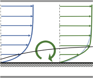
 $1/Re_\ell$ precisely represents the laminar friction experienced by a BL at the reference Reynolds number. The rationale behind this choice is to allow for a straightforward observation of how turbulence and free-stream pressure gradients increase (or decrease) the skin friction relative to the reference laminar flow, as illustrated in figure 1.
Applying torque with respect to axis  $\ell (x)$ (black solid line) to the base blue velocity profile: (a) an anticlockwise torque (e.g. turbulent enhancement or FPG) and (b) a clockwise torque (e.g. APG).

The other terms on the right-hand side of the AMI equation, (2.7), thus represent augmentation or attenuation of the skin friction coefficient relative to the baseline laminar BL and may be summarized as follows. The second term on the right-hand side of (2.7) is the turbulent torque. It represents how the turbulence (the Reynolds shear stress) redistributes mean momentum in the BL as an anticlockwise torque and reshapes the velocity profile so as to increase the skin friction, as illustrated in figure 1(a). The third term on the right-hand side of (2.7) encapsulates the effect of free-stream pressure gradient on the skin friction. In the case of an APG, this flow phenomenon acts as a clockwise torque with respect to  $\ell$, thereby reducing
 $C_f$ (figure 1b). The AMI equation thus quantifies the competition between turbulence and an APG in terms of how they alter the skin friction of an otherwise laminar ZPG BL. Alternatively, a FPG would be represented as an anticlockwise torque (figure 1a).
The fourth term on the right-hand side of the AMI equation (grouped by parentheses) arises from the integration of the first moment of the collective streamwise and mean wall-normal fluxes. This term, known as the mean flux (or total mean flux), encompasses two distinct mechanisms: (1) the streamwise growth rate of the angular momentum (relative to the laminar BL solution) and (2) the redistribution of angular momentum via the mean wall-normal velocity. The final term,  ${\mathcal {I}}^\ell$, arises from the terms neglected in applying the BL approximation (2.6), as is typically very small for attached BLs.
The baseline laminar flow could be chosen as a Blasius or Falkner–Skan solution. Given the desired interpretation of the AMI equation, it is advantageous to use the Blasius ZPG laminar BL as the reference with which to define  $\ell$. This provides a clearer interpretation of the explicit pressure-gradient term in the AMI equation by allowing it to encapsulate all pressure-gradient effects. A further choice is needed, because a particular Reynolds number definition must be chosen to match a turbulent BL to a reference laminar BL. For example, one may choose to analyse a turbulent BL relative to a Blasius BL at the same
 $Re_{\delta _1}$ (or alternatively
 $Re_{\delta _2}$). Such a choice results in
 $\ell \sim \delta _1$ (or
 $\ell \sim \delta _2$), where the coefficient of proportionality is determined using the self-similar laminar solution:
 \begin{equation} \frac{C_f}{2}=\frac{1}{Re_\ell}=\frac{0.571}{Re_{\delta_1}}=\frac{0.221}{Re_{\delta_2}}, \end{equation}
which leads to  $\ell = 1.75 \delta _1$ (or
 $\ell = 4.54 \delta _2$). Note that the choice of
 $\ell \sim \delta _1$ or
 $\ell \sim \delta _2$ controls the interpretation of the AMI equation by defining the similarity Reynolds number for comparing the BL with its baseline laminar case. More discussion of this choice is given in Elnahhas & Johnson (Reference Elnahhas and Johnson2022). The availability of a suitable baseline laminar solution is important to enable the analysis, but may not be a significant limitation in practice. For example, self-similar or locally self-similar solutions may be found for high-speed BLs (Williams et al. Reference Williams, Di Renzo, Moin and Urzay2021; Kianfar et al. Reference Kianfar, Di Renzo, Williams, Elnahhas and Johnson2023a).
Taking the limit  $\ell \rightarrow \infty$ in the AMI equation, (2.7), the standard momentum integral equation is obtained:
 \begin{equation} \frac{C_f}{2} = \frac{\delta_1}{U_{io}} \frac{{\rm d}U_{io}}{{\rm d}\kern0.7pt x} + \frac{1}{U_{io}^2} \frac{{\rm d}( U_{io}^2 \delta_2 )}{{\rm d}\kern0.7pt x}, \end{equation}
where the displacement and momentum thicknesses are defined, respectively, as
 \begin{equation} \delta_1 \equiv \int_0^{\infty} \left(\frac{U-\bar{u}}{U_{io}}\right) \mathrm{d}\kern0.05em y \quad {\rm and} \quad \delta_2 \equiv \int_0^{\infty} \frac{\bar{u}}{U_{io}}\left(\frac{U-\bar{u}}{U_{io}}\right) \mathrm{d}\kern0.05em y. \end{equation}
The non-equilibrium Clauser parameter,
 \begin{equation} \beta = \frac{ -\dfrac{\delta_1}{U_{io}} \dfrac{{\rm d}U_{io}}{{\rm d}\kern0.7pt x}}{\tfrac{1}{2}C_f} = \frac{\delta_1}{\tau_w} \frac{{\rm d}P}{{\rm d}\kern0.7pt x}, \end{equation}
is the ratio of the pressure gradient and skin friction terms in the momentum integral equation, which does not explicitly include the turbulent stress. The AMI equation, by contrast, contains an explicit term that quantifies the impact of the Reynolds shear stress on the skin friction. In doing so, the AMI equation incorporates the pressure gradient as a torque, capturing how it alters the distribution of velocity defect within the BL in competition or cooperation with turbulence (figure 1). This line of thought gives rise to an alternative dimensionless parameter for quantifying the relative strength of an APG, defined (analogously to the Clauser parameter) as the ratio of the pressure gradient and skin friction terms in the AMI equation:
 \begin{equation} \beta_\ell = \frac{ -\dfrac{\delta_1^\ell}{U_{io}} \dfrac{{\rm d}U_{io}}{{\rm d}\kern0.7pt x}}{\tfrac{1}{2}C_f} = \frac{\delta_1^\ell}{\tau_w} \frac{{\rm d}P}{{\rm d}\kern0.7pt x}, \end{equation}
which differs from the definition of  $\beta$ in this work by employing
 $\delta _1^\ell$ instead of
 $\delta _1$. The interpretation of
 $\beta _\ell$ may be given as the fractional contribution by the free-stream pressure gradient to the change in skin friction coefficient relative to the baseline laminar ZPG BL at matching
 $Re_\ell$.
The physical difference between  $\beta$ and
 $\beta _\ell$ stems from the linear dependence of the free-stream acceleration source/sink term with respect to the mean defect velocity in (2.5). Mathematically, this leads to a difference between the zeroth- and first-moment integrals of the pressure gradient source/sink which manifests as a difference between the standard displacement thickness,
 $\delta _1$, and a moment of displacement thickness,
 $\delta _1^\ell$. Because
 $\beta _\ell$ is based on the AMI equation, it inherits the interpretative benefits of capturing the quantitative impact of the free-stream pressure gradient on the skin friction relative to the laminar ZPG baseline. Therefore, it is of interest to investigate how this difference impacts our understanding of upstream history effects through its use of the first moment of the mean velocity profile. The results in this paper are used to compare
 $\beta _\ell$ with
 $\beta$ as a measurement of the strength of pressure gradient to study the pressure-gradient history effects on turbulent statistics.
3. Datasets and numerical techniques
We consider several high-fidelity numerical simulations of incompressible turbulent BLs with non-zero pressure gradients including BLs over flat plates, wing airfoils and a two-dimensional Gaussian bump. Each simulation provides a numerical solution for the incompressible Navier–Stokes equation:
 \begin{equation} \frac{\partial u_i}{\partial t} + u_j \frac{\partial u_i}{\partial x_j} ={-} \frac{\partial p}{\partial x_i} + \nu \nabla^2 u_i - \frac{\partial \tau_{ij}}{\partial x_j}, \quad \frac{\partial u_i}{\partial x_j} = 0, \end{equation}
where a residual stress tensor model,  $\tau _{ij}$, is used in the case of LES. The LES cases have grid resolutions only slightly coarser than those of DNS, so the effect of the stress tensor model is minimal. The flow configuration of each turbulent dataset is detailed in table 1. As discussed in § 2, the AMI equation, (2.7), is used for these BL flows in a tangential–normal coordination system, neglecting the explicit curvature effects (Appendix A). Note that the smallness of explicit curvature terms in the AMI equation does not necessarily imply that curvature plays no role in the BL physics (e.g. due to implicit changes in the other terms in the AMI equation). Therefore,
 $x$ and
 $y$ denote the wall-tangential and wall-normal directions, respectively, while
 $\xi$ and
 $\eta$ represent the free-stream and normal-to-free-stream flow directions (
 $x$ and
 $y$ axes of the Cartesian coordinate system).
Turbulent BL datasets. Three types of BLs are examined: flow over an airfoil, a Gaussian bump and a flat plate. For flat plates, including ZPG, the reference Reynolds number is computed based on the displacement thickness at the inlet,  $\delta ^o_1$. The reported values of
 $\beta$ are associated with the APG region
 $Re_{\delta _1} \leq 6500$.

3.1. Wing dataset
The datasets for the wing simulations correspond to the suction side of the NACA 4412 airfoil at an angle of attack of  $5^\circ$ (Vinuesa et al. Reference Vinuesa, Negi, Atzori, Hanifi, Henningson and Schlatter2018; Atzori et al. Reference Atzori, Vinuesa, Stroh, Gatti, Frohnapfel and Schlatter2021, Reference Atzori, Mallor, Pozuelo, Fukagata, Vinuesa and Schlatter2023). Referred to as the Wing, the Reynolds number based on the chord length,
 $c$, is
 $Re_c = U_\infty c /\nu = 400\,000$, where
 $U_\infty$ denotes the free-stream velocity. After the BL is tripped at 10 % chord, the turbulent BL experiences deceleration in the streamwise direction (APG) over the domain of interest in this paper, resulting in Clauser parameter values in the range
 $0<\beta <40$ along the chord length up to 95 % chord. Apart from the reference Wing case, two other BLs under the same flow configuration are studied, but with control schemes employing surface suction (Wing-suction) and blowing (Wing-blowing). The control surface extends from
 $\xi /c = 0.25$ to
 $\xi /c = 0.855$, with a constant control intensity set at
 $0.1\,\%$ of
 $U_\infty$. The AMI analyses of the flow control studies are shown in Appendix B.
The wing simulations conducted in this study utilize WRLES on the open-source Nek5000 solver, which uses the spectral-element method developed by Patera (Reference Patera1984). The LES filtering technique follows the approximate deconvolution relaxation term (ADM-RT) subgrid model developed by Schlatter, Stolz & Kleiser (Reference Schlatter, Stolz and Kleiser2004). Boundary conditions at the inlet, upper and lower sides are provided by a RANS simulation, while a local-stress outflow condition is utilized for the rear side of the domain (Dong, Karniadakis & Chryssostomidis Reference Dong, Karniadakis and Chryssostomidis2014). The mesh is generated based on the wall-shear stress from RANS simulations to ensure a resolution of approximately  $(\Delta \xi ^+,\Delta \eta ^+,\Delta z^+) <(18, 0.64, 11.9)$ in the turbulent region of the domain, where superscript
 $(+)$ denotes wall units (normalized by
 $\delta _\nu =\nu /u_\tau$, where
 $u_\tau =\sqrt {{\tau }_w/\rho }$ is the friction velocity) and
 $z$ represents the spanwise direction. While we refer to this as a WRLES due to the use of a subgrid-scale stress model, the grid resolution is only slightly coarser than typical DNS resolutions. Vinuesa et al. (Reference Vinuesa, Negi, Atzori, Hanifi, Henningson and Schlatter2018) reported that averages were taken over approximately
 $10$ eddy turnover times in the original simulation. A detailed analysis of statistical convergence is given in an appendix of Atzori et al. (Reference Atzori, Vinuesa, Fahland, Stroh, Gatti, Frohnapfel and Schlatter2020). The data used in this paper include additional averaging time, about twice a long as reported in the above references. For further information regarding the numerical set-up, the reader is referred to Vinuesa et al. (Reference Vinuesa, Negi, Atzori, Hanifi, Henningson and Schlatter2018) and Atzori et al. (Reference Atzori, Vinuesa, Fahland, Stroh, Gatti, Frohnapfel and Schlatter2020, Reference Atzori, Vinuesa, Stroh, Gatti, Frohnapfel and Schlatter2021, Reference Atzori, Mallor, Pozuelo, Fukagata, Vinuesa and Schlatter2023).
3.2. Bump dataset
The Bump dataset analysed in this paper comes from a DNS of a turbulent BL over a two-dimensional Gaussian bump performed by Balin & Jansen (Reference Balin and Jansen2021). The surface of the bump is defined by the equation  $\eta (\xi ) = h \exp (-(\xi /\xi _0)^2)$ in the Cartesian coordinate system. This geometry, illustrated in figure 4(a), is designed to replicate the three-dimensional bump flow (Slotnick Reference Slotnick2019) experimentally studied by Williams et al. (Reference Williams, Samuell, Sarwas, Robbins and Ferrante2020). In the bump's surface relation,
 $h=0.085L$ and
 $\xi _0=0.195L$ are length parameters describing the bump's dimensions, with
 $L=0.9144$ m representing the length of the square cross-section of the wind tunnel used in the experimental set-up. The flow is characterized by a reference Reynolds number
 $Re_L = U_\infty L/\nu = 1\,000\,000$, where the dimensional free-stream velocity
 $U_\infty = 16.4$ m s
 $^{-1}$, matching standard sea level conditions, resulting in an incompressible flow with Mach number
 $M = 0.045$. This flow experiences an alternating pressure gradient due to surface curvature, resulting in a weak APG region upstream, followed by a strong FPG upstream of the bump's peak at
 $\xi /L = 0$. Downstream of the bump's peak, a severe APG induces incipient flow separation (
 $\beta \to \infty$).
The DNS was performed using the stabilized finite-element method by applying trilinear hexahedral elements and second-order-accurate, implicit time integration following Whiting (Reference Whiting1999) and Jansen, Whiting & Hulbert (Reference Jansen, Whiting and Hulbert2000). A no-slip, no-penetration BC is imposed at the bump's surface, while the top BC (at  $\eta /L = 0.5)$ was modelled as an inviscid wall offset by the RANS-predicted displacement thickness described above with zero transpiration (zero velocity component normal to the surface) and zero traction. The inflow is generated by a synthetic turbulence generator (Shur et al. Reference Shur, Spalart, Strelets and Travin2014). Finally, for the outflow weak enforcement of zero pressure was applied along with zero traction. The computational grid used for DNS has a typical spacing of
 $(\Delta \xi ^+,\Delta \eta ^+, \Delta z^+ ) < (15, 10, 8 )$ with the minimum
 $\Delta \eta ^+ = 0.1$ near the surface, in wall units. The reader is referred to Balin & Jansen (Reference Balin and Jansen2021) for more information about the numerical set-up. The primary concern of the simulation was of the BL flow prior to incipient separation, so the present analysis of the resulting dataset is restricted to this region of the flow. As was the case for the discussion in Balin & Jansen (Reference Balin and Jansen2021), no analysis is made in this paper of incipient separation or other downstream aspects of the flow.
3.3. Flat-plate dataset
For comparison purposes, we also investigate a series of turbulent BLs developing over a flat plate. These simulations were conducted using WRLES, employing the ADM-RT subgrid model, similar to the approach used for the airfoil simulations. The simulations were executed using the SIMSON code, a pseudo-spectral-based solver developed by Chevalier et al. (Reference Chevalier, Schlatter, Lundbladh and Henningson2007). Specifically, we examine data from the ZPG case simulated by Eitel-Amor, Örlü & Schlatter (Reference Eitel-Amor, Örlü and Schlatter2014), as well as APG cases simulated by Bobke, Örlü & Schlatter (Reference Bobke, Örlü and Schlatter2016) and Bobke et al. (Reference Bobke, Vinuesa, Örlü and Schlatter2017), both with similar numerical set-up that results in spatial resolution  $(\Delta x^+,\Delta y^+, \Delta z^+ ) = (20, 0.2-30, 10 )$ in wall units. For the flat plates with APG, the pressure gradient was imposed through the variation of the free-stream velocity at the top of the numerical domain, following the near-equilibrium definition by Townsend (Reference Townsend1976). The wall-tangential and wall-normal coordinates are aligned with the Cartesian coordinate system in these simulations, so no mapping is required.
3.4. Numerical techniques for AMI analysis
Because the AMI analysis is applied in a curvilinear coordinate system following the surface in both the Wing and Bump flows, an appropriate tensor rotation is employed to map the flow statistics from the Cartesian frame of reference to local orthogonal directions. Additionally, as detailed in § 2, we utilize the methodology developed by Griffin et al. (Reference Griffin, Fu and Moin2021) to locally reconstruct an inviscid velocity at the wall,  $U_{io}(x)$, for each streamwise position and predict the location of the BL edge based on
 $\delta _{99}$. In the Bump case, which has the strongest curvature of the cases considered, the surface-normal rays (in the
 $y$ direction) were examined at each streamwise location, confirming they intersect neither within nor near the BL.
Figures 2(a) and 2(b) illustrate the reconstructed approximation to the irrotational velocity,  $U$, as dashed lines alongside the mean velocity profiles,
 $\bar {u}$ normalized by
 $U_\infty$, at three distinct streamwise locations for Wing and Bump, respectively. As expected, there is a remarkable agreement between
 $U$ and
 $\bar {u}$ profiles within the outer flow, marked beyond the black symbols that indicate the prediction of
 $\delta _{99}$. This confirms that there is significantly non-uniform velocity in the region of the flow which satisfies the Bernoulli equation. For example, the three streamwise locations in the Bump flow are associated with the region under strong FPG
 $\xi /L = -0.12$, strong APG
 $\xi /L = 0.15$ and very close to the separation point
 $\xi /L = 0.22$, and even near the separation point, the local reconstruction method of
 $U$ and
 $\delta _{99}$ is quite reasonable. It is important to note that the trends observed in the computed
 $U_{io}$ and predicted BL edge velocity (
 $U_e$) are similar. The reconstructed irrotational velocity at the wall,
 $U_{io}$, is used throughout the rest of the paper because it was more effective at minimizing the (normalized) residual error in the AMI equation,
 \begin{equation} \epsilon(x) = \frac{|C_f - 2 {\rm RHS}|}{C_f}, \end{equation}
for both the Wing and Bump cases. Here, RHS represents the sum of all terms on the right-hand side of (2.7). Appendix A contains more specific discussion of residual errors. Note that the normalized residual error defined in (3.2) includes multiple sources of error, including both statistical convergence errors and error related to neglecting surface curvature. Errors due to neglecting terms via the standard BL assumptions,  ${\mathcal {I}}^\ell$ in (2.7), are not included in the residual error.
Example calculations of the locally reconstructed inviscid velocity,  $U$, along the wall-normal direction for (a) Wing and (b) Bump datasets. The solid lines represent the mean streamwise velocity from the simulation and the dashed lines show the inviscid velocity profiles reconstructed using the method of Griffin et al. (Reference Griffin, Fu and Moin2021). Both velocity profiles are normalized by the free-stream velocity,
 $U_\infty$. The solid black lines and symbols denote the location of (normalized)
 $\delta _{99}$.

To compute the streamwise derivatives of flow statistics required for closing the AMI budget, we utilize the second-order central finite-difference scheme, excluding the end grid points. However, it is worth noting that computing these derivatives can amplify natural turbulent noise, which tends to increase  $\epsilon$ (Elnahhas & Johnson Reference Elnahhas and Johnson2022; Kianfar et al. Reference Kianfar, Di Renzo, Williams, Elnahhas and Johnson2023a). Furthermore, for the numerical wall-normal integration in the AMI analysis, we employ the midpoint scheme.
4. Angular momentum integral analysis
This section includes the results and discussion pertaining to the AMI-based analysis of the DNS and WRLES datasets. First, the Wing and Bump datasets are independently analysed and discussed in §§ 4.1 and 4.2, respectively. Then, those datasets are compared with the flat-plate BLs in § 4.4, with particular attention to the impact of upstream history on the BL profiles and skin friction.
4.1. Flow over airfoil
In this section, we employ the AMI equation to analyse a turbulent BL over the suction side of a NACA 4412 airfoil at an angle of attack of  $5^{\circ }$, referred to as the Wing case in table 1. The objective is to quantitatively study the interaction of turbulence and the APG in terms of ‘torques’ which compete to reshape the mean velocity profile and alter the skin friction relative to a baseline laminar solution.
Figure 3 presents the non-negligible terms of the AMI equation, (2.7), for the Wing case. The budget includes the four major terms in the AMI equation, namely laminar friction, turbulent torque, pressure gradient and mean flux. Following previous work (Elnahhas & Johnson Reference Elnahhas and Johnson2022; Kianfar et al. Reference Kianfar, Di Renzo, Williams, Elnahhas and Johnson2023a,Reference Kianfar, Elnahhas and Johnsonb), the momentum thickness is used to define the similarity Reynolds number,  $Re_\ell$, where
 $\ell =4.54 \delta _2$, a value derived from the Blasius solution. The laminar friction term thus represents the skin friction coefficient of an equivalent Blasius BL with matching momentum thickness Reynolds number,
 $Re_{\delta _2}$. The other three terms represent how each effect (turbulent mixing, free-stream pressure gradient, changes in mean streamwise growth) enhances or diminishes the skin friction coefficient relative to the Blasius BL. Figure 3(a) shows the absolute contributions of each term and figure 3(b) exhibits the relative contributions (normalized by
 $C_f/2$). The unsteady effects and terms neglected by the BL approximation, referred to as negligible terms, are not included here. This omission is justified by their limited contribution to the skin friction coefficient away from separation, as shown in Appendix A. The streamwise-averaged residual error,
 $\epsilon$, is less than
 $6\,\%$. A similar level of residual error in the AMI equations was observed in ZPG transitional and turbulent incompressible BLs (
 $\approx$2 %) (Elnahhas & Johnson Reference Elnahhas and Johnson2022; Kianfar et al. Reference Kianfar, Elnahhas and Johnson2023b), as well as in high-speed ZPG turbulent BLs (
 $\approx$5 %) (Kianfar et al. Reference Kianfar, Di Renzo, Williams, Elnahhas and Johnson2023a). In all these cases, the residual error exhibits an oscillatory behaviour and the primary source of error was the computation of streamwise derivatives,
 $\partial (\cdot ) / \partial x$, which amplifies inherent statistical noise due to averaging over a finite amount of data. That is, the residual error could be further reduced with additional averaging in time. In addition, the small residual error validates our assumption on neglecting the geometrical curvature effects.
The AMI budget with respect to the chord length,  $\xi /c$, for the Wing case (table 1): (a) the absolute budget and (b) the relative budget normalized by
 $C_f/2$. In (b), for scaling purposes, the black line denotes 100 % contribution to
 $C_f/2$. In (a,b) the faded black dotted line represents the residual of the AMI equation.

Compared with ZPG turbulent BLs, APG turbulent BLs exhibit a faster reduction of skin friction coefficient as the flow develops downstream, shown with a black line in figure 3(a). The BL is fully turbulent and its skin friction coefficient significantly exceeds that of the equivalent laminar BL. In fact the relative contribution of the laminar friction to the AMI equation is small throughout the domain of interest. In contrast, the turbulence-induced enhancement of surface friction by the turbulent torque in the AMI equation is substantial. Consistent with previous ZPG results (Elnahhas & Johnson Reference Elnahhas and Johnson2022), its relative contribution to the skin friction is near  $100\,\%$ within the range of
 $0.2<\xi /c<0.4$, where
 $\beta < 2$ (weak-to-moderate pressure gradient). Interestingly, the streamwise variation of the turbulent torque is relatively small, varying by approximately 13 % from
 $\xi /c=0.2$ to
 $\xi /c=0.9$, even under strong downstream APG.
As expected, the pressure-gradient torque is negative, acting to decrease the skin friction, and strengthens rapidly as the flow approaches the trailing edge. The normalized contribution of the pressure gradient shown in figure 3(b) exhibits a range from approximately  $0\,\%$ upstream to more than
 $-$600 % (
 $\beta _\ell = 6$), highlighting the profound impact of pressure gradient on the transport of momentum deficit and, consequently, wall-shear stress. Note that the relative contribution of the pressure gradient to the attenuation of the skin friction coefficient is equal to the AMI-based modified Clauser parameter,
 $\beta _\ell$ in (2.15). As the non-equilibrium caused by pressure gradient ramps up downstream, the mean flux term in the AMI equation opposes the pressure-gradient effects. The friction enhancement by the mean flux becomes significant for
 $\beta > 2$, where the impact of pressure gradient is two times greater than that of wall shear stress. While the mean flux negatively contributes to
 $C_f/2$ with little downstream variation in turbulent ZPG BLs (Elnahhas & Johnson Reference Elnahhas and Johnson2022; Kianfar et al. Reference Kianfar, Elnahhas and Johnson2023b), here in APG BLs, it increases and partially offsets the growing negative contribution of pressure gradient.
In addition to the baseline Wing case studied in detail here, two flow control cases are studied in Appendix B applying blowing and suction at the airfoil surface. The further application of the AMI equation to analyse the effectiveness of flow control schemes is deferred to future studies.
4.2. Flow over Gaussian bump
This section examines an incompressible fully turbulent BL over a two-dimensional Gaussian bump, referred to as Bump flow in table 1 (Balin & Jansen Reference Balin and Jansen2021). This presents a more complex scenario due to the alternate APG and FPG induced by the bump's surface curvature. Specifically, the BL experiences a significant FPG from  $\xi / L = -0.29$ to the peak of the bump at
 $\xi / L = 0$, followed by an extreme APG downstream, leading to BL separation where
 ${\tau }_w \leq 0$. The Bump flow thus provides an interesting comparison with and contrast to the Wing flow analysed in § 4.1.
Within the streamwise range of interest in this paper, the averaged residual error ( $\epsilon$) is maintained at
 $\epsilon < 10\,\%$ (equation (3.2)). Downstream of the bump's peak, characterized by an APG (
 $\xi /L\leq 0.18$), the averaged
 $\epsilon$ further diminishes to approximately
 $6\,\%$, followed by a noticeable escalation approaching the incipient separation region (which is therefore not analysed in this paper). There are multiple potential reasons for the observed trends in residual error. In our experience, the level of residual error is most sensitive to averaging time (statistical convergence). The residual error upstream of the incipient separation is acceptable for the present analysis, but could possibly be reduced with longer time averages, especially in this case due to the natural unsteadiness of the separation bubble. A brief analysis of the full AMI budget and BL assumptions is reported in Appendix A. Wei, Li & Wang (Reference Wei, Li and Wang2024) investigated the role of terms neglected by the BL assumption for the momentum integral equation, and future work can explore similar considerations for the AMI equation for separated flows.
Figure 4 presents the main terms in the AMI equation (2.7) for the Bump flow. To aid the interpretation of the AMI analysis, figure 4(a) illustrates the alternating APG and FPG due to the geometry of the surface. The BL first encounters weak APG as it approaches the bump, followed by relatively strong FPG on the upstream side of the bump. For  $0 \leq \xi /c \leq 0.4$, the BL experiences strong APG, leading to flow separation at
 $\sim \xi /c=0.2$ (where the black line in figure 4(b),
 $C_f/2$, becomes weakly negative). All four primary terms in the AMI equation are shown in figure 4(b): laminar friction, turbulent torque, pressure gradient and mean flux. As in the case of the Wing analysis, the AMI equation is calculated relative to a laminar BL with matching
 $Re_{\delta _2}$, using
 $\ell = 4.54 \delta _2$ (derived from the Blasius solution). The contributions of unsteady effects and terms neglected by BL approximations – referred to as negligible terms – are minimal upstream of the separation point. Therefore, we do not exhibit these flow phenomena in the main paper, but they are recorded in Appendix A. Figure 4(c) focuses on the turbulent torque and splits the associated integral into contributions from different regions of the turbulent BL.
The AMI analysis for the BL over a Gaussian bump simulated by Balin & Jansen (Reference Balin and Jansen2021): (a) the geometry of the bump in the normalized ( $\xi$–
 $\eta$) plane, (b) the AMI budget with respect to
 $\xi /L$ and (c) the contribution to turbulent torque confined within the inner layer (
 $\kern0.7pt y/\delta _{99} \leq 0.1$), log-law region (
 $\kern0.7pt y/\delta _{\nu } \geq 30$ and
 $y/\delta _{99} \leq 0.3$) and outer layer (
 $\kern0.7pt y/\delta _{\nu } \geq 50$) with respect to
 $\xi /L$. In (a), the dotted and solid black lines represent
 $\ell$ and
 $\delta _{99}$, respectively. In (b), the faded black dotted line denotes the residual error in the AMI equation. Moreover, asterisk symbols represent the three streamwise locations at which turbulent statistics are compared in figure 5. In (c), the full turbulent torque is provided with faded colour for the sake of comparison.

According to figure 4(b), within the FPG region on the upstream half of the bump starting at  $\xi / L = -0.29$, the skin friction coefficient initially increases, reaching a peak at
 $\xi /L=-0.14$. According to the AMI budget, this enhancement is primarily attributed to the simultaneous increase of the turbulent torque and the pressure gradient, only partially offset by the mean flux. As the flow approaches the peak of the bump, the FPG term decreases rapidly. Balin & Jansen (Reference Balin and Jansen2021) presented compelling evidence that the BL in this dataset undergoes relaminarization with onset near
 $\xi / L = -0.15$. The turbulent torque increases through the early FPG region, reaches a maximum around
 $\xi /L = -0.2$ and decreases through the (incomplete) relaminarization region up to the top of the bump at
 $\xi /L = 0$.
Figure 4(c) defines three partial contributions to the turbulent torque as integrals of the Reynolds shear stress over (i) the inner layer defined as  $y^* = y/\delta _{99} < 0.1$, (ii) the outer layer defined as
 $y^+ > 50$ based on local friction units and (iii) the log-law (overlap) layer defined as
 $y^+ > 30$ and
 $y^* < 0.3$ representing the region where the mean velocity profile is approximately logarithmic with wall-normal distance for an equilibrium wall-bounded flow. These definitions are based on Pope (Reference Pope2000). Note that the mean velocity profile departs significantly from the standard logarithmic law over most of the bump's surface (Balin & Jansen Reference Balin and Jansen2021). As defined, these three layers overlap, so the sum of the turbulent torques from each of the three is not equal to the total turbulent torque.
As is true for ZPG BLs, the outer layer is responsible for the overwhelming majority of the turbulent skin friction enhancement. The primary reason for this is that the outer layer encompasses the majority of the domain and the Reynolds shear stress integral in the AMI equation is unweighted. From the AMI perspective (comparing turbulent BLs with equivalent laminar BLs), the fluctuations in the outer layer are more influential in the sense that they transport momentum over larger distances in the wall-normal direction. Thus, it is particularly noteworthy that the inner-layer contribution to the turbulent torque remains relatively constant in the FPG region and becomes significant in the APG region upstream of incipient separation. This corresponds to the initiation and growth of an internal layer in the FPG region upstream of the apex as the turbulence in the outer layer decays. Then, the retransition process initiates relatively close to the wall. These features may be seen in the Reynolds stress profiles and visualizations in Balin & Jansen (Reference Balin and Jansen2021). Figure 4(b) shows that the significant decline in turbulent torque in the strong FPG region is accompanied by a corresponding increase in the laminar friction from  $10\,\%$ to about
 $17\,\%$ of the local skin friction coefficient.
Just upstream of the bump's peak, while the flow is still experiencing FPG and relaminarization, pressure gradient and mean flux become smaller in magnitude and reach a plateau. However, this equilibrium is disrupted immediately downstream of the peak as the flow begins to encounter an APG. Following the upstream relaminarization, a sort of retransition to turbulence occurs. As the strength of the APG increases, the turbulent torque also increases leading to a short-lived rise in the skin friction coefficient. This phenomenon is reminiscent of transition to turbulence. However, the AMI equation reveals important differences between this APG phenomenon and the transition of a laminar BL to a turbulent one. For example, in prior studies of transitional ZPG BLs (Elnahhas & Johnson Reference Elnahhas and Johnson2022; Kianfar et al. Reference Kianfar, Elnahhas and Johnson2023b), the growth in the turbulent torque significantly outpaced the growth in skin friction, with partial offset coming from the mean flux term. Under the influence of APG, however, the mean flux does not resist the growth in the turbulent torque. On the other hand, it significantly contributes to increasing  $C_f$ to counteract the substantial APG.
Furthermore, examining figure 4(c), it is evident that the initial boost in turbulent torque is not confined solely to the outer layer; the inner layer's Reynolds shear stress also experiences a significant increase. Notably, during the retransition, the increase in turbulent torque of the outer layer lags the increase closer to the wall, reflecting the growth of an internal layer in the APG region (Balin & Jansen Reference Balin and Jansen2021). As a result, the outer layer does not contain the dominant share of the turbulent torque, confirming that the skin friction enhancement through retransition is driven first by near-wall turbulence and later by turbulence further from the surface once the internal layer penetrates into the outer region of the BL. Thus, the AMI equation provides a quantitative assessment of the flow physics observed by Balin & Jansen (Reference Balin and Jansen2021) and others in terms of the skin friction coefficient.
Interesting similarities and differences between the turbulent APG BLs in the Bump (figure 4) and Wing (figure 3) cases may be observed. Both flows show the rapid growth of the opposing pressure-gradient torque and the mean flux. Prior to separation, one important difference between the two flows is that the turbulent torque increases significantly over the APG region in the Bump case whereas it is nearly constant in the APG region on the suction surface in the Wing case. The increase of the turbulent torque continues and even accelerates downstream of the peak  $C_f$, driven mostly by a faster increase of Reynolds shear stress in the outer layer.
Despite the friction enhancements by both turbulent torque and mean flux, they prove insufficient, as APG forces the flow to separate at approximately  $\xi /L=0.2$ in the Bump case. The trends in the pressure gradient and mean flux terms from the AMI equation reverse, but the residual error in the AMI equation becomes too large (presumably due to statistical convergence errors) to justify further interpretation of the results without further time averaging (see Appendix A). It is essential to note that the AMI equation, obtained solely from conservation equations, does not depend on the validity of the BL approximation. Therefore, accurate results from AMI can be expected with sufficient (time) averaging, even for separated flows. In proximity of the separated flow region, where
 $C_f \leq 0$, statistics are noisy due to an unsteady separation bubble (e.g. characterized by several frequencies (Simpson Reference Simpson1989; Na & Moin Reference Na and Moin1998)), and the BL approximations are naturally invalidated. Within that region, the amplitude of the residual error in the AMI equation increases in magnitude, shown as a faded dotted black line in figure 4(b). Even so, the effect of residual error remains significantly smaller than the turbulent torque and the pressure gradient which play the dominant role for such flows. Note that, in figure 4(c), the turbulent torque within the logarithmic region and the outer layer are omitted in the separated flow region, because the definition of
 $y^+$ is much less meaningful when
 ${\tau }_w \approx 0$.
4.3. Favourable pressure gradients: relaminarization
The relaminarization of the Bump dataset was described in Balin & Jansen (Reference Balin and Jansen2021) and in a similar simulation was analysed by Uzun & Malik (Reference Uzun and Malik2022). Here, we revisit and expound on their insights in connection with the AMI equation, mainly the behaviour of the turbulent torque (integral of the Reynolds shear stress) through the FPG region. The absolute and outer-scaled profiles of Reynolds shear stress and turbulent kinetic energy,  $k = \frac {1}{2} (\overline {u^\prime u^\prime }+\overline {v^\prime v^\prime }+\overline {w^\prime w^\prime } )$, are presented in figure 5. These profiles are plotted at three distinct streamwise locations:
 $\xi /L=-0.2$,
 $\xi /L=-0.14$ and
 $\xi /L=-0.01$; these locations are depicted in figure 4 with asterisk symbols. As shown in figure 5(a),
 $-\overline {u^\prime v^\prime }$ has the largest values at
 $\xi /L=-0.2$, where the turbulent torque peaks. However, as the FPG acts on the BL, the peak Reynolds shear stress is shifted towards the surface. This is consistent with the observations of FPG trends in figure 4(c) and with the growth of an internal layer initiated at the start of the strong FPG region (Balin & Jansen Reference Balin and Jansen2021).
Reynolds shear stress and turbulent kinetic energy profiles in the bump flow with respect to  $y^+$: absolute (a,c) and outer-scaled (normalized by
 $U_{io}^2$) (b,d). In (c,d), the dashed and dotted lines are associated with
 $\overline {u^\prime u^\prime }/2$ and
 $(\overline {v^\prime v^\prime }+\overline {w^\prime w^\prime })/2$, respectively. The streamwise location for each of the profiles is indicated by asterisks with corresponding colour in figure 4.

The turbulent torque in the AMI equation is normalized by  $U_{io}$, so figure 5(b) represents the integrand of the turbulent torque. As such it represents how the turbulent enhancement of skin friction coefficient (relative to the baseline laminar case) is distributed in the wall-normal direction. In particular, it shows how the contribution of the Reynolds shear stress to the skin friction coefficient changes through the FPG region, decreasing most severely in the outer region. The fact that the outer layer accounts for the large majority of turbulent torque skin friction enhancement in the FPG region (figure 4) helps explain the significant drop in the overall turbulent torque despite the fact that the Reynolds shear stress in the inner layer remains relatively constant in an absolute sense (figure 5a).
The Reynolds shear stress responsible for skin friction enhancement in the AMI equation requires (correlated) fluctuations in both streamwise and wall-normal velocities. The streamwise kinetic energy is produced/sustained directly proportional to the produced mean shear and the existing Reynolds shear stress. The wall-normal kinetic energy, however, relies mostly on pressure redistribution for sustenance. Interestingly, the peak turbulent kinetic energy shown in figure 5(c) increases through the FPG region, reaching a maximum near the bump's peak where the turbulent torque is minimum. This peak occurs in the buffer layer and is almost entirely due to the streamwise component (shown as a dashed line in figure 5). Kinetic energy further from the surface decreases, however. The wall-normal and spanwise kinetic energy components uniformly decrease through the FPG region (shown as a dotted line in figure 5). When normalized by  $U_{io}$ (figure 5d), the kinetic energy decreases through the FPG region, though not as severely as the Reynolds shear stress (figure 5b). This shows that the mean flow acceleration outpaces the growth in streamwise kinetic energy, while the other two components decay.
The following picture emerges (see also Uzun & Malik Reference Uzun and Malik2022). As the mean shear moves towards the surface under the action of the FPG, the production of the streamwise component of kinetic energy occurs more in the buffer layer, where the wall-blocking effect strongly suppresses the pressure redistribution of kinetic energy to the wall-normal component and the turbulence is predominantly single-component. Therefore the outer layer relaminarizes while the inner layer actually gains kinetic energy due to the increasing free-stream velocity (increasing total shear). Overall, the shifting of kinetic energy towards the surface affects a deactivation of turbulence or frozen turbulence as described by Narasimha & Sreenivasan (Reference Narasimha and Sreenivasan1973). That is, thinking in terms of integrals of the Reynolds stress components across the BL, the turbulence becomes one-dimensional so that the existing streamwise kinetic energy affects little momentum transport and the turbulent enhancement of skin friction.
The preceding two paragraphs largely summarize and synthesize insights from Balin & Jansen (Reference Balin and Jansen2021) and Uzun & Malik (Reference Uzun and Malik2022). What the AMI equation adds to this picture is an exact quantification of how the suppression of Reynolds stresses impacts the skin friction coefficient. The turbulent torque is an unweighted integral of the Reynolds shear stress across the BL and the outer layer encompassing a significant majority of the domain of integration experiences a severe attenuation of Reynolds shear stress. The Reynolds shear stress in the inner layer makes up a small portion of the turbulent torque at the beginning of the FPG region (as is typical of BLs in near-ZPG conditions). Therefore, even though the Reynolds shear stress maintains a near-constant magnitude in the near-wall region, the overall turbulent torque decreases dramatically, especially through relaminarization. The RANS models typically over-predict the skin friction coefficient in relaminarizing BLs and the AMI analysis of RANS results could help evaluate the relative importance of model errors related to RANS predictions of Reynolds stress profiles through the FPG region.
4.4. Adverse pressure gradient: AMI budget
Next, the focus turns to the effect of APG on turbulent BLs. In particular, it is fruitful to compare and contrast the AMI budget and statistics of the APG region of the Wing and Bump cases with a set of flat plates that experience weak-to-moderate APG, as detailed in the dataset provided in table 1. In the APG region, the reference Blasius BL is set based on matching the Reynolds number based on the displacement thickness,  $Re_{\delta _1}$, by setting
 $\ell =1.75 \delta _1$ based on (2.11). The choice of the Blasius BL allows for clean isolation of pressure-gradient effects in a single term of the AMI equation, in contrast to choosing a Falkner–Skan BL with some APG effects baked into the laminar skin friction. The displacement thickness is selected for the AMI length scale for APG analysis,
 $\ell \sim \delta _1$, because of its significance in the pressure-gradient term in the momentum integral equation and the definition of non-equilibrium Clauser parameter, (2.12) and (2.14).
Based on the available data from the Wing and Bump datasets, the current investigation shows results for streamwise positions corresponding to  $1400 \leq Re_{\delta _1} \leq 6500$, where
 $Re_{\delta _1} = U_{io} \delta _1/\nu$, and to regions where
 $0\leq \beta < 40$ and
 $0\leq \beta _\ell < 20$. For the Bump dataset, it is useful to relate this range of
 $Re_{\delta _1}$ to a few key landmarks. First, the apex of the bump occurs at
 $\xi /L = 0.00$ where
 $Re_{\delta _1} \approx 1360$. The small local maximum in skin friction caused by retransition occurs at
 $\xi /L \approx 0.05$ where
 $Re_{\delta _1} \approx 1850$. The analysis by Balin & Jansen (Reference Balin and Jansen2021) includes up to
 $\xi /L = 0.1$ where
 $Re_{\delta _1} \approx 3300$. Here we consider up to
 $\xi /L \approx 0.145$ (
 $Re_{\delta _1} = 6500$). We end our analysis upstream of incipient separation (
 $\xi /L \approx 0.19$,
 $Re_{\delta _1} \approx 11\,000$). The detailed physics of retransition can be sensitive to grid resolution (Shur et al. Reference Shur, Spalart, Strelets and Travin2021), given the role of smaller-scale flow structures in re-establishing a fully turbulent BL. Our analysis based on the AMI equation does not include statistics of higher order than the wall-normal integral of the Reynolds shear stress. It is instructive to explore the physical response of turbulent APG BLs to different upstream histories using to the AMI equation, even if the quantitative details of the retransition history in the Bump simulation could be sensitive to grid resolution.
The primary components of the AMI equation are illustrated in figure 6 for each dataset using the associated colours given in table 1. Notably, the laminar friction in figure 6(a) is the same across all cases due to the choice of  $\ell$ based on the Blasius solution at a matched
 $Re_{\delta _1}$. This gives a unified baseline laminar BL with which all APG turbulent BL datasets are compared in the AMI analysis. As may be expected, the magnitude of the laminar skin friction is fairly small compared with the other terms in the AMI equation.
The AMI budget within the APG region with respect to  $Re_{\delta _1}$. Contribution of the substantial flow phenomena impacting
 $C_f/2$: (a) laminar friction, (b) turbulent torque, (c) torque due to pressure gradient and (d) torque due to total mean flux. (e) The contribution to
 $C_f/2$ by the sum of (c) and (d).

In contrast, the turbulent torque is a dominant contribution to the skin friction throughout the APG region (figure 6b). For each of the flat plates, the streamwise variation of the turbulent torque is quite limited, with the highest variation at only  $8\,\%$, associated with case m18. This is not surprising, given that the BLs in these cases experience relatively constant values of the Clauser parameter. More notably, the turbulent torques of the different flat-plate cases largely collapse on top of each other. For instance, the difference in the turbulent torque between cases
 $\beta 1$ and m18 never exceeds
 $7\,\%$, despite rather significant differences in the Clauser parameter (table 1). Meanwhile, the turbulent torque for the Wing BL also exhibits a low amount of streamwise variation, only
 $13\,\%$ over the investigated region, despite the Clauser parameter ranging from
 $\beta \approx 0$ to
 $\beta \approx 40$. The turbulent torque, however, shows more variation in the Bump case. As the effects of relaminarization are reversed, the early APG region, the turbulent torque experiences a substantial increase of about
 $63\,\%$ in the range
 $1400 \leq Re_{\delta _1} < 2000$. A similar rapid growth of the turbulent torque occurs during transition to turbulence (Kianfar et al. Reference Kianfar, Elnahhas and Johnson2023b). Following this retransition in the Bump case, the turbulent torque changes relatively slowly, increasing only by
 $20\,\%$ from
 $Re_{\delta _1} = 2000$ to
 $Re_{\delta _1} = 6500$. Together with figure 7(a), these observations suggest that the turbulent torque does not depend strongly on the strength of the APG, but is more sensitive to other details of the flow configuration such as an upstream history of relaminarization.
The Clauser parameter with respect to  $Re_{\delta _1}$ (a) based on
 $\delta _1$ (the classic definition) and (b) based on
 $\delta ^\ell _1$ obtained from the AMI analysis. The black dots denote the matching locations at which turbulent statistics are compared according to table 2.

Figure 6(c) shows that the pressure-gradient torques in the AMI equation are generally negative because the APG acts to attenuate the skin friction coefficient. One notable exception in the present results is the positive torque of the APG ( $\beta > 0$) in the range
 $1400 \leq Re_{\delta _1} < 2500$ for the Bump case. Mathematically, this reflects that
 $\delta _{1}^{\ell }$ becomes negative in this region. Physically, it suggests that the comparison with a laminar BL at the same
 $Re_{\delta _1}$ captures the historical influence of FPG in some way. Based on our current analysis, it is not clear whether or not this is related to relaminarization. For the flat-plate cases, there is little streamwise variation of the pressure-gradient torque, as may be expected. Further downstream in the Bump case, as also in the Wing case, the skin friction attenuation of the pressure-gradient torque grows in magnitude, competing with and eventually overtaking the magnitude of the turbulent enhancement in figure 6(b). The battle between the turbulent torque and APG torque (see figure 1) lies at the heart of the dynamics leading to BL separation, and figure 6(b,c) illustrates the ability of the AMI equation to produce a simple quantitative account of this competition.
The mean flux term in the AMI equation, figure 6(d), encapsulates the effect of mean wall-normal velocity and streamwise BL growth on the skin friction coefficient. This term often opposes (and partially cancels) the prevailing trends from other terms in the AMI equation, such as the growth of the turbulent torque during transition to turbulence. In ZPG turbulent BLs, the mean flux attenuates the skin friction by absorbing some of the turbulent torque into an increase of the BL's moment of momentum by increasing the physical thickness of the BL. In the flat-plate APG cases, the mean flux term is also negative, in opposition to the turbulent torque, which is stronger than the pressure gradient torque. The mean flux varies little in the streamwise direction for these cases, following the trend in the pressure-gradient and turbulent torques. In the Wing and Bump cases, the mean flux follows the inverse trend of the pressure-gradient torque and undergoes a sign change near the location where the pressure-gradient torque overtakes the turbulent torque in magnitude. This signals that the mean flux transitions into a regime primarily characterized by absorption of the pressure-gradient torque into streamwise changes in the moment of momentum as well as a growth in the mean wall-normal velocity. Finally, as turbulence is restored after relaminarization between  $Re_{\delta _1}=1400$ and
 $Re_{\delta _1}=2000$ in the Bump case, the mean flux generates an increasingly negative contribution to resist the growing turbulent torque. A similar observation has been made for ZPG transitional BLs (Elnahhas & Johnson Reference Elnahhas and Johnson2022; Kianfar et al. Reference Kianfar, Elnahhas and Johnson2023b).
Given the opposite trends of pressure gradient and mean flux in figure 6(c,d), the summation of these two terms is explored in figure 6(e). In each BL case, this combination reaches an approximately streamwise-constant value (for  $\ell = 1.75 \delta _1$) even for the Wing and Bump BLs undergoing strong streamwise development forced by a strong APG. This suggests a picture in which, in addition to the momentum transport of turbulence, the pressure-gradient torque must also generate significant mean wall-normal velocity and streamwise BL growth to force the BL to separate.
4.5. Adverse pressure gradients: AMI-based Clauser-like parameter
The commonly used Clauser parameter, (2.14), emerges from the momentum integral equation, (2.12), as the ratio of the pressure-gradient term and the skin friction coefficient. Similarly, the ratio of the pressure-gradient torque in the AMI equation, figure 6(c), and the skin friction coefficient leads to a new AMI-based Clauser parameter,  $\beta _\ell$. This AMI-based Clauser-like parameter physically represents the fractional attenuation of the skin friction coefficient due to the direct effect of the APG imposed by the free stream, in competition with the turbulent stress. Mathematically,
 $\beta _\ell$ provides this streamlined interpretability by careful treatment of the linear dependence of the free-stream source/sink term on the defect velocity in (2.5) in terms of the implied impact on how momentum is (re)distributed in the wall-normal direction by the imposed free-stream pressure-gradient force (see figure 1). As such, it is of interest to explore the similarities and differences relating to the use of
 $\beta$ and
 $\beta _\ell$ to characterize APG turbulent BLs.
Figure 7 illustrates the trends of  $\beta$ and
 $\beta _\ell$ over the range of
 $Re_{\delta _1}$ explored in figure 6. The overall trends of
 $\beta$ and
 $\beta _\ell$ are similar; however,
 $\beta$ spans from
 $0$ to
 $40$, and
 $\beta _\ell$ yields smaller values in the range
 $0 < \beta _\ell < 20$ because the
 $1 - y/\ell$ weighting in the integral for
 $\delta _1^\ell$ reduces it compared with
 $\delta _1$. Additionally, the growth rates of
 $\beta$ and
 $\beta _\ell$ differ, leading to different intersection (or matching) locations between the datasets. The most significant difference in behaviour between
 $\beta$ and
 $\beta _\ell$ corresponds to the Bump dataset, where the plot of
 $\beta _\ell$ versus
 $Re_{\delta _1}$ shifts to the right compared with the plot of
 $\beta$. The differences in BL characterization between
 $\beta$ and
 $\beta _\ell$ observed in figure 7 raises the question of how an analysis of history effects may be affected by taking into account the AMI equation. That is, if two BLs have the same Reynolds number and
 $\beta$ or
 $\beta _\ell$, to what degree do different upstream conditions alter the state of the BL at the matching point?
The matching location has been the subject of several studies examining the pressure gradient history effects on turbulent statistics. Specifically, Bobke et al. (Reference Bobke, Vinuesa, Örlü and Schlatter2017) chose the matching  $Re_\tau$–
 $\beta$ to examine the upstream pressure gradient history effect. Some of the differences observed in that study can be accounted for using a Reynolds number based on the displacement thickness rather than the local wall shear stress. To deepen our understanding of the similarities and differences between APG BLs having various upstream histories, including the mean streamwise velocity and Reynolds stress components, matching locations for
 $Re_{\delta _1}$–
 $\beta$ and
 $Re_{\delta _1}$–
 $\beta _\ell$ between the different APG BL datasets are explored in this subsection. All such matching points are recorded in table 2.
Matching positions between  $Re_{\delta _1}$–
 $\beta _\ell$ and
 $Re_{\delta _1}$–
 $\beta$ for the dataset in table 1.

Furthermore, figure 8 illustrates profiles of the inner-scaled mean streamwise velocity,  $\bar {u}$, and Reynolds stress components,
 $\overline {u^\prime _i u^\prime _j}$, for matching points V (Wing–m18), X (Bump–m18) and XI
 $_6$ (Wing–Bump) based on both
 $\beta _\ell$ and
 $\beta$. These corresponding locations are indicated in figure 7 with details provided in table 2. In all these plots, the
 $x$ axis represents the wall-normal position normalized by
 $\ell = 1.75 \delta _1$, while the insets present the profiles with respect to
 $y^+$. In figure 8 the bold lines depict the profiles at matching points for
 $Re_{\delta _1}$–
 $\beta _\ell$, and faded colours represent profiles from matching points for
 $Re_{\delta _1}$–
 $\beta$.
The APG history effect on inner-scaled flow statistics with respect to  $y/\ell$ at matching
 $Re_{\delta _1}$–
 $\beta _\ell$ (
 $Re_{\delta _1}$–
 $\beta$ faded lines) for (a,b) V,
 $3064$–
 $1.48$ (
 $2872$–
 $3.45$); (c,d) X,
 $3232$–
 $1.57$ (
 $1638$–
 $1.54$); and (e,f) XI
 $_6$,
 $6245$–
 $18.51$ (
 $6404$–
 $37.54$). (a,c,e) The mean velocity and (b,d,e) the Reynolds stress components, where the solid and dotted lines represent
 $\overline {u^\prime u^\prime }^+$ and
 $-\overline {u^\prime v^\prime }^+$, respectively. The insets exhibit the same profiles versus
 $y^+$. Symbol
 $\Diamond$ denotes the wall-normal position of
 $\delta _{99}$.

As a representative of the comparison of the Wing and flat-plate datasets, figure 8(a,b) shows the mean velocity and Reynolds stress profiles at matching point V using both  $\beta$ (faded lines) and
 $\beta _\ell$ (bold lines). When matching based on
 $Re_{\delta _1}$–
 $\beta _\ell$, the mean velocity profiles from the two datasets are more similar to each other than when matching
 $Re_{\delta _1}$–
 $\beta$. The increased similarity when using
 $Re_{\delta _1}$–
 $\beta _\ell$ is also evident in the Reynolds stress profile, though less complete. The streamwise variance exhibits a secondary peak in the outer layer in addition to the buffer layer peak observed near the wall. This secondary peak is strongly influenced by the pressure gradient, and its location and magnitude vary depending on the upstream pressure-gradient history (Bobke et al. Reference Bobke, Vinuesa, Örlü and Schlatter2017). The improved similarity between the profiles from the two datasets when matching based on
 $\beta _\ell$ rather than
 $\beta$ does suggest that the AMI-based analysis does alter the perceived effect of upstream history, reducing it at least in some cases. The magnitude of the peak Reynolds stress in the outer layer is smaller for the Wing case, presumably due to the fact that it has experienced a weaker pressure gradient upstream than in the case of the flat-plate BL (see figure 7). It is worthwhile to note in passing that more robust similarity of Reynolds stress profiles was observed when comparing the Wing case with flat-plate cases having weaker pressure gradients, such as the
 $\beta 1$ or m16 cases (not shown).
As shown in figure 8(c,d), the differences between the Bump and flat-plate profiles are more significant, presumably due to the larger differences in upstream history stemming from the FPG and relaminarization in the Bump case. Compared with the  $\beta _\ell$ matching location, the matching point using
 $\beta$ occurs significantly upstream, before the streamwise variance develops the secondary outer peak. The spanwise and wall-normal variances are not shown for reasons related to the readability of the figure. Therefore, the use of the AMI-based
 $\beta _\ell$ parameter has a larger effect on the comparison of the Bump and flat-plate datasets, significantly reducing the perceived history effects.
The matching location of the Wing and Bump datasets, XI $_6$, occurs further downstream at
 $Re_{\delta _1}=6242$ for
 $\beta _\ell$ and
 $Re_{\delta _1}=6404$ for
 $\beta$. The associated profiles for these locations are shown in figure 8(e,f). There, an inner peak of the streamwise variance is no longer observed. In the Wing–Bump comparison, there is not a significant difference between the matching based on
 $\beta$ or
 $\beta _\ell$. Note that the AMI-based analysis of the Wing–Bump comparison coincidentally leads to a significant region of overlap, permitting the investigation of a case when the two BLs share the same history for some distance along the surface.
To further investigate, figure 9 displays the skin friction coefficient at matching  $Re_{\delta _1}$–
 $\beta _\ell$ (and
 $Re_{\delta _1}$–
 $\beta$ with faded colour) for the intersections (table 2) between the Wing and flat plates and Bump and flat plates. The comparison of the Wing BL with flat plate cases in figure 9(a) shows that both
 $\beta$ and
 $\beta _\ell$ indicate relatively weak history effects, especially in the case of
 $\beta _\ell$ for stronger pressure gradients. In comparison, figure 9(b) shows significant differences in
 $C_f$ for the matching locations between the Bump and flat plate cases when matched based on
 $\beta$ and
 $Re_{\delta _1}$, presumably due to significant differences in upstream history. On the other hand, the history effects do not seem as severe from the AMI-based perspective. Matching based on
 $\beta _\ell$ shows a significantly lower sensitivity of
 $C_f$ to differences between the Bump and flat-plate BLs.
Skin friction coefficient at the streamwise location of matching  $Re_{\delta _1}$–
 $\beta _\ell$ (and
 $Re_{\delta _1}$–
 $\beta$ faded colour) according to table 2. A comparison between (a) Wing and flat plates and (b) Bump and flat plates.

Finally, the skin friction coefficient comparison is carried out for the Wing and Bump cases in figure 10. Figure 7 shows that there is a single matching point in  $Re_{\delta _1}$–
 $\beta$ space, whereas in plots of
 $\beta _\ell$, the Wing and Bump lines continuously overlap each other for a segment starting at
 $Re_{\delta _1} = 3712$ (
 $\beta _\ell =3.05$) until
 $Re_{\delta _1} = 6245$ (
 $\beta _\ell =18.51$). The skin friction coefficients between the two cases converge towards each other throughout the interval with overlapping
 $\beta _\ell$, such that they are virtually indistinguishable by the point that
 $\beta$ also matches. This result shows the gradual ‘forgetting’ of upstream history (in terms of its influence on
 $C_f$) by the BL over the length of surface where the two BLs experience the same
 $\beta _\ell$. Note that figure 8(e,f) shows that the mean velocity and Reynolds stress profiles still retain some differences even after this period of forgetting.
Skin friction coefficients for the Wing and Bump datasets at the streamwise location of matching  $Re_{\delta _1}$–
 $\beta _\ell$ (
 $Re_{\delta _1}$–
 $\beta$ faded colour).

5. Conclusion
In this paper, the AMI equation, first demonstrated by Elnahhas & Johnson (Reference Elnahhas and Johnson2022) for ZPG incompressible BLs, is extended and applied as an analysis tool to study turbulent BLs undergoing non-zero pressure gradient. The AMI equation is an integral conservation law for the first moment about  $y=\ell (x)$ of momentum defect, written in terms of the skin friction coefficient. The length scale
 $\ell$ about which the moment is taken to be the centre of action of the viscous force for a laminar BL sharing the same Reynolds number, such that the skin friction of an equivalent laminar BL is isolated into a single term as a function of the Reynolds number only. This choice allows the other terms in the AMI equation such as turbulence and free-stream pressure gradients to be straightforwardly interpreted in terms of how the associated flow phenomena enhance (or attenuate) the skin friction coefficient relative to the laminar baseline case. That is, the AMI equation adapts the FIK approach (Fukagata et al. Reference Fukagata, Iwamoto and Kasagi2002) (widely used for investigating fully developed internal flows) to the scientific and engineering context of BL flows with FPGs or APGs.
The AMI equation, expressed in terms of wall-tangential and wall-normal coordinates, is applied to high-fidelity numerical turbulent BL simulation datasets, including flat-plate APG BLs, flow over the suction side of a NACA 4412 airfoil and a two-dimensional Gaussian bump flow. The AMI analysis for the BL over the flat plates and airfoil displays only a minor variation of the turbulent enhancement term, while the APG term changes substantially downstream driving strong streamwise growth and wall-normal mean velocity. In the bump flow, a region of strong FPG results in a substantial reduction of turbulent torque, co-occurring with the enhancement of skin friction by the pressure gradient term in the AMI equation. These results quantify the effect of relaminarization on the skin friction coefficient in the FPG region. Downstream of the bump's peak, flow experiences a severe APG that leads to flow separation at which the error of the AMI budget increases primarily due to the lack of sufficient averaging. Within the APG region prior to incipient separation, turbulent torque increases downstream, recovering from the upstream FPG. In this region, the contribution of the inner layer to the turbulent torque becomes much larger than elsewhere as the BL experiences a retransition.
For APG BLs approaching incipient separation, the AMI analysis concisely quantifies the competition between turbulence and the pressure gradient within its streamlined interpretive framework. One implication is the emergence of a new AMI-based Clauser parameter,  $\beta _\ell$, that carries the interpretation as the fractional attenuation of skin friction due to the APG in competition with the turbulent shear stress (see figure 1). Given its clear physical meaning, the
 $\beta _\ell$ parameter provides a new window for investigating pressure-gradient history effects on the mean velocity and Reynolds stress profiles of the airfoil, bump and flat-plate flows. The profiles were plotted at the matching Reynolds number (based on displacement thickness),
 $Re_{\delta _1}$, and
 $\beta _\ell$ compared with the original Clauser parameter,
 $\beta$. The shapes of the velocity profiles between flat plate, airfoil and bump flows show differences stemming from upstream history effects. When the Wing and Bump flows are independently compared with the flat-plate APG BLs at matching
 $\beta _\ell$, the difference in skin friction coefficient is less than when matched based on
 $\beta$. This is especially true for the Bump flow. Further, a direct comparison of the Wing and Bump flows with each other reveals a significant region where
 $\beta _\ell$ overlaps. This appears to be coincidental, but fortuitously allows for the following observation. While the skin friction coefficients of the two flows are different at the beginning of the
 $\beta _\ell$ matched region, they relax towards each other as the flows progress downstream. This suggests a gradual forgetting of older upstream history.
In conclusion, the AMI equation provides a flexible and intuitive framework for the careful accounting of free-stream pressure gradients on skin friction following in the tradition of FIK analysis (Fukagata et al. Reference Fukagata, Iwamoto and Kasagi2002). While geometric curvature effects were not significant for the flows studied here, future development of the AMI equation in curvilinear coordinates would further expand its capability. While the explicit terms related to a transformation to curvilinear coordinates did not seem necessary for the flows studied here, future development of the AMI equation in curvilinear coordinates would further expand its capability. (Note that this does not imply that the effect of surface or streamline curvature on the physical flow is negligible.) Also, future AMI-based investigation of bump flows at higher Reynolds numbers where relaminarization does not occur (Prakash et al. Reference Prakash, Balin, Evans and Jansen2024) could yield more insight into pressure-gradient history effects. Other promising applications of the AMI equation include the assessment and optimization of flow control strategies in BLs. As discussed in Appendix B for the Wing case with suction and blowing, the AMI equation quantifies the effect of non-zero wall-normal velocity at the wall on the AMI interpretation of skin friction coefficient. This analysis can further examine the impact of subsurfaces, e.g. phononic structures (Hussein et al. Reference Hussein, Biringen, Bilal and Kucala2015; Kianfar & Hussein Reference Kianfar and Hussein2023b), on BL turbulence. Additionally, it is of interest to leverage the insight from the AMI equation for developing new strategies for modelling and simulation.
Acknowledgements
P.L.J. acknowledges support by the National Science Foundation under grant number 2340121. The bump dataset is from a simulation performed by R. Balin with K. Jansen. The authors thank A. Prakash for facilitating access to the Gaussian bump DNS dataset, as well as M. Atzori and R. Vinuesa for access to their NACA airfoil simulation dataset. A. Prakash is also acknowledged for helpful discussions and feedback on a draft manuscript.
Declaration of interests
The authors report no conflict of interest.
Appendix A. Full budget of the AMI equation
The form of the AMI equation derived in this paper makes use of the standard BL assumptions to neglect certain terms in the mean momentum equation. Given that the Wing and Bump datasets involve strong pressure gradients, it is worthwhile to document the full AMI equation, including the supposedly negligible terms. For example, Wei et al. (Reference Wei, Li and Wang2024) analysed DNS data from a simulation of a BL separation bubble induced by an imposed transpiration profile at the top of the domain (Coleman, Rumsey & Spalart Reference Coleman, Rumsey and Spalart2018) and demonstrated that the negligible terms in the momentum integral equation can be quite significant for strong APGs.
A.1. Wing dataset
This appendix provides the full budget of the AMI equation, including negligible terms, for the Wing dataset. Figure 11 exhibits  $C_f/2$ and the sum of the all terms on the right-hand side of (2.7), denoted as RHS, where a great match between the left- and right-hand sides of the AMI budget is evident. Unsurprisingly, negligible terms remain insignificant even downstream under relatively higher APG.
The full budget of the AMI equation for the Wing dataset. Here,  $\ell = 4.54\delta _2$ obtained from the Blasius solution. The faded lines represent the flow phenomena already shown in figure 3.

A.2. Bump dataset
This appendix presents the complete budget of the AMI equation, including negligible terms, for the Bump dataset. Figure 12 illustrates  $C_f/2$ and the sum of all terms on the right-hand side of (2.7), labelled as RHS. A good agreement is observed between the left- and right-hand sides of the AMI equation, except in regions very close to separation (or separated flow). Additionally, downstream of the separation bubble, where flow reattachment occurs, the sum of the right-hand side of (2.7) fluctuates around
 $C_f/2$. This suggests that the AMI analysis captures the physics within this region, although insufficient averaging leads to oscillations.
The full budget of the AMI equation for the Bump dataset. Here,  $\ell = 4.54\delta _2$ obtained from the Blasius solution. The faded lines represent the flow phenomena already shown in figure 4.

As expected, negligible terms remain insignificant away from the separation region. However, near and within the separation bubble, the terms neglected by the BL approximation and unsteady acceleration become significant. Furthermore, the (absolute) contribution of negligible terms slightly increases where the flow is accelerating within the FPG region. The authors attribute this marginal enhancement to an increase in the streamwise derivatives that appear in (2.6). Specifically, the streamwise derivative of  $\overline {u^\prime u^\prime }$ is higher than that for the other regions of the flow. A further exploration of the negligible terms in the AMI equation, and how they may be used to create alternative Clauser-like parameters (Wei et al. Reference Wei, Li and Wang2024), is deferred to future work.
Appendix B. The AMI analysis of blowing and suction
Another application of the AMI equation is to assess flow control schemes, such as surface suction and blowing, along with the influence of pressure gradient on skin friction. Figure 13 illustrates the budget of the AMI equation for a turbulent BL over an airfoil under suction and blowing, compared with the reference Wing discussed earlier. For both suction and blowing, the control region spans from  $\xi /c = 0.25$ to
 $\xi /c = 0.855$ with a control intensity of 0.1 % of
 $U_\infty$, reported by Atzori et al. (Reference Atzori, Mallor, Pozuelo, Fukagata, Vinuesa and Schlatter2023). This region is shaded in grey in figure 13.
The AMI budget of the reference wing compared with the suction and blowing cases with respect to  $\xi /c$ for (a) turbulent torque, (b) pressure gradient, (c) mean flux and (d) wall BC. The shaded grey region denotes the streamwise position under suction (or blowing). In (a), faded black lines exhibit
 $C_f/2$.

With surface suction (or blowing), laminar friction is marginally higher (or lower) than the reference case as BL thickness reduces (or increases) downstream; thinning of  $\delta _{99}$ is correlated with a reduction in
 $\delta _{2}$, and hence
 $\ell$. Ignoring the contribution of laminar friction, which is not effectively impacted by suction (or blowing), a major flow phenomenon is wall BC. In the AMI equation, the direct impact of suction and blowing (or any imposed wall BC) on
 $C_f/2$ is associated with wall BC. This flow phenomenon explicitly depends on the wall-normal velocity at the surface,
 $V_w$. Figure 13(a) depicts wall BC along with
 $C_f/2$ shown in faded black lines. In these plots, suction is represented by dashed lines, and the blowing case is illustrated by dotted lines. As expected, suction naturally increases the skin friction coefficient by enhancing the wall-edge velocity gradient through the reduction of the BL thickness. On the other hand, surface blowing leads to an about
 $20\,\%$ reduction of
 $C_f$ with respect to the reference case by thickening the BL. With regular no-slip and no-penetration wall BCs, wall BC is naturally as shown for the reference wing; however, this term positively (or negatively) contributes to the surface friction in the suction (or blowing) case. For instance, in the surface suction (or blowing) case, the relative contribution of wall BC reads from
 $24\,\%$ (or
 $-$35 %) at the leading edge to approximately
 $80\,\%$ (or approximately
 $-$200 %) at the trailing edge of the control region. This monotonic increase of the relative contribution downstream is merely due to the reduction of
 $C_f/2$ because
 $V_w$ is imposed to be a constant.
Despite the limited influence of suction (or blowing) on laminar friction, the control region changes the turbulence enhancement. As shown in figure 13(b), the impact of suction (or blowing) on turbulent torque is opposite and less significant compared with its impact on  $C_f$. For example, surface suction increases the skin friction coefficient, but diminishes turbulent torque. The AMI equation quantifies the maximum change of turbulent torque to be, respectively,
 $-$10 % and
 $9\,\%$ for suction and blowing. Moreover, suction (or blowing) seems to have a cumulative effect on turbulent torque; at the trailing edge of the control region, the difference between turbulent torques is negligible, yet it increases downstream. Therefore, for the suction case, the lower downstream turbulent torque shows that surface suction alleviates the impact of pressure gradient on the upstream-to-downstream variation of the turbulence enhancement; the difference of turbulent torque between
 $\xi /c=0.2$ and
 $\xi /c=0.9$ is less than
 $1\,\%$, while in the reference case, this number was reported to be
 $13\,\%$. These results suggest that surface suction must reduce the negative contribution of pressure gradient by pulling the flow towards the wall.
As presented in figure 13(c), similar to the turbulent torque analysis, the impact of surface suction (or blowing) on pressure gradient appears to be cumulative too. Within  $\xi /c \leq 0.4$, the effect of suction (or blowing) on pressure gradient is insignificant. However, the accumulated effect becomes more pronounced downstream of
 $\xi /c = 0.4$, also slightly influencing the growth rate of pressure gradient. The AMI analysis quantifies the maximum impact of surface suction on pressure gradient to be approximately
 $14\,\%$, observed at the trailing edge of the control surface, compared with the reference wing. Surface blowing has a similar but opposite effect, enhancing the strength of pressure gradient.
Due to the natural cumulative effect of suction (or blowing) on turbulent torque and pressure gradient, mean flux is the only flow phenomenon partially resisting the immediate impact of wall BC on  $C_f$. In other words, mean flux alleviates the non-equilibrium caused by both pressure gradient and wall BC. In the spatial range of
 $0.2 \leq \xi /c \leq 0.4$, where pressure gradient is relatively weaker, the absolute contribution of mean flux to
 $C_f/2$ is insignificant, approximately
 $5\,\%$. In the suction (or blowing) case, on the other hand, mean flux resists the immediate skin friction enhancement (or reduction) caused by wall BC. The immediate response of mean flux to suction (or blowing) can be understood by looking into its subterms. As described in § 2, mean flux is the sum of the streamwise growth of the BL thickness and the mean wall-normal flux, first introduced in Elnahhas & Johnson (Reference Elnahhas and Johnson2022). Suction (or blowing) only implicitly influences the streamwise growth of the BL. On the other hand, the mean wall-normal flux absorbs the immediate change of suction (or blowing). This term, demonstrated to enhance wall shear stress in fully turbulent flows (Elnahhas & Johnson Reference Elnahhas and Johnson2022; Kianfar et al. Reference Kianfar, Di Renzo, Williams, Elnahhas and Johnson2023a,Reference Kianfar, Elnahhas and Johnsonb), exhibits a weaker effect with suction but a stronger impact with blowing at the surface of the control region. This is a consequence of suction (or blowing) altering the mean wall-normal velocity profile, influencing the wall-normal transport of momentum, particularly near the surface. For example, suction induces a region with negative mean wall-normal velocity, leading to an inverse contribution of mean wall-normal flux. Therefore, mean flux compensates for approximately
 $70\,\%$ of the wall BC's friction enhancement, primarily by generating weaker (and sometimes negative) mean wall-normal flux. Interestingly, this observation parallels findings in transitional incompressible BLs (Kianfar et al. Reference Kianfar, Elnahhas and Johnson2023b), where a small region near the surface exhibited wall-normal deceleration and
 $\bar {v}\leq 0$, forcing the near-wall flow to accelerate in the streamwise direction due to the continuity constraint. The authors contend that BLs with suction and transitional flows, which are characterized by the presence of negative near-surface wall-normal velocity, have the potential to foster more robust passive control schemes. This could be achieved through the use of a porous medium or phononic subsurfaces (Hussein et al. Reference Hussein, Biringen, Bilal and Kucala2015; Kianfar & Hussein Reference Kianfar and Hussein2023a). The negative velocity near the surface is anticipated to enhance the effectiveness of such control schemes by further stimulating the control surface.
Appendix C. The AMI analysis using the Falkner–Skan BL
In the preceding section, we primarily focused on the BL regions experiencing moderate APG, where we investigated the impact of APG on the Reynolds shear stress enhancement of skin friction coefficient using the AMI analysis. Additionally, we introduced an AMI-based non-equilibrium Clauser parameter, denoted as  $\beta _\ell$, to delve into the influence of pressure gradient history effects on turbulent statistics. However, thus far, our approach has relied on an AMI length scale derived from the Blasius solution. In this appendix, we explore an alternative approach by employing the Falkner–Skan laminar solution to determine
 $\ell$.
Our objective here is to establish a relationship for  $\ell$ within the APG region, specifically within the range of
 $1400 \leq Re_{\delta _1} \leq 6500$, by aligning the Clauser parameter between the turbulent datasets listed in table 1 and the laminar Falkner–Skan solution. In essence, we determine the coefficient
 $c$ (introduced in § 2) by utilizing the Falkner–Skan solution with the precise value of
 $\beta$ at each streamwise location.
To obtain the coefficient  $\alpha _{FS}$ based on the Falkner–Skan solution, we developed an ordinary differential equation solver using the shooting method to solve the self-similar Falkner–Skan momentum equation. The similarity form, introduced by Falkneb & Skan (Reference Falkneb and Skan1931), is defined by
 $\eta = Cyx^a$, where
 $\eta$ represents the self-similar variable, consistent with a power-law edge velocity distribution given by
 $U_e(x) = Kx^m$, where
 $C$ and
 $K$ are constants to make
 $\eta$ dimensionless and
 $m = 2a+1$. The ordinary differential equation solver selects
 $\eta = y \sqrt {(m+1){U_e(x)}/{\nu x}}$, and imposes appropriate BCs, similar to the Blasius solution for a flat plate (refer to chapter 4 in White & Majdalani (Reference White and Majdalani2006)). Using the similarity solution, the skin friction coefficient and displacement thickness, respectively, are expressed as
 \begin{equation} \frac{C_f}{2} \equiv \frac{2 \tau_w}{\rho U_e^2} = \sqrt{(m+1) \frac{\nu}{U x}}\, f^{\prime \prime}(0) \end{equation}
and
 \begin{equation} \delta_1 \equiv \int_0^{\infty}\left(1-\frac{u}{U_e}\right) {{\rm d}\kern0.05em y} = \sqrt{\frac{1}{m+1}\frac{\nu x}{U_e}} \lim _{\eta \rightarrow \infty}(\eta-f), \end{equation}
where  $f$ represents the similarity function and the prime indicates differentiation with respect to
 $\eta$. Similarly, we can derive a relationship for the Clauser parameter that reads
 \begin{equation} \beta \equiv{-}\frac{1}{U_e} \frac{{\rm d} U_e}{{\rm d}\kern0.7pt x} \frac{2 \delta_1}{C_f} ={-}\frac{ m}{m+1} \left[\frac{\displaystyle\lim_{\eta \rightarrow \infty}(\eta-f)}{f^{\prime \prime}{(0)}} \right], \end{equation}
where the term enclosed by brackets is self-similar. We further relate  $\beta$ to the AMI's length scale coefficient,
 $\alpha _{FS}$, as
 \begin{equation} \beta=\frac{-m}{m+1}\left[\lim_{\eta \rightarrow \infty}(\eta-f)\right]^2 \alpha_{FS}. \end{equation}
Figure 14(a) illustrates a plot of  $\beta$ with respect to
 $m$ within the APG region (
 $m \geq 0$). Interestingly, the plot of
 $\alpha _{FS}$ with respect to
 $\beta$ in figure 14(b) demonstrates a (semi-)linear relationship between them. Therefore, one can determine the appropriate
 $\alpha _{FS}$ at each streamwise position by knowing the Clauser parameter, i.e.
 $\alpha _{FS}(x) = 1.75 + 0.822\beta (x)$.
Self-similar Falkner–Skan solution and the Clauser parameter. Relationships between  $\beta$ and
 $m$ (a) and
 $\alpha _{FS}$ and
 $\beta$ (b).

Now that we have established a relationship between  $\beta$ and
 $\ell$, we can determine
 $\ell = \alpha _{FS} \delta _1$ by knowing the
 $\beta$ values in the turbulent dataset (table 1). As a result, when we apply this
 $\ell$ to the AMI analysis, the first term on the right-hand side of the AMI equation, representing the laminar friction (
 $1/Re_\ell$), precisely yields half of the skin friction coefficient that would be expected if the flow were laminar (with the same Reynolds number) under the same
 $\beta$. This term, although for the turbulent dataset is more distinct than in figure 6(a), weakly contributes to the skin friction coefficient. The explicit turbulent enhancement in the AMI equation based on the Falkner–Skan solution, however, remains the primary contributor to
 $C_f$.
In figure 15(a), we observe a distinct trend in the behaviour of turbulent torque compared with figure 6(b), where the analysis was based on the Blasius solution. Specifically, the behaviour of turbulent torque shows an inverse relationship with the strength of the pressure gradient, i.e.  $\beta$. For flat-plate cases characterized by weak-to-moderate pressure gradients, there is a minimal variation in turbulent torque from upstream to downstream, especially beyond
 $Re_{\delta _1}=3500$, where their
 $\beta$ is flattened. In contrast, for cases exhibiting rapid growth in
 $\beta$, such as Wing and Bump, the variation in turbulent torque from upstream to downstream is more pronounced. This behaviour can be attributed to the fact that the total Reynolds shear stress remains constant downstream, as discussed in § 4.4. Consequently, as
 $\ell$ increases with
 $\beta$, turbulent torque decreases downstream, at an inverse rate.
Turbulent torque with respect to  $Re_{\delta _1}$ when
 $\ell$ is obtained from the Falkner–Skan solution. (a) The absolute contribution to
 $C_f/2$. (b) The relative contribution (normalized by
 $C_f/2$).

Despite the significant changes in turbulent torque with  $\beta$ in the Wing and Bump cases, it is noteworthy that the relative contribution (normalized by
 $C_f/2$) of turbulent torque (as shown in figure 15b) tends to flatten downstream of
 $Re_{\delta _1}=6000$. This suggests that for relatively strong APG, e.g.
 $\beta \geq 10$, the spatial rate of change of this flow phenomenon mirrors that of the skin friction coefficient.
Using the Falkner–Skan solution as the reference flow for the AMI equation allows us to derive the AMI's Clauser parameter,  $\beta _\ell$, where
 $\ell$ varies downstream as a function of
 $\beta$. Figure 16 illustrates this
 $\beta _\ell$ with respect to
 $Re_{\delta _1}$, compared with
 $\beta$ (shown with faded lines). According to the plots of the Wing and Bump cases in figure 16, far downstream where the pressure gradient is relatively strong (
 $\beta \geq 40$),
 $\beta _\ell$ and
 $\beta$ converge to each other. To understand this phenomenon, consider an asymptotic condition where
 $\beta \to \infty$: the AMI's length scale,
 $\ell \to \infty$. Consequently, as mentioned in § 2, if
 $\ell \to \infty$, the AMI equation will recover the von Kármán integral equation, i.e.
 $\beta _\ell \to \beta$. On the other hand, for
 $\beta \to 0$ (
 $\beta < 1$), the Falkner–Skan-based AMI yields analogous results as shown in figure 7(b) for
 $\beta _\ell$ based on the Blasius solution.
The Clauser parameter with respect to  $Re_{\delta _1}$ based on
 $\delta ^\ell _1$ obtained from the AMI analysis using the Falkner–Skan laminar solution. The faded lines denote
 $\beta$ as in figure 7(a).

Additionally, in the Bump case, figure 16 indicates that  $\beta _\ell$ has marginally captured the upstream FPG effect. Therefore, compared with
 $\beta$, the plot of
 $\beta _\ell$ is slightly shifted to the right. This absorption of the FPG history effect, however, is not sufficient; also, it is weaker than what we observed in figure 7(b) for
 $\beta _\ell$ based on the Blasius solution. As a result, the matching location between Bump and flat plates occurs too early upstream when
 $\beta _\ell$ is based on the Falkner–Skan solution. Consequently, the turbulent statistics at these matching locations yield less similarity compared with what we observed for
 $\beta _\ell$ obtained from the Blasius solution, like in figure 8(c,d). This weaker similarity also manifests in the correlation between
 $C_f$ and
 $\beta _\ell$, where we compute a weaker correlation when
 $\beta _\ell$ is based on the Falkner–Skan solution rather than figure 9(b).


 Open access

