Players and Preferences

There are three types of players in the model: the firms, the bureaucrats, and the government. Utility is transferable, so everyone cares equally about money.

Firm i's production function is given by f(k _it)=rk _it, where r is a productivity parameter, and k _it is firm i's capital stock at time t. There are a large (infinite) number of identical firms of measure one. This simplifies the analysis, but our results hold for any number of firms, as discussed in Firm-specific Regulation and Appendix A. There is no competition between firms (competition is allowed in an earlier working paper version). It is also possible to allow heterogeneity, for example in r, but because that would not add any insight, we keep the model symmetric. Thus, in equilibrium, k _it=k _t, the average (and aggregate) level of capital. We therefore often drop the subscript (i) denoting firm i. In fact, we also frequently drop the subscript for time, whenever this is not misleading.

Each firm faces some regulation it must overcome. If it complies with the regulation, this costs c per unit of capital. The total cost of compliance, ck _i, is proportional to k _i because the regulation constrains production, which is proportional to k _i.Footnote ⁴

If firm i does not comply, the government's utility loss is e>0 per unit of capital, where the parameter e measures the externality of noncompliance. For this reason, the government always prefers introducing regulation if there is none, so this can explain the rule's existence in the first place.Footnote ⁵ The total externality ek _i is proportional to the size of the firm or, equivalently, the size of its production: the more the firm produces, the larger is the negative externality if it is not complying.Footnote ⁶

Similarly, a bureaucrat may also prefer that the firm compliy. Specifically, we assume that a bureaucrat receives a utility loss e _B per unit of capital if a firm does not comply. The bureaucrat and the government can of course have different preferences for compliance, so we allow e _B≠ e. Moreover, the interpretation of e _B can be very different from the interpretation of e. Consider the case of environmental regulation: a bureaucrat may not care about pollution per se, but about being punished if the firm he or she is supposed to monitor does not comply. One can therefore interpret e _B as representing the expected penalty for the bureaucrat. If the actual penalty is x and the probability of being detected is θ, then e _B=θ x. The probability of being caught, θ, may vary across bureaucrats as well as time, so let θ be uniformly i.i.d. over [0,1]. Alternatively, let θ represent the individual stigma associated with being penalized for corruption, whereas x is the expected penalty. In either case, a bureaucrat faces the cost θ xk _i for bending the rules for firm i. This cost increases in k _i because it is more likely that a large firm will be investigated, or because the penalty for such a large crime is larger. There is no need for private information in the model, so we let θ be observed by the firm before it negotiates with the bureaucrat. Moreover, let c ∈ (0, x), such that some bureaucrats (and firms) are corrupt (if θ <c/x), whereas other comply (if θ >c/x).Footnote ⁷

Bribery

Instead of complying, a firm has two alternatives. First, it may bribe the bureaucrat to “bend the rules.” That is, a firm can pay a bribe B to the bureaucrat for letting the firm proceed without complying with the regulation. The size of B is negotiated between the firm and the bureaucrat. We assume that the bargaining solution is efficient (for the bureaucrat and the firm) and let β ∈ [0, 1] measure the bureaucrat's share of the bargaining surplus. This would follow, for example, by relying on the generalized Nash bargaining solution if the bureaucrat's relative bargaining power was β.Footnote ⁸

Our key assumption is that the bureaucrat cannot commit to bend the rules in the future. Future deals remains to be negotiated at a later stage. This is quite reasonable, because bending the rules does not change the status quo (i.e., the law), and a bureaucrat cannot write enforceable contracts stating that he will not monitor the firm later. This is consistent with our assumption that firms deal with different bureaucrats over time and that corruption is illegal.

Lobbying

As an alternative to bending the rules, the firms may lobby the government to change them. To be successful, the firms must spend more resources on lobbying if the government is reluctant to relax the rule. In particular, we assume that the firms can make a take-it-or-leave-it offer to the government, specifying a transfer of size L from firms to the government.Footnote ⁹ The proofs in the Appendix tolerate that the government has some bargaining power when negotiating L. After the rule is relaxed, there is no need to comply or negotiate with the bureaucrat.

Changing the rules benefits all firms, so they may share the cost of lobbying in equilibrium.Footnote ¹⁰ Realistically, the firms negotiate how to split the cost L, and we assume that each firm ends up with an equal share of the bargaining surplus. This would be implied by relying on the Nash bargaining solution, for example.Footnote ¹¹

In contrast to the case where the bureaucrat bends the rule, changing the rules affects the status quo. To simplify, we assume that if the rules are relaxed, they are relaxed forever. This is an extreme assumption, and Appendix A discusses how it can be weakened. For our results, it is sufficient to assume that changing the rules has a longer-lasting effect than bribery. Nevertheless, note that it is straightforward to endogenize this assumption: simply assume that several legislators are pivotal in changing a law, e.g., because of a supermajority requirement, or because a proposal must pass two political chambers. If one of the pivotal legislators has preferences that are aligned with the firms, then he or she will never accept to reintroduce the rule once it is relaxed.

Investment and Growth

A firm's capital stock depreciates at rate d, but it can increase its capital stock by investing I _t at cost zI _t²/2:

(1)

We normalize the time such that k ₀=0 at t=0. The discount rate, δ, is the same for all agents. Although it is convenient to refer to “period t,” we let time be continuous in the model. This simplifies some of the calculations without affecting the results. Whether time should be discrete or continuous in the model is a matter of taste, and the results would prevail if time were discrete.

In each period t, the timing of the game is as illustrated in Figure 1. After the firms have invested, they collectively decide whether to lobby the government to change the rules. If they do, their contributions are determined in a bargaining game where each firm gets an equal share of the total surplus generated by relaxing the rules. Because every firm would thus like to maximize the total surplus, they all agree on when and whether to lobby.Footnote ¹² If the firms end up not lobbying in this period, they proceed individually. Then each firm observes the type of its bureaucrat and determines whether to offer a bribe. If these negotiations fail or are never initiated, the firm complies. As already mentioned, the firm faces a new bureaucrat every period, so that this sequence repeats itself at each time t.

FIGURE 1.

Timing of the Game

Bribes and Investments

Before deciding whether to comply, a firm learns the type θ ∈ [0, 1] of the current bureaucrat. If θ <c/x, the firm and the bureaucrat can both be better off if the firm pays a bribe B ∈ (θ xk,ck) to the bureaucrat to circumvent the regulation. The size of the bribe is determined by negotiations between the firm and the bureaucrat. By assumption, the bureaucrat's surplus (B-θ xk) is β multiplied by the total surplus from bending the rule, ck-θ xk.Footnote ¹³ The bribe B is thus

(2)

The bribe B increases in k for two reasons. First, a large k implies that the firm's cost of compliance is large, and it is thus willing to pay more to circumvent the rules. Second, if k is large, the bureaucrat's cost of bending the rule is larger (because a large firm's failure to comply is more likely to be detected or it is penalized more). For both reasons, large firms pay more bribes. Furthermore, note that if θ is large, B is large because the firm must compensate the bureaucrat for the severe expected penalty he risks. B is also increasing in c, the cost of compliance, because the bureaucrat can ask for accordingly higher bribes. This is particularly important if the bureaucrat's relative bargaining power, β, is high.

Because θ is uniformly distributed on [0,1], the probability for θ x<c, implying that the firm bribes, is c/x. A firm complies with probability 1-c/x. In other words, the larger the cost of compliance, the more firms prefer to bribe instead of comply.

Proposition 1. A fraction c/x of the firms bribe and the bribe B, given by (2), increases in the capital stock (k), the cost of compliance (c), the bureaucrat's bargaining power (β), and the expected penalty for corruption (θ x).

Before it learns the bureaucrat's type, a firm's current expected profit is

(3)

The firm's expected cost of bribing or complying, b, is increasing in the unit cost of compliance (c), the bureaucrat's bargaining power (β), and the penalty if caught taking bribes (x).

When a firm invests, it takes into account how investments affect total profit, including the impact on the bribes. To solve for the equilibrium investment, consider, first, an equilibrium where bribery takes place forever. In such a steady state, each firm will at time t plan its investments in order to solve

(4)

Proposition 2. In a bribery equilibrium, investment I is decreasing in b, and thus in the cost of compliance (c), the bureaucrat's bargaining power (β), and the penalty if caught taking bribes (x):

(5)

The more capital the firm has, the higher the bribes will be. Thus, bribery leads to a typical holdup problem, because the bureaucrat cannot commit not to ask for higher bribes once the firm is larger. This discourages the firm from investing. Because the equilibrium size of the bribe increases in c, x and β, investments do the opposite. Powerful bureaucrats (β large) extract more bribes, which reduces the incentives to invest. Harsher penalties on corruption reduce growth as well, because the bureaucrats then demand higher bribes, worsening the holdup problem. If c increases, both the cost of compliance and the bribes are larger, and investments decrease for both reasons.

Lobbying and Investments

Having solved for the steady state investments above, it is easy to calculate a firm's present discounted value, V(k _it,b), which depends on its current level of capital and the firm's expected loss due to compliance or bribery, b. If successful lobbying has taken place and the rules have been relaxed, it is no longer necessary to pay bribes. Then, the firm's investment decision is similar to (5) if just b is replaced by zero. Whether the firms benefit from lobbying thus depends on a consideration of V(k _it,b), V(k _it,0) and the cost of lobbying, L.

The total cost of lobbying, L, must be large enough to compensate the government for its utility loss from relaxing the rule. If the rule stays in place, the government's present discounted utility is V _g(k _t) =-e∫_t^∞k _b,τ(c/x) dτ, where c/x is the fraction of firms that do not comply, whereas k _b,τ is the equilibrium level of k at time τ, given that the rule stays in place. Once the rule is relaxed, and no firm needs to comply, the government's present discounted utility is V _g(k _t) =-e∫_t^∞k _l,τdτ, where k _l,τ is the equilibrium level of k at time τ, given the larger investments following liberalization. The cost of lobbying is the difference in these payoffs:

(6)

(7)

Thus, L is the government's loss, for the entire future, when relaxing the rule. As shown on the r.h.s. of (6), this loss depends not only on the current capital level, but also on the long-run steady state levels for k. This steady state level is given by k _l,∞ if the rule is relaxed, and otherwise by k _b,∞. In each case, the steady state capital level is independent of the current level, and thus the steady state utility loss for the government is independent of the current k. L therefore has a fixed component, the second term in (7), in addition to the first term, which is increasing in k.

Proposition 3. i. At equilibrium, the total cost of lobbying is given by (7).

ii. Firm i's individual cost of lobbying increases in k_i and is given by

(8)

Whereas the intuition for part (i) is explained above, part (ii) can be explained as follows: First, when negotiating the L _is, the sum must equal L, so that ∫_iL _idi=L. Second, by assumption, or by using the Nash bargaining solution, every firm gets the same share of the bargaining surplus. If the negotiations fail, the default is to bribe or comply. Thus, i's net surplus, which is V(k _it,0)-V(k _it,b)-L _i, must be the same for every firm. Because V(k _it,0)-V(k _it,b) increases in k _it, so must L _i. Intuitively, i's bribes are larger if i's level of capital, k _it, is large, as Proposition 1 shows. It is then highly important for i to circumvent the bureaucrat's power and relax the rules. The other firms can hold up i, then, and require i to contribute more to the cost of lobbying.Footnote ¹⁴

Thus, lobbying generates a holdup problem, just like bribery. In fact, investment levels turn out to be the same at any time t<T, when lobbying is coming up in the future, as they would be if bribery were to continue forever. The explanation is as follows: Remember that i's net surplus, V(k _it,0)-V(k _it,b)-L _i, must be the same for all firms, say ϖ. Thus, i's payoff is V(k _it,0)-L _i=V(k _it,b)+ϖ, and each firm is therefore ending up with its default payoff V(k _it,b), plus a constant that is independent of k _it.Footnote ¹⁵ When investing, therefore, firm i invests in such a way as to maximize its default payoff V(k _it,b), just as in the case where bribery continued forever.

If lobbying has taken place, on the other hand, there is no need to comply or bribe and the firms choose to invest more (as if b=0 in (5)).

Proposition 4. Suppose that, in equilibrium, lobbying replaces bribery at time T.

1. i. At any time t<T, each firm invests according to (5).

2. ii. At any time t>T, investments are higher and given by

   

From Bribery to Lobbying

Having derived the costs of bribery and lobbying, and the investment levels for each situation, we can compare them to determine what firms prefer to do. When bargaining over whether to lobby, each firm receives a fraction of the total surplus from relaxing the rules, and every firm prefers to maximize this total surplus. They thus agree on whether and when to lobby rather than bribe.

When k is small, the bribe is small and it is not worthwhile to pay the high cost of lobbying. However, the cost of the bribes increases faster in k than does the cost of lobbying if the following condition holds:Footnote ¹⁶

(9)

To understand this condition, note that two kinds of inefficiencies grow as k increases. First, the bribes increase. A fraction c/x of the firms bribe and, conditional on doing so, the expected bribe is c (1+β)/2, multiplied by k. This cost corresponds to the first term in (9). Second, if c>e, the firms' cost of compliance is larger than the government's benefit. The social cost of compliance is thus k (c-e), multiplied by the fraction of firms that does comply (1-c/x). This corresponds to the second term in (9). If this sum is positive, the cost of bribery increases in k faster than does the cost of compensating the government, and (9) holds.

Note that “good” regulation, where e > c, is necessary, but not sufficient, to violate (9). Even if e > c, it might be that the cost of bribery increases in k faster than does the cost of lobbying, particularly if most firms bribe (c/x large) and the bureaucrat is powerful (β large). If e-c is sufficiently large, however, the cost of lobbying increases faster than the cost of the bribes, and (9) is violated.

In sum, condition (9) is likely to hold if most firms bribe (c/x large), the bureaucrat is powerful (β large), and the social benefit of compliance (e-c) is relatively low. In these circumstances, the cost of bribery increases in k faster than does the cost of compensating the government, and the firms prefer lobbying, rather than bribery, for a sufficiently large k. If (9) fails, the firms will never switch to lobbying.

Proposition 5. If (9) holds, the cost of the bribes increases faster than the cost of lobbying. Thus, the firms lobby, rather than bribe, if and only if k ≥ , where the threshold increases in e but decreases in β, c, z, d, and δ:

The intuition for the comparative statics is as follows. If the externality e is high, the cost of lobbying is high, and the firms are willing to lobby only if k is very large. If the rate of capital depreciation (d), the discount rate (δ), and the cost of investment (z) are low, the government anticipates great investments after relaxing the rule, and it must be compensated for the large externalities this causes. This increases the cost of lobbying, and thus the threshold at which firms switch from bribery to lobbying. The threshold decreases in c and β, however, because a high compliance cost and powerful bureaucrats raise the firms' cost of the rule.Footnote ¹⁷

Combining Propositions 4 and 5 leads to the main result of this section: Whereas Proposition 5 says that the firms are more inclined to lobby rather than bribe when k is large, Proposition 4 states that the growth rate of k depends on whether the firms actually bribe or lobby. Thus, there may be an evolution where the firms bribe for low k, but when time passes and k increases, the firms eventually reach a stage where they will prefer to lobby.

This evolution is not certain, however. The holdup problem between the bureaucrat and the firm implies that investments are lower when firms bribe. If these investments are sufficiently low, for example because the rate of return, r, is low, then k will never reach the threshold for when the firms would have switched from bribery to lobbying, after which growth would have accelerated.

Proposition 6. i. The firms will eventually switch from bribery to lobbying if and only if r > , given by

(10)

ii. If r > , the time T of the switch is given by

(11)

If the productivity parameter, r, is large, then investments are larger and the capital level is more likely to eventually reach the threshold for which firms switch to lobbying. And, if the switch takes place, it takes place sooner if r is large. On the other hand, if e is large, lobbying is costly and the thresholds for k and r increases. The firms are then less likely to ever reach the threshold at which they switch to lobbying and, if they do, the time of the switch increases in e. Note that the effect of the firm's expected cost of bribing or complying, b, and thus the effects of c, x, and β, are ambiguous. On one hand, a larger b reduces the threshold at which firms switch from bribery to lobbying. On the other, a larger b reduces investments and it is less likely that any given k will ever be reached.

The Government's Objective Function

We have so far assumed that the government benefits only if firms comply. An alternative view, the public choice theory or “tollbooth” view, is that regulation is in place to extract rents from the firms.Footnote ¹⁸ For example, the bribes collected by the bureaucrat may indirectly benefit the government because the bureaucrat's wage can be reduced accordingly. Relatedly, the bribes may directly benefit the government if it can monitor the bureaucrats and thereby collect a fraction of the bribes. We let the constant f ∈ (0, 1) represent this fraction or, more generally, the extent to which the government benefits from the collected bribes.Footnote ¹⁹

In addition, the government may care about the level of development, k, by itself. After all, k measures the amount of taxable output and the activity in the economy, with positive effects on both consumption and employment. To capture the concerns for development and growth, let g measure the government's benefit of a larger k. As long as the firms bribe, the government's objective function can be written as

(12)

where

The second term captures the benefit of the bribes: the fraction of firms that bribe is c/x and, conditional on bribing, the expected (and average) bribe is c(1+β)k/2. If the regulation has been relaxed, no bribes are paid and no firms comply. Then the government's payoff is reduced to u _G = (g-e) k.

With this extensions, the results from Propositions 5 and 6 are modified to the following:

Proposition 7. Suppose

(13)

i. The cost of bribery increases in k faster than does the cost of lobbying. Thus, the firms switch from bribery to lobbying when k ≥ k, given by:

(14)

ii. Given the equilibrium investments, the firms will eventually switch to lobbying if r > r, given by:

(15)

iii. If r > r, the switch takes place at time T, determined by:

(16)

iv. The tresholds k, r, and T increase in f and decrease in g.

Condition (13) replaces (9), and they are identical if f = 0. But if f > 0, the government benefits from the bribes, which are increasing in k. A large f therefore strengthens the condition under which a large k is sufficient for the regulation to eventually be relaxed by lobbying. If f=1, so that the government captures the entire bribe, then c > e is both necessary and sufficient for lobbying to replace bribery when k is sufficiently large. Thus, “red tape” policies, in place mainly to extract bribes from the firms (such that f ≈ 1 but c > e), will be relaxed by lobbying when k is large enough. In contrast, sufficiently “good” policies, where e > c, may violate (13), implying that the firms will never lobby successfully.

With this in mind, parts (ii)–(iv) are quite natural. If the government benefits a lot from economic growth and less from collecting the bribes, then it is more sympathetic to relaxing the rule, and the cost of lobbying declines. The larger g is and the smaller f is, the more likely it is that the firms eventually find it affordable to switch to lobbying and, if they do, the switch takes place earlier. The comparative statics w.r.t the other parameters is as before.

Firm-specific Regulation

The above model assumes that there are a large number of firms and the regulation affects them all. This section, instead, solves the model if there is only one firm or, equivalently, if each firm faces firm-specific regulation, implying that there would be no benefit of coordinating with the other firms. Solving the model for this case gives us further comparative statics, but it also shows that the main results survive. In addition, the result can be interpreted normatively as the outcome that would have resulted if the firms had coordinated investments and acted as one.

First, note that investments in the steady state are the same as before, because there is no interaction between the firms then. However, if lobbying is expected at the future date T, the firms above invested little because of the anticipated holdup problem when negotiating the lobby contributions. If there is only one firm, this holdup problem vanishes. Thus, the single firm invests more when it approaches the switch to lobbying because, after time T, the rate of return is larger. The larger investments raise the chance of ever reaching the threshold at which it is optimal to switch to lobbying.

Proposition 8. i. If the firm switches to lobbying at time T, then at t < T investments increase gradually and according to

(17)

ii. The firm will eventually switch from bribery to lobbying if and only if Ω >0 and r>r _F, where r _F < r is given by:

(18)

Just as before, if Ω > 0, the cost of bribery increases in k faster than does the cost of lobbying. For a sufficiently large k, then, the firm switches to lobbying. Furthermore, the value of switching to lobbying increases particularly fast in k if Ω is large. Therefore, the firm invests more when t approaches T, especially if Ω is large. This effect is ignored when there are many firms, because the opponents will hold up the investor and require it to share its surplus. This explains why the last term in (17) is absent when there are many firms.

The last term in (17) corresponds to the last term in (17). Because the single firm invests more, it is more likely that the capital will reach the required level. This reduces the threshold for r, above which a switch eventually will take place. In fact, the proof of Proposition 8 permits any number of firms. As the number of firms increases, investments decrease (as long as t<T) and, therefore, the threshold for r increases.Footnote ²⁰

To conclude, it is more likely that firms eventually switch to lobbying if the regulation is firm-specific, if there is only one firm, or if they act (when investing) in a coordinated manner as if they were one. The last point can be interpreted normatively: If r ∈ (r _F,r), the many firms continue in the bribery equilibrium forever, despite the fact that, if they had invested to maximize total profit, they would eventually have switched to lobbying, making them all better off. In this case, it is the holdup problem between the firms, at the lobbying stage, that discourages investments and prevents the switch to lobbying. The firms would have been better off, therefore, if they could have committed to not hold up each other at the lobby stage.

Is There a Poverty Trap?

The results above describe the circumstances under which the firms will lobby rather than bribe. For example, firms are more likely to lobby, or to eventually switch to lobbying, if e and f are small whereas g is large. If the bribes are large, however, investments may be low enough so that the firms will never switch to lobbying. In which sense can this situation be referred to as a “poverty trap”?

As a start, take the investments and the costs of bribery and lobbying as given by the equilibrium. A remaining question is whether T, the time at which firms switch to lobbying, is socially optimal. It is certainly optimal for the firms, because the firms pick T in order to maximize V. Moreover, T is jointly optimal for the firms and the government because the firms must compensate the government for its utility loss when relaxing the rule. Hence, T is also optimal for the government when the lobby contribution is taken into account.

Proposition 9. Take investments and the costs of bribery and lobbying as given by the results above. Then T maximizes αV + (1 − α) V_G for any α ∈ [0, 1].

Thus, T is socially optimal whether we let the government be benevolent (such that social welfare is defined by V _G) or instead define welfare as V+V _G. Nevertheless, there are two cases in which the term “poverty trap” is meaningful.

First, the government may not be benevolent. On one hand, the firms and the government do not internalize the bureaucrats' utility loss when relaxing the rule. The firms, then, switch to lobbying too quickly, from a social point of view. On the other, one could argue that the citizens should also be taken into account, even though they are not players in the game. If citizens believe that the government cares too little about ensuring that firms comply, they fear that the government's e is too low, and thus that the regulation will be relaxed, by lobbying, too soon. Alternatively, suppose that the citizens think that the government cares too little about economic growth, and too much about the rents it is able to capture from the bribes. The citizens may then fear that the government will not relax the rule, and that the firms cannot afford to compensate the government for such liberalization, even though this would have been desirable from the citizens' point of view. This situation may be referred to as a “poverty trap” because the bribes discourage investments whereas the low investments ensure that the firms will continue to bribe rather than lobby.

Second, although T maximizes the welfare function V _F+V _G, conditional on the investments, the equilibrium investments are suboptimally low. A comparison between Propositions 7 and 8 suggests that there may be a poverty trap, from the firms' point of view. If the firms had acted as one, they would have invested more when anticipating lobbying, and this would have increased the chance of reaching the necessary threshold.

Similarly, the firms may also invest too little from the government's point of view. If u _G>0, the government benefits from a larger capital level because this increases the rents from corruption or the direct benefits from economic growth. Ideally, therefore, the firm should invest more and, if they did, it is more likely that they would eventually switch from bribery to lobbying.

Proposition 10. i. If the firm switches to lobbying at time T, at t < T the optimal investments increase gradually and according to

(19)

ii. With such investments, the firms would eventually switch from bribery to lobbying if and only if Ω > 0 and r > r _*, where r _* r _F < r if u _G>0:

(20)

Compared to the equilibrium investments, give by (5), I* has two additional terms. Of these, the first is equivalent to the additional term in (17): when there are many firms, they invest too little compared to what is optimal from the firms' joint point of view. The last term in (19) captures the flow benefit from a larger k for the government during the time where bribery is still taking place. If the government is benefitting from a larger k, because f and g are large relative to e, then this provides a second reason for why the firms invest too little.

The two last terms in (19) correspond to the two last terms in (20). If the investments were higher, k would be larger and it would be more likely that the firms, eventually, switch to lobbying. The higher investments are thus reducing the necessary threshold for r.

If r ∈ (r*, r), the firms will never switch to lobbying, although they would have done so if they had invested the ideal amount, from the firms' and the government's joint point of view. A typical firm is not investing enough because of the internal holdup problem when negotiating the lobby contributions and because it does not internalize the government's benefit from the larger k. If the other firms, and the government, could have committed to not raise their demands after firm i had invested, then investments would have been higher and, eventually, it would be jointly optimal to switch to lobbying. Thus, the case where r ∈ (r*, r) may be referred to as a poverty trap.

The likelihood of the poverty trap depends on the parameters. If e increases, it is less likely that lobbying will ever take place (r increases), but this is also socially optimal (r* increases by even more), and the chance for a poverty trap is actually reduced (in the sense that the distance r–r* declines). If f increases, on the other hand, it is less likely that lobbying will take place, because r increases. The difference r−r* increases, as well, and this can make it more likely that r ∈ (r − r*), implying a poverty trap. Finally, if g increases, r declines but r* is reduced by even more: although the firms are then more likely to eventually switch to lobbying, the range (for r) in which there is a poverty trap is larger.

Short-term Policies

Setting policies in a dynamic framework brings us to the question of whether the government can commit to its choices. One view is that the government is totally unable to commit and sets policies in each period with no promises for what comes next. The other extreme view is that the government can perfectly well commit to future policies. We will analyze both these cases, recognizing that the reality is probably somewhere in between. The exact conditions underlying the results can be found in the Appendix.

We start with the no-commitment case, assuming that the government sets x, c, and β just after the investment stage in every period. Because investment decisions depend on the expected future policies, the actual policy at time t will not affect any investments.Footnote ²³ However, by changing c and x, the government affects the fraction of firms (c/x) that bribe instead of comply. As discussed in The Government's Objective Function, the government may benefit from both compliance and corruption, but these two benefits are clearly in conflict when the government can influence c/x. From the government's utility function (12), we immediately find

Proposition 11. The optimal short-term policies include

1. i. a low compliance cost, c, if and only if e is large and f small;

2. ii. a high penalty, x, if and only if e is large and f small;

3. ii. a large β in any case.

Quite intuitively, if the government wants the firms to comply, it should reduce the cost of compliance and raise the penalty on corruption. The government does indeed prefer compliance if e is large relative to f, meaning that regulation is “good” and in line with the public interest view of regulation. According to the tollbooth view, however, regulation is in place to extract bribes, which would correspond to a high f relative to e. In this case, the government prefers a low penalty and a high cost of compliance. In either case, the government prefers to strengthen the bargaining power of the bureaucrats (β), because this increases the bribes without affecting anything else.Footnote ²⁴

Long-term Policies and Development

Above, the government only had short-term concerns, because its current policies did not affect the firms' investment decisions. The investments instead depend on the expected future policies. If the firms anticipate that, in the future, c, x, and β are going to be high, the incentives to invest are low. The government may therefore be better off if it can somehow commit to its future policies.

The government is able to commit, indeed, if policies are costly to change and thus sticky. This is in line with our assumption that lobbying induces the government to permanently relax the rules. Suppose, therefore, that the government at time t can set c, x, and β once and for all.Footnote ²⁵

The government realizes that c, x, and β, through their effects on the equilibrium bribe, affect the investment levels of the firms. To the extent that the government benefits from economic growth or a higher level of development, it prefers to reduce these parameters to boost the incentives to invest.Footnote ²⁶

Proposition 12. i. With long-term policies, the government prefers to reduce c, x, and β compared to the short-term case.

ii. The optimal c, x, and β increase in k.

If k is small, so that the economy is not yet developed, the dynamic effects are important. To encourage growth, it is therefore optimal with low compliance cost c and penalty x and less power to the bureaucrat, β. For k large, however, the dynamic effects are relatively less important than the static, or short-sighted, concerns. Then, the optimal c, x, and β are larger. Therefore, Proposition 12 suggests that as the economy is developing, the extent of regulation and the penalties on corruption should both increase.

The Key Assumption: Policy Influence Can Be Short-term or Long-term

The main assumption we make in the model is that changing the rule affects the status quo, and its effect is thus more long-lasting than bending the rules. Bending the rules provides only short-run gains because promises by individual bureaucrats not to ask for (or extort) bribes in the future are not credible. Although policy often changes over time, there is a well-known status quo bias in politics, making (particularly large) reforms relatively more long-lasting.

Although there are surely cases when our key assumption does not hold, there is also broad support for it. Trade reform is an example. Of the 76 countries that liberalized their trade regime in the period 1950–2000 (median year of liberalization is in the mid-1980s), all remained open to trade in 2000 (see data in Wacziarg and Welch Reference Wacziarg and Welch2008). Since 1950, only 11 countries have reversed earlier trade reforms, and even for this smaller subset of countries the mean reform period lasted for more than 10 years. The data on regulation of firms' entry paints a similar picture.Footnote ²⁷ In 2005/2006, the first year for which data are available, 54 countries reformed and/or simplified business regulations. Five years later, none of these countries are reported to have taken steps to backtrack on the reforms.

For our results to go through, we do not need to assume that lobbying relaxes the rules forever. As discussed in Appendix A, the rules could stay in place for a certain number of periods, or there could be a positive probability that the rule will be kept in place in each period once it has been enacted. Generally, our theory suggests that the more stable the rules, i.e., the extent to which the government can commit (not to backtrack on reforms), the larger the investments will be, and the more likely it is that firms eventually will start lobbying. This is consistent with the findings of Campos and Giovannoni (Reference Campos and Giovannoni2008) and Bennedsen, Feldmann, and Lassen (Reference Bennedsen, Feldmann and Lassen2009), who show that firms are more inclined to lobby and less inclined to bribe in stable democracies and under perceived high-quality governments (in both cases, we would add, politicians are better able to commit).

For the workings of bribery, Olken and Barron (Reference Olken and Barron2009) provide probably the most detailed evidence based on directly observed bribes. They document how firms (truck companies) in the Aceh province in Indonesia use bribes to deal with trucking regulation. Officially, a truck entering a weigh station weighing above the maximum limit is supposed to be ticketed and immediately forced to unload its excess cargo. In practice, however, all drivers operating overweight pay a bribe and the bribes increase with the amount the truck is overweight. In line with our assumption, these bribes need to be paid each time the truck passes the weighing stations.

Olken and Barron (Reference Olken and Barron2009) also provide evidence consistent with holdup problems in corrupt markets. However, if the bureaucracy is coordinated and can commit to not asking for higher bribes in the future, these holdup problems will be less severe and thus, in our model, investments will be higher. Thus, when the bureaucracy is coordinated, high growth and bribery can go hand in hand, as has been argued is the case in China (Li and Wu Reference Li and Wu2007), South Korea in the post-war period (Kang Reference Kang2002), and Indonesia during the Suharto period (MacIntyre Reference MacIntyre and Campos2001).Footnote ²⁸

The Micro Level: Large Firms Lobby, Small Firms Bribe

Corruption occurs in the model because both the firm and the bureaucrat can be better off by circumventing regulation. However, because the bureaucrat cannot commit to not asking for higher bribes in the future, bribery leads to a typical holdup problem that discourages investment.Footnote ²⁹ Because the bureaucrat cannot commit to not asking for higher bribes in the future, when the firm grows, the bribes increase, and, eventually, lobbying is more attractive. The implication is that small firms bribe whereas large firms lobby. Three recent papers, exploiting firm-survey data, provide supporting evidence.

Campos and Giovannoni (Reference Campos and Giovannoni2008), using the 2002 Business Environment and Enterprise Performance Survey (BEEPS) data covering almost 6,000 firms in 26 transition countries, show that larger firms are systematically associated with lobbying, whereas smaller firms are systematically associated with corruption. Moreover, they show that firms that lobbied, grew 15 percentage points faster on average than nonlobbying firms between 1999 and 2002. Although one should be careful in interpreting this result as a causal effect, it is consistent with the holdup problem associated with corruption, as highlighted by Proposition 4.

Using firm-level data from the World Bank's World Business Environment Survey, Bennedsen, Feldmann, and Lassen (Reference Bennedsen, Feldmann and Lassen2009) also find that larger firms pay bribes less frequently but have more political influence (possibly due to lobbying). Like Campos and Giovannoni (Reference Campos and Giovannoni2007, Reference Campos and Giovannoni2008), they conclude that large firms use their influence to change laws and regulations, whereas small firms pay bribes to mitigate the cost of government regulation (Bennedsen Reference Bennedsen, Feldmann and Lassen2009, 24).

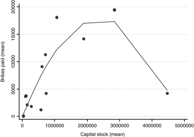
Figure 2 depicts the relationship between firm size and reported bribe payments for a representative cross-section of firms in Uganda (see Svensson Reference Svensson2003 for details).Footnote ³⁰ The data are collapsed at industry level (three-digit ISIC categories) and show that bribes increase in the firm's stock of capital as predicted by Proposition 1, but that the largest firms pay small amounts in bribes. This inverted U-shaped relationship between capital and bribes is as predicted by our model.

FIGURE 2.

Relationship between Bribes Paid and Industry Size

The Macro Level: Corruption in Poor Countries, Lobbying in Rich, and the Poverty Trap

By far the most robust and consistent finding of the empirical cross-country work on corruption is the close relationship between economic development and (perceived) corruption (Treisman Reference Treisman2007). Our model can account for this pattern, as it predicts an evolution where firms bribe at low levels of development but lobby in richer societies. Although cross-country data on lobbying are much more scarce, Campos and Giovannoni (Reference Campos and Giovannoni2007, 15), using the 1999 BEEPS data, conclude that “lobbying is positively associated with the level of economic development.” Consistent with our introductory quote from the International Herald Tribune, their finding suggests that the switch from bribery to lobbying is not specific to high-income countries.

In our model, the evolution from bribery to lobbying is not certain, however. The holdup problem associated with corruption can prevent firms from investing enough to make a switch to lobbying worthwhile. If the regulation is mainly in place to collect bribes, and if the underlying productivity in the economy is not sufficiently high, the result will be a poverty trap. Although this proposition is difficult to test empirically, note that the most corrupt countries according to the World Bank's Control of Corruption index—the most comprehensive cross-country data set on (perceptions of) corruption—have characteristics suggesting that they may indeed by stuck in a poverty trap: they have low income, low growth, and to the extent we can measure it, intrusive business regulations.Footnote ³¹

The Evolution of Regulation

Proposition 7 suggests that the regulatory framework tends to become more “efficient” with development, because sufficiently good rules are never relaxed by lobbying. To exemplify, consider two types of regulations: one put in place out of public interest and another instituted to provide bureaucrats with the power to demand bribes. Propositions 6 and 7 state that firms are more likely to eventually, or at an earlier point in time, lobby for the removal of the “bad” regulations, whereas the “good” regulations are less likely to be relaxed. This could explain why regulations that safeguard public health in Europe and the United States, for instance, although costly for firms to comply with, have not been overturned by corporate lobbying. The prediction is also consistent with the regulation of trade and the regulation of entry of firms. In both cases we observe a significant liberalization over time (as is efficient, we would argue). For example, in the period 1970–1989, 70% of the countries classified by Sach and Warner (Reference Sachs and Warner1995) were closed. In the period 1990–1999, this number has fallen to below 30% (Wacziarg and Welch Reference Wacziarg and Welch2008). Interestingly, the mean annual growth rate from 1970 to the reform date was significantly higher in the reforming countries than in those not reforming during the period, suggesting that, as income grows, the pressure to relax costly regulations increases. The Doing Business dataset covers a much shorter time period but, qualitatively, the results are similar. Of 287 reforms of business regulations in 131 economies introduced between June 2008 through May 2009, only 3 countries introduced rules to make it more difficult to start a firm. Furthermore, cross sectionally, the regulations of entry is closely related to income: rich countries regulate entry less, consistent with our claim that the regulatory framework tends to become more efficient with development (Djankov et al. Reference Djankov, Porta, Lopez-De-Silanes and Shleifer2002).

Penalties for Corruption

The section on policy instruments (Mitigating Corruption: Endogenizing the Policies) provides both normative and positive predictions. Tough penalties on corruption, for example, lead to larger bribes and thus lower investments in a bribery equilibrium. This result is consistent with the findings in Fjeldstad (Reference Fjeldstad2003, Reference Fjeldstad and Rose-Ackerman2006). He studies the reforms of the tax administrations in Tanzania and Uganda. The reforms increased salaries for tax officials and relaxed rules for firing, thus raising the opportunity cost for bureaucrats to accept bribes and making it easier to get fired if caught taking bribes. This did not result in less but, if anything, more corruption. Fjeldstad is also reporting evidence from a PriceWaterhouseCoopers survey of firms in Dar es Salaam that indicates that the price per bribe rose following the reform.

In early phases of development, tough penalties on corruption can prolong the period in which firms choose to bribe by reducing the incentives to invest. Thus, from a normative point of view, our model suggests that the penalty for corruption should be lower in poor countries. Furthermore, it suggests that policies aimed at boosting productivity (r in the model) may be a better approach to reducing corruption because they make a switch from bribery to lobbying more likely and at an earlier point in time through its effect on capital accumulation.