1 Introduction
The injection of a small amount of a low-viscosity fluid inside a pipeline used for the transportation of a high-viscosity fluid induces a remarkable drag reduction (DR). This effect is attributed to the natural tendency of the low-viscosity fluid to migrate towards the high shear wall region, so to create a thin and stable layer which lubricates the wall (Joseph et al.
Reference Joseph, Bai, Chen and Renardy1997). This DR mechanism, originally patented for the industrially relevant case of water-lubricated oil transportation inside pipelines (Isaac & Speed Reference Isaac and Speed1904; Looman Reference Looman1916), was later carefully described and analysed in a series of influential scientific works (see Joseph, Renardy & Renardy Reference Joseph, Renardy and Renardy1984; Oliemans & Ooms Reference Oliemans, Ooms, Hewitt, Delhaye and Zuber1986; Joseph & Renardy Reference Joseph and Renardy1993; Bai, Kelkar & Joseph Reference Bai, Kelkar and Joseph1996; Bannwart Reference Bannwart2001, among others). A comprehensive overview on the topic is provided by Joseph et al. (Reference Joseph, Bai, Chen and Renardy1997) and by Ghosh, Mandal & Das (Reference Ghosh, Mandal and Das2009). According to the global picture emerging from the available literature, the DR mechanism is purely viscosity-driven, with the role of surface tension left unclear. With this work, we want first to demonstrate the crucial role of surface tension in modifying momentum transfer rates and the corresponding overall drag in the considered lubricated channel, and second, to identify the different DR mechanisms, which ultimately depend on the possibility to have a laminar or turbulent lubricating layer near the wall. Finally, we underline the need to extend further the range of parameters to achieve a full understanding of the investigated DR mechanisms. To do this, we start from a simplified and yet relevant simulation setting: We consider a plane channel in which a thin layer of a less-viscous fluid moves on top of a thicker layer of a more-viscous transported fluid. To single out at best the role of surface tension, we also examine the case of a lubricating layer of exactly the same viscosity of the transported fluid. This case will be used as benchmark for the other cases. In this work, we consider a lubricating layer, the thickness of which is
 $7.5\,\%$
of the entire channel height. We use a finely resolved pseudospectral direct numerical simulation (DNS) of turbulence, coupled with a phase field method (PFM) to describe the interactions between the two liquid layers and to track the motion of the liquid–liquid interface. The novel contribution of the present work is the original investigation on the effect of larger viscosity contrast of the lubricating layer: in this way, we can examine two different DR mechanisms, corresponding to flows in which the lubricating layer is laminar for higher viscosity, and turbulent for lower viscosity. In our previous works (Ahmadi et al.
Reference Ahmadi, Roccon, Zonta and Soldati2018a
,Reference Ahmadi, Roccon, Zonta and Soldati
b
), we examined the effect of a fully relaminarized lubricating layer on a marginally turbulent/transitional channel flow (
 $Re_{\unicode[STIX]{x1D70F}}=100$
). To demonstrate that DR can be found also in presence of a lubricating layer in turbulent flow, we run original simulations at
 $Re_{\unicode[STIX]{x1D70F}}=300$
. In order to sustain turbulence in the lubricating layer, we reduce its viscosity down to
 $\unicode[STIX]{x1D702}_{1}=0.25\unicode[STIX]{x1D702}_{2}$
. Our results show that when the viscosity of the two fluids is the same, we can observe a strong DR (
 ${\sim}27\,\%$
), which is due just to the presence of a localized elasticity element – the surface tension of the interface. In this case, we also observe relaminarization of the thin lubricating layer. When we decrease the viscosity of the lubricating layer, we report a DR of
 ${\sim}24\,\%$
, just marginally smaller than the previous case, but we also observe a fully turbulent lubricating layer. Clearly, DR mechanisms are different in the two cases and must correspond to different outcomes in the interplay between viscous forces, inertial forces and surface-generated capillary forces. Using quantitative statistics, and qualitative insights into the relevant phenomena governing the turbulence regeneration cycle, we are able to explain in detail this twofold DR mechanism, which, to the best of our knowledge, has not been investigated before.
2 Methodology
We focus on a flow configuration consisting of two immiscible fluid layers that are driven by an imposed pressure gradient in a horizontal channel. Channel dimensions are
 $L_{x}\times L_{y}\times L_{z}=4\unicode[STIX]{x03C0}h\times 2\unicode[STIX]{x03C0}h\times 2h$
, with
 $h$
the half-channel height and
 $x$
,
 $y$
,
 $z$
the streamwise, spanwise and wall-normal directions, respectively. A thin fluid layer (layer 1),
 $0.15h$
thick, flows over a thicker fluid layer (layer 2),
 $1.85h$
thick. The two layers have different viscosities,
 $\unicode[STIX]{x1D702}_{1}$
and
 $\unicode[STIX]{x1D702}_{2}$
, but the same density,
 $\unicode[STIX]{x1D70C}_{1}=\unicode[STIX]{x1D70C}_{2}=\unicode[STIX]{x1D70C}$
. The deformable interface separating the two fluid layers is characterized by a constant and uniform value of the surface tension
 $\unicode[STIX]{x1D70E}$
. The flow physics, modelled by a PFM, is described by the following set of dimensionless governing balance equations:
 $$\begin{eqnarray}\displaystyle & \displaystyle \unicode[STIX]{x1D735}\boldsymbol{\cdot }\boldsymbol{u}=0, & \displaystyle\end{eqnarray}$$
 $$\begin{eqnarray}\displaystyle & \displaystyle \frac{\unicode[STIX]{x2202}\boldsymbol{u}}{\unicode[STIX]{x2202}t}+\boldsymbol{u}\boldsymbol{\cdot }\unicode[STIX]{x1D735}\boldsymbol{u}=-\unicode[STIX]{x1D735}p+\frac{1}{Re_{\unicode[STIX]{x1D70F}}}\unicode[STIX]{x1D735}\boldsymbol{\cdot }[\unicode[STIX]{x1D702}(\unicode[STIX]{x1D719},\unicode[STIX]{x1D706})(\unicode[STIX]{x1D735}\boldsymbol{u}+\unicode[STIX]{x1D735}\boldsymbol{u}^{\text{T}})]+\frac{3}{\sqrt{8}}\frac{Ch}{We}\unicode[STIX]{x1D735}\boldsymbol{\cdot }\unicode[STIX]{x1D64F}_{c}, & \displaystyle\end{eqnarray}$$
 $$\begin{eqnarray}\displaystyle & \displaystyle \frac{\unicode[STIX]{x2202}\unicode[STIX]{x1D719}}{\unicode[STIX]{x2202}t}+\boldsymbol{u}\boldsymbol{\cdot }\unicode[STIX]{x1D735}\unicode[STIX]{x1D719}=\frac{1}{Pe}\unicode[STIX]{x1D6FB}^{2}(\unicode[STIX]{x1D719}^{3}-\unicode[STIX]{x1D719}-Ch^{2}\unicode[STIX]{x1D6FB}^{2}\unicode[STIX]{x1D719}), & \displaystyle\end{eqnarray}$$
 $\boldsymbol{u}=(u_{x},u_{y},u_{z})$
is the velocity vector,
 $\unicode[STIX]{x1D735}p$
is the pressure gradient (including also the mean pressure gradient that drives the flow, see Soldati & Banerjee Reference Soldati and Banerjee1998),
 $\unicode[STIX]{x1D719}$
is the order parameter which ranges from
 $\unicode[STIX]{x1D719}=-1$
, in one phase, to
 $\unicode[STIX]{x1D719}=1$
, in the other phase, and
 $\unicode[STIX]{x1D706}=\unicode[STIX]{x1D702}_{1}/\unicode[STIX]{x1D702}_{2}$
is the viscosity ratio. Fluid velocity is made dimensionless using the friction velocity
 $$\begin{eqnarray}u_{\star }=\sqrt{\frac{h}{\unicode[STIX]{x1D70C}}\frac{|\text{d}P|}{\text{d}x}}=\sqrt{\frac{|\unicode[STIX]{x1D70F}_{w,1}|+|\unicode[STIX]{x1D70F}_{w,2}|}{2\unicode[STIX]{x1D70C}}}\end{eqnarray}$$
as reference, with
 $\unicode[STIX]{x1D70F}_{w,1}$
and
 $\unicode[STIX]{x1D70F}_{w,2}$
the shear stress at the top and bottom walls, respectively. Note that for the present flow configuration, the thin layer (which we will also refer to as the lubricating layer) is characterized by a viscosity that is always smaller than or equal to that of the thicker layer (which we will also refer to as the main layer), such that
 $\unicode[STIX]{x1D706}\leqslant 1$
. The term
 $\unicode[STIX]{x1D702}(\unicode[STIX]{x1D719},\unicode[STIX]{x1D706})$
in (2.1b
) defines the non-dimensional viscosity distribution inside the domain (Ding, Spelt & Shu Reference Ding, Spelt and Shu2007; Kim Reference Kim2012), whereas the term
 $3Ch/(\sqrt{8}We)\unicode[STIX]{x1D735}\boldsymbol{\cdot }\unicode[STIX]{x1D64F}_{c}$
represents the capillary force per unit mass due to surface tension, with
 $\unicode[STIX]{x1D64F}_{c}=|\unicode[STIX]{x1D735}\unicode[STIX]{x1D719}|^{2}\unicode[STIX]{x1D644}-\unicode[STIX]{x1D735}\unicode[STIX]{x1D719}\otimes \unicode[STIX]{x1D735}\unicode[STIX]{x1D719}$
. Equation (2.1c
), usually called Cahn–Hilliard (CH) equation, describes the transport of the order parameter
 $\unicode[STIX]{x1D719}$
. The term on the right-hand side of (2.1c
) is a diffusive flux that controls the interface behaviour (Badalassi, Ceniceros & Banerjee Reference Badalassi, Ceniceros and Banerjee2003). Dimensionless numbers in (2.1c
)–(2.1b
) are the following: the shear Reynolds number,
 $Re_{\unicode[STIX]{x1D70F}}=\unicode[STIX]{x1D70C}u_{\unicode[STIX]{x1D70F}}h/\unicode[STIX]{x1D702}_{2}$
, which is the ratio between inertial and viscous forces (computed using the viscosity
 $\unicode[STIX]{x1D702}_{2}$
as reference); the Weber number,
 $We=\unicode[STIX]{x1D70C}u_{\unicode[STIX]{x1D70F}}^{2}h/\unicode[STIX]{x1D70E}$
, which is the ratio between inertial and surface tension forces; the Péclet number,
 $Pe=u_{\unicode[STIX]{x1D70F}}h/{\mathcal{M}}\unicode[STIX]{x1D6FD}$
, which is a numerical parameter that controls the interface relaxation time and is defined in terms of
 ${\mathcal{M}}$
, the Onsager coefficient or mobility, and of
 $\unicode[STIX]{x1D6FD}$
, a numerical factor used during the non-dimensionalization of the CH equation; and finally the Cahn number,
 $Ch=\unicode[STIX]{x1D709}/h$
, which represents the dimensionless thickness of the liquid–liquid interface (whose dimensional value is
 $\unicode[STIX]{x1D709}$
). The governing equations are discretized using a pseudospectral method based on transforming the field variables into wavenumber space, through Fourier representations for the periodic (homogeneous) directions
 $x$
and
 $y$
, and a Chebyshev representation for the wall-normal (non-homogeneous) direction
 $z$
. Periodicity along
 $x$
and
 $y$
is assumed for both velocity
 $\boldsymbol{u}$
and order parameter
 $\unicode[STIX]{x1D719}$
, while no-slip (
 $\boldsymbol{u}$
) and no-flux (
 $\unicode[STIX]{x1D719}$
) conditions are imposed at the two walls. Further details on the numerical method can be found in Roccon et al. (Reference Roccon, De Paoli, Zonta and Soldati2017) and Soligo, Roccon & Soldati (Reference Soligo, Roccon and Soldati2019).
2.1 Simulation set-up
We considered four different cases. The benchmark single-phase flow case and three different cases of viscosity-stratified two-phase flow, each characterized by a different value of the viscosity ratio
 $\unicode[STIX]{x1D706}$
. Specifically, we considered
 $\unicode[STIX]{x1D706}=1$
,
 $\unicode[STIX]{x1D706}=0.5$
and
 $\unicode[STIX]{x1D706}=0.25$
. All simulations are run at the given reference value of the shear Reynolds number
 $Re_{\unicode[STIX]{x1D70F}}=300$
and Weber number
 $We=0.5$
. These values of the flow parameters correspond to a physical situation (planned in our experimental lab) in which water is used to lubricate a main layer of light oil (Exxon Mobil Solvesso 200 ND) characterized by density
 $\unicode[STIX]{x1D70C}_{2}=980~\text{kg}~\text{m}^{-3}$
, viscosity
 $\unicode[STIX]{x1D702}_{2}=3.85\times 10^{-3}~\text{Pa}~\text{s}$
and surface tension
 $\unicode[STIX]{x1D70E}\simeq 44\times 10^{-3}~\text{N}~\text{m}^{-1}$
. Assuming a channel with
 $h=6\times 10^{-2}~\text{m}$
, the bulk velocity and the shear velocity become
 $u_{b}=0.32~\text{m}~\text{s}^{-1}$
and
 $u_{\unicode[STIX]{x1D70F}}=0.0194~\text{m}~\text{s}^{-1}$
, respectively. The grid resolution has been chosen so to fulfil requirements imposed by DNS. When the fluid viscosity changes, spatial flow scales become smaller and the computational grid must be refined accordingly (Zonta, Marchioli & Soldati Reference Zonta, Marchioli and Soldati2012). For the single-phase case and for the case
 $\unicode[STIX]{x1D706}=1$
, we used
 $N_{x}\times N_{y}\times N_{z}=512\times 256\times 257$
; for the case
 $\unicode[STIX]{x1D706}=0.50$
we used
 $512\times 512\times 513$
; for the case
 $\unicode[STIX]{x1D706}=0.25$
we used
 $1024\times 1024\times 513$
. The Cahn number is set to
 $Ch=0.02$
, while the Péclet number is obtained according to the scaling
 $Pe=3/Ch$
(Jacqmin Reference Jacqmin1999). The initial condition for the two-phase flow simulations is taken from a preliminary DNS of single-phase fully developed turbulent channel flow at
 $Re_{\unicode[STIX]{x1D70F}}=300$
, complemented by a proper definition of the initial distribution of the order parameter
 $\unicode[STIX]{x1D719}$
so that the liquid–liquid interface is initially flat and located at distance
 $0.15h$
from one wall.
3 Results
We characterize the flow both from qualitative and quantitative viewpoints, so to gain physically grounded understanding of the competition between viscous forces, inertial forces and surface-generated capillary forces in damping and sustaining the turbulence structures in the lubricating layer.
3.1 Flow rates and mean velocity profiles
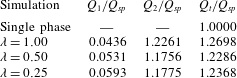
We computed the volumetric flow rate of each liquid layer,
 $Q_{1}$
and
 $Q_{2}$
, and we normalized it by the value of the volume flow rate of the single-phase flow
 $Q_{sp}$
. We recall that
 $Q_{1}$
is the flow rate of the lubricating layer, while
 $Q_{2}$
is the flow rate of the main transported fluid. Results are presented in table 1. Compared to the single-phase case, we underline the increase of both
 $Q_{1}$
and
 $Q_{2}$
(and of the total flow rate
 $Q_{t}=Q_{1}+Q_{2}$
as well), which is the footprint of the DR induced by the injection of the surface-tension-active lubricating layer. The increase of the volume flow rate of the main fluid,
 $Q_{2}$
, is not monotonic with decreasing
 $\unicode[STIX]{x1D706}$
: The fractional increase of
 $Q_{2}$
(
 $\unicode[STIX]{x0394}Q_{2}/Q_{SP}=(Q_{2}-Q_{SP})/Q_{SP}$
) is maximum for
 $\unicode[STIX]{x1D706}=1$
and marginally lower for
 $\unicode[STIX]{x1D706}=0.5$
and
 $\unicode[STIX]{x1D706}=0.25$
. The flow rate of the lubricating layer,
 $Q_{1}$
, increases steadily for decreasing
 $\unicode[STIX]{x1D706}$
.
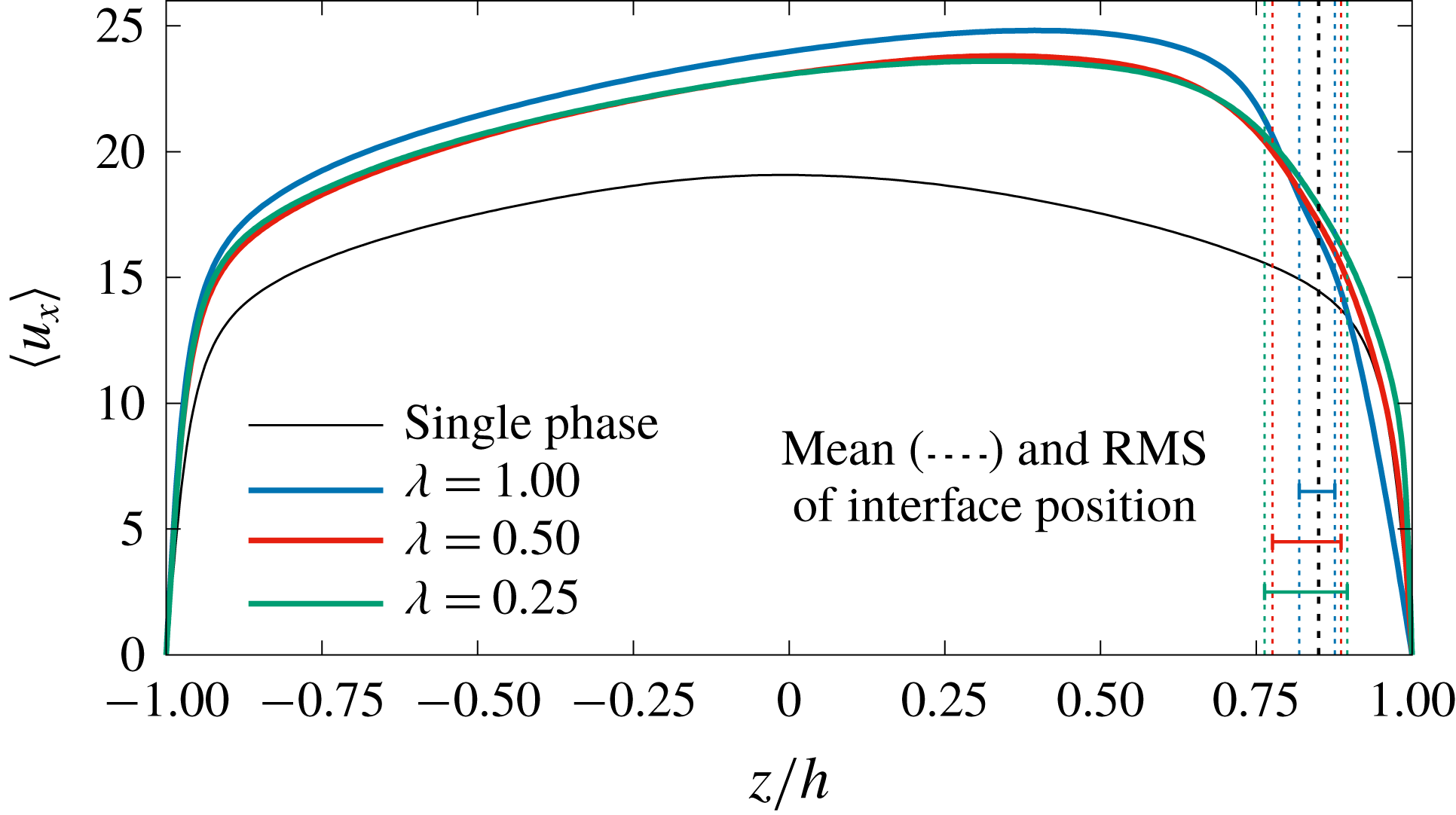
Mean fluid streamwise velocity,
 $\langle u_{x}\rangle$
, in the wall-normal direction for the different cases considered in the present study. Comparison between the benchmark single-phase case (SP, solid black line), and the lubricated channel with
 $\unicode[STIX]{x1D706}=1.00$
(solid blue line),
 $\unicode[STIX]{x1D706}=0.50$
(solid red line) and
 $\unicode[STIX]{x1D706}=0.25$
(solid green line). The mean interface position (
 $z/h=0.85$
) and the corresponding RMS values of the interface displacement are indicated by dashed lines.

Volume flow rate of the lubricating layer (layer 1,
 $Q_{1}$
) and of the main layer (layer 2,
 $Q_{2}$
) for the different values of the viscosity ratio
 $\unicode[STIX]{x1D706}$
considered in the present study. The total volume flow rate (
 $Q_{t}=Q_{1}+Q_{2}$
) is also evaluated. Results for the benchmark single-phase case are included for comparison. All values are normalized by the volume flow rate of the single-phase case,
 $Q_{SP}$
.

In figure 1 we show, for the different examined cases, the profile of the mean streamwise velocity
 $\langle u_{x}\rangle$
expressed in wall units and averaged over time and space (in the homogeneous directions,
 $x$
and
 $y$
). It is beyond the scope of the present paper to fully characterize the interactions between interface deformation and turbulence fluctuations. However, to sketch the dynamics of the interface, we report in figure 1 the average position of the interface, and positive and negative RMS values of interface displacement, which are the average height and depth of crests and troughs of interfacial waves. It is important to observe that, due to wall confinement, fluctuations towards the centre of the channel (wave troughs) are larger than fluctuations towards the wall (wave crests). It is also interesting to observe that reducing
 $\unicode[STIX]{x1D706}$
corresponds to an increase of the average interface deformation. For the values of
 $\unicode[STIX]{x1D706}$
investigated, the presence of the thin lubricating layer produces a skewed asymmetric velocity profile. Focusing first on the main layer (
 $z/h<0.85$
), we observe that the maximum velocity increment corresponds to
 $\unicode[STIX]{x1D706}=1$
. Decreasing
 $\unicode[STIX]{x1D706}$
to
 $0.5$
corresponds to a more limited increase of the average velocity compared to the single-phase case. Decreasing further
 $\unicode[STIX]{x1D706}$
to
 $0.25$
induces only negligible modifications to the velocity profile, which indeed remains very close to that of the case
 $\unicode[STIX]{x1D706}=0.5$
. Focusing now on the lubricating layer (
 $z/h>0.85$
), we observe a strong, monotonic, increase of the velocity gradient for decreasing
 $\unicode[STIX]{x1D706}$
. The difference of the velocity gradients at the wall indicates a flow behaviour in the lubricating layer that changes with
 $\unicode[STIX]{x1D706}$
and that seems to suggest a different phenomenology for the DR mechanisms. Considering the similarity of the velocity profiles for
 $\unicode[STIX]{x1D706}=0.5$
and
 $\unicode[STIX]{x1D706}=0.25$
, and in order to simplify the discussion, in the following we will focus only on the cases
 $\unicode[STIX]{x1D706}=1$
and
 $\unicode[STIX]{x1D706}=0.25$
.
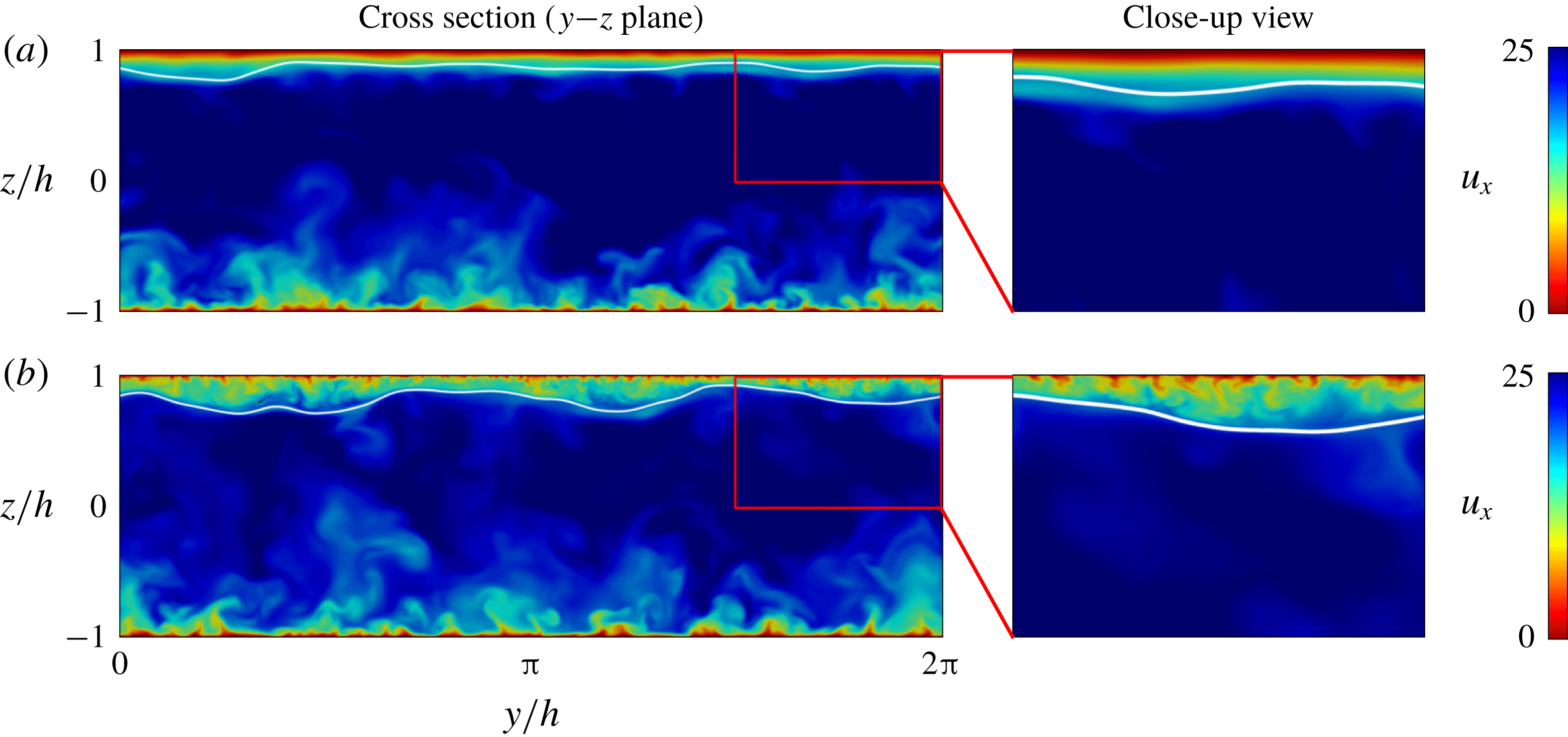
In figure 2 we show the instantaneous streamwise velocity field in the channel cross-section
 $(y-z)$
for
 $\unicode[STIX]{x1D706}=1$
(figure 2
a) and
 $\unicode[STIX]{x1D706}=0.25$
(figure 2
b). The white line indicates the instantaneous position of the interface. In figure 2(a), we notice the presence of turbulence structures (Schoppa & Hussain Reference Schoppa and Hussain2002; Jiménez Reference Jiménez2013) at the bottom wall (
 $z/h=-1$
), but we see no evidence of turbulence at the top wall (
 $z/h=1$
); this can be appreciated better in the corresponding close-up view. Turning to figure 2(b), we observe turbulence structures at both walls. In particular, from the close-up view, we appreciate that typical turbulence structures still populate the flow region near the top wall. It is then clear that the DR observed for the case
 $\unicode[STIX]{x1D706}=1$
can be attributed to the relaminarization of the lubricating layer, in which turbulence is totally damped. The clear existence of turbulence in the case
 $\unicode[STIX]{x1D706}=0.25$
(figure 2
b) demonstrates that the velocity gradients of figure 1 are steeper due to the persistence of the turbulence near the wall, but calls for a different DR mechanism. On a qualitative basis, we also observe that turbulence structures in the low-viscosity lubricating layer (case
 $\unicode[STIX]{x1D706}=0.25$
) appear smaller than those at the bottom wall. A detailed characterization of the turbulence scales at the two walls will be the object of a future analysis.
Instantaneous streamwise velocity
 $u_{x}$
in a cross-section (
 $y$
–
 $z$
) of the channel. Panel (a) refers to the case
 $\unicode[STIX]{x1D706}=1$
whereas panel (b) refers to the case
 $\unicode[STIX]{x1D706}=0.25$
. The position of the interface is explicitly indicated by a thin white line. For both values of
 $\unicode[STIX]{x1D706}$
, a close-up view of a rectangular region near the top wall is also offered to appreciate the different flow structure (complete turbulence suppression for
 $\unicode[STIX]{x1D706}=1$
and sustained turbulence for
 $\unicode[STIX]{x1D706}=0.25$
).

3.2 Stress behaviour
In this subsection, we aim at studying in detail the role of the interface and its implications on the overall stress distribution in the wall-normal direction. The average of the total stress as a function of the wall-normal coordinate reads
 $$\begin{eqnarray}\unicode[STIX]{x1D70F}_{tot}=\underbrace{\frac{\langle \unicode[STIX]{x1D702}(z)\rangle }{Re_{\unicode[STIX]{x1D70F}}}\frac{\unicode[STIX]{x2202}\langle u_{x}\rangle }{\unicode[STIX]{x2202}z}}_{\unicode[STIX]{x1D70F}_{v}}-\underbrace{\langle u_{x}^{\prime }u_{z}^{\prime }\rangle }_{\unicode[STIX]{x1D70F}_{t}}+\underbrace{\frac{3}{\sqrt{8}}\frac{Ch}{We}\left\langle \frac{\unicode[STIX]{x2202}\unicode[STIX]{x1D719}}{\unicode[STIX]{x2202}x}\frac{\unicode[STIX]{x2202}\unicode[STIX]{x1D719}}{\unicode[STIX]{x2202}z}\right\rangle }_{\unicode[STIX]{x1D70F}_{c}}.\end{eqnarray}$$
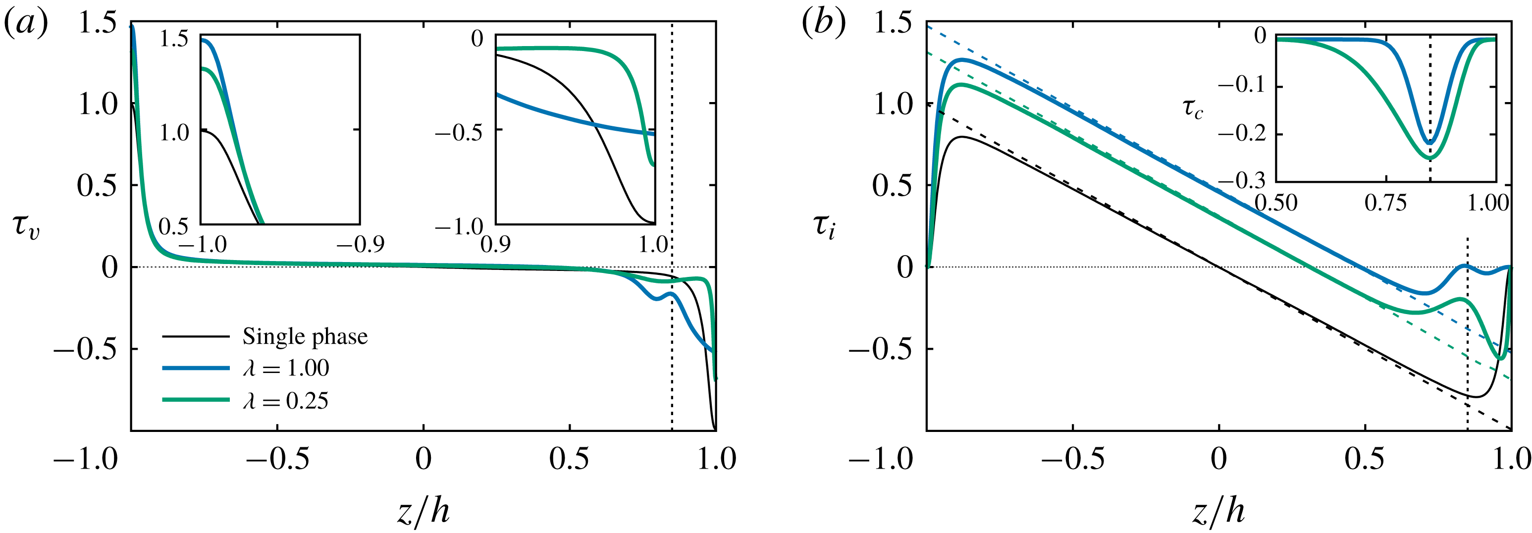
(a) Wall-normal behaviour of the viscous shear stress,
 $\unicode[STIX]{x1D70F}_{v}$
, for the two cases
 $\unicode[STIX]{x1D706}=1$
(blue line) and
 $\unicode[STIX]{x1D706}=0.25$
(green line). The viscous shear stress for the reference single-phase case (black thin line) is also shown for comparison. A close-up view of
 $\unicode[STIX]{x1D70F}_{v}$
in the near-wall regions is also given in the insets. The average interface position (
 $z/h=0.85$
) is explicitly indicated by a vertical dashed line. (b) Wall-normal behaviour of the turbulent shear stress,
 $\unicode[STIX]{x1D70F}_{t}$
, and of the total shear stress
 $\unicode[STIX]{x1D70F}_{tot}$
(linear profile drawn using dashed lines) for the single-phase case and for
 $\unicode[STIX]{x1D706}=1$
and
 $\unicode[STIX]{x1D706}=0.25$
. The behaviour of the capillary stress
 $\unicode[STIX]{x1D70F}_{c}$
in the region near the interface is given in the inset. Lines as in (a).

In the case under examination, the total stress
 $\unicode[STIX]{x1D70F}_{tot}$
comprises the viscous shear stress,
 $\unicode[STIX]{x1D70F}_{v}$
, the turbulent shear stress,
 $\unicode[STIX]{x1D70F}_{t}$
, and the capillary stress,
 $\unicode[STIX]{x1D70F}_{c}$
. For an easier examination, we plot these three contributions, as well as their sum, in figure 3. In figure 3(a), we plot the profiles of the viscous shear stress, highlighting in the insets their zoomed-out behaviour near the walls. We underline here that the pressure gradient driving the flow is equivalent to the sum of the values of the viscous shear stress at the two walls (this sum is equal to 2 in our dimensionless notation). The pressure gradient driving the flow, and consequently this sum, are kept constant for all our simulations. The viscous shear stress near the bottom wall (
 $z/h<-0.9$
in figure 3
a, and inset on the left) has the shape typical of near-wall turbulence for all examined cases, although the value of the wall shear stress is clearly different, being
 $\unicode[STIX]{x1D70F}_{v}=1$
(black thin line) for the single-phase case,
 $\unicode[STIX]{x1D70F}_{v}=1.47$
for
 $\unicode[STIX]{x1D706}=1$
(blue line) and
 $\unicode[STIX]{x1D70F}_{v}=1.34$
for
 $\unicode[STIX]{x1D706}=0.25$
(green line). The behaviour of the viscous shear stress near the top wall (
 $z/h=\,>0.9$
in figure 3
a, and inset on the right), however, shows some important differences. While for
 $\unicode[STIX]{x1D706}=0.25$
the behaviour is similar, but shifted downwards (in magnitude), compared to the single-phase case, the behaviour for
 $\unicode[STIX]{x1D706}=1$
displays a quasi-linear profile typical of a relaminarized layer. It is also important to observe that the viscous shear stress crossing the nominal position of the interface has a non-trivial behaviour characterized by a local minimum (in magnitude) which, as from (3.1), must be balanced by a corresponding behaviour of the other two terms. In figure 3(b), we show the behaviour of the turbulent stress, and, in the inset, the behaviour of the capillary stress,
 $\unicode[STIX]{x1D70F}_{c}$
: the region plotted in this inset is the only region where the capillary stress is different from zero. The turbulent shear stress shows a clear asymmetry, which corresponds closely to that of the mean velocity observed in figure 1, but also to that visible in the viscous shear stress figure 3(a). In the main layer (
 $z/h<0.85$
), the turbulent stresses for examined cases have the typical shape of wall-bounded turbulence, with only the profiles amplitude differing among each other. In the interface region, we observe local minima for both cases. For
 $\unicode[STIX]{x1D706}=1$
(blue line), the turbulent stress is nearly zero, and the observed local minimum in the viscous shear stress (figure 3
a) is almost fully balanced by the capillary stress, shown by the blue line in the inset. For
 $\unicode[STIX]{x1D706}=0.25$
(green line), the turbulent stress reaches a local minimum, larger than zero (in absolute value), which, due to the corresponding negligible value of the viscous shear stress in this region (figure 3
a), is almost fully balanced by the capillary stress (green line in the inset of figure 3). In both cases, the capillary stress is the crucial element in the DR process. In the
 $\unicode[STIX]{x1D706}=1$
case, the capillary stress decouples the dynamics of the main fluid layer from that of the lubricating layer, which eventually relaminarizes. In the
 $\unicode[STIX]{x1D706}=0.25$
case, the capillary stress also decouples the dynamics of the main fluid layer from that of the lubricating layer, but a residual turbulent stress flux is maintained through the interface, which now separates two layers both characterized by turbulent flow. Reportedly (Jiménez & Moin Reference Jiménez and Moin1991), turbulence in channel flow can be sustained if the shear Reynolds number is above
 ${\sim}90$
. We have seen from figure 3 that the interface, via the action of the capillary stress, is a strong separation element between the main layer and the lubricating layer. Although the interface is compliant, it is capable of exerting some stress, and therefore we can idealize the flow in the lubricating layer as a separate channel flow characterized by a nominal height of
 $h_{l}^{+}$
. We remark here that wall scales are changed by the change of viscosity, and their new values can be determined using the steady-state value of the wall shear stress. So, even if the thickness of the lubricating layer is constant in outer units, it changes if expressed in wall units according to the local value of the shear stress which establishes at the top wall. In this situation, the dimensionless thickness of the lubricating layer can be obtained via a semi-local scaling (using reference quantities computed at the top wall only, see Pecnik & Patel Reference Pecnik and Patel2017) as
 $$\begin{eqnarray}h_{l}^{+}=0.15\frac{Re_{\unicode[STIX]{x1D70F}}}{\unicode[STIX]{x1D706}}\sqrt{\frac{2|\unicode[STIX]{x1D70F}_{w,1}|}{|\unicode[STIX]{x1D70F}_{w,1}|+|\unicode[STIX]{x1D70F}_{w,2}|}}.\end{eqnarray}$$
For
 $\unicode[STIX]{x1D706}=1$
, we obtain
 $h_{l}^{+}=33$
: this value indicates that the lubricating layer is not large enough to sustain turbulence (Jiménez & Moin Reference Jiménez and Moin1991). For
 $\unicode[STIX]{x1D706}=0.25$
, we obtain
 $h_{l}^{+}=145$
, which is definitely enough to sustain turbulence. The intermediate simulation at
 $\unicode[STIX]{x1D706}=0.5$
(not shown here) is characterized by a threshold value for the channel height of approximately 73 wall units. Since the steady-state values of the shear stresses are not known a priori, to design new simulations one can use the reference parameters of the single-phase simulation and rescale the thickness of the lubricating layer with the new viscosity values: in this way we obtain
 $h_{l}^{+}=45$
for
 $\unicode[STIX]{x1D706}=1$
,
 $h_{l}^{+}=45/\unicode[STIX]{x1D706}=90$
for
 $\unicode[STIX]{x1D706}=0.5$
and
 $h_{l}^{+}=45/\unicode[STIX]{x1D706}=180$
for
 $\unicode[STIX]{x1D706}=0.25$
.
3.3 Probability density function (PDF) of the wall shear stress
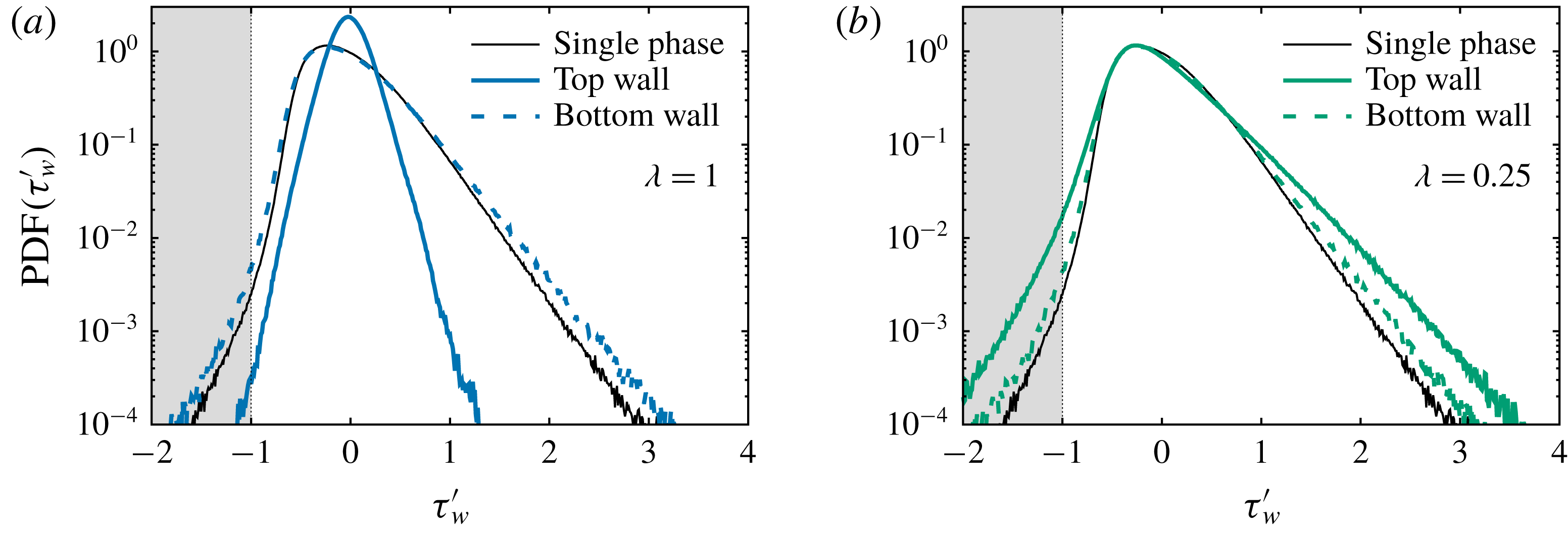
Further evidence of the DR mechanisms can be obtained examining the distribution of the wall shear stress
 $\unicode[STIX]{x1D70F}_{w}$
at the two walls. We compute the probability density function (PDF) of the wall shear stress fluctuations
 $\unicode[STIX]{x1D70F}_{w}^{\prime }$
, and we normalize it by the mean value
 $\langle \unicode[STIX]{x1D70F}_{w}\rangle$
of the shear stress at the corresponding wall, i.e.
 $\unicode[STIX]{x1D70F}_{w}^{\prime }=(\unicode[STIX]{x1D70F}_{w}-\langle \unicode[STIX]{x1D70F}_{w}\rangle )/\langle \unicode[STIX]{x1D70F}_{w}\rangle$
. Results are shown in figure 4(a) for the case
 $\unicode[STIX]{x1D706}=1$
and in figure 4(b) for the case
 $\unicode[STIX]{x1D706}=0.25$
. The thin solid line refers to the single-phase case, whereas the thick dashed line and the thick solid line refer to the bottom and to the top wall, respectively.
Probability density function (PDF) of the normalized wall shear stress fluctuation
 $\unicode[STIX]{x1D70F}_{w}^{\prime }=(\unicode[STIX]{x1D70F}_{w}-\langle \unicode[STIX]{x1D70F}_{w}\rangle )/\langle \unicode[STIX]{x1D70F}_{w}\rangle$
for
 $\unicode[STIX]{x1D706}=1$
(a) and
 $\unicode[STIX]{x1D706}=0.25$
(b). In each panel, the thick solid line refers to the top wall, whereas the thick dashed line refers to the bottom wall. The behaviour for the single-phase case is shown with a thin black line.

We focus first on the single-phase case. Consistently with previous literature studies (Hu, Morfey & Sandham Reference Hu, Morfey and Sandham2006; Lenaers et al.
Reference Lenaers, Li, Brethouwer, Schlatter and Örlü2012; Brücker Reference Brücker2015), we notice that the PDF
 $(\unicode[STIX]{x1D70F}_{w}^{\prime })$
has an asymmetric and positively skewed shape, which indicates that positive fluctuations are larger in magnitude and occur more frequently than negative fluctuations (the maximum value is
 $\unicode[STIX]{x1D70F}_{w}^{\prime }\simeq 3$
, while the minimum is
 $\unicode[STIX]{x1D70F}_{w}^{\prime }\simeq -1.5$
). Note however that there is a non-negligible probability of observing events characterized by
 $\unicode[STIX]{x1D70F}_{w}^{\prime }<-1$
(shaded region in the picture): these events mark the appearance of localized counter-flow regions in which the instantaneous shear stress changes sign compared to its mean value, and in which the local flow velocity is reversed compared to the mean velocity (localized flow reversal).
We now focus on the case
 $\unicode[STIX]{x1D706}=1$
(figure 4
a). At the bottom wall (dashed blue line), the shape of PDF
 $(\unicode[STIX]{x1D70F}_{w}^{\prime })$
is similar to that of the single-phase case described above, but it becomes slightly wider, indicating that positive (
 $\unicode[STIX]{x1D70F}_{w}^{\prime }>0.5$
) and negative (
 $\unicode[STIX]{x1D70F}_{w}^{\prime }<0.5$
) fluctuations occur more frequently. This effect is known (Lenaers et al.
Reference Lenaers, Li, Brethouwer, Schlatter and Örlü2012) and can be attributed to the local increase of the Reynolds number, which, with arguments similar to those used to derive (3.2), lead to an estimate of
 $Re_{\unicode[STIX]{x1D70F}}\simeq 350$
. At the top wall (blue solid line) the situation changes completely. The PDF
 $(\unicode[STIX]{x1D70F}_{w}^{\prime })$
becomes taller and almost symmetric, narrowing around the most probable value
 $\unicode[STIX]{x1D70F}_{w}^{\prime }=0$
. This indicates that shear stress fluctuations are strongly reduced in magnitude and in frequency. The narrowing of the curve around
 $\unicode[STIX]{x1D70F}_{w}^{\prime }=0$
(collapse of the curve onto
 $\unicode[STIX]{x1D70F}_{w}^{\prime }=0$
) indicates that the local shear stress is approximately equal to the mean shear stress, a further confirmation and a clear signature of the local flow laminarization process in the lubricating layer. Finally, we focus on the case
 $\unicode[STIX]{x1D706}=0.25$
(figure 4
b). The shape of the PDF
 $(\unicode[STIX]{x1D70F}_{w}^{\prime })$
for both the top (green solid line) and bottom wall (green dashed line) recovers the non-symmetric and positively skewed profile valid for the single-phase case (black thin line), which is a further indication that turbulence is active when the viscosity of the lubricating layer is sufficiently small (
 $\unicode[STIX]{x1D706}=0.25$
). We notice that large positive (
 $\unicode[STIX]{x1D70F}_{w}^{\prime }>1$
) and negative (
 $\unicode[STIX]{x1D70F}_{w}^{\prime }<1$
) events occur more frequently in the two-phase case compared to the single-phase case, at both the bottom and the top wall. While the behaviour at the bottom wall is due to the increased local shear Reynolds number (pretty much like in the case
 $\unicode[STIX]{x1D706}=1$
discussed above, figure 4
a), the behaviour at the top wall has a different origin, being ultimately driven by the flow modulation induced by the liquid–liquid interface (Ahmadi et al.
Reference Ahmadi, Roccon, Zonta and Soldati2018a
). The deformed interface is characterized by crests, which push fluid towards the wall (upwashes), and troughs, which draw fluid away from the wall (downwashes). These upward and downward fluid motions induce wall shear stress fluctuations, whose strength and frequency of occurrence is clearly increased consistently, as apparent from the shape of the PDF.
4 Conclusions
In this work, we have confirmed that a lubricating compliant layer can strongly reduce drag in a turbulent channel flow. We have also demonstrated that DR can be driven by surface tension effects alone, or also by a combination of surface tension and viscosity effects if the viscosity of the lubricating layer is smaller than that of the main flow. We studied this problem starting from viscosity-matched fluids and decreasing the viscosity of the lubricating layer. When the two fluids have the same viscosity, the thin lubricating layer relaminarizes due to the lack of the minimal conditions to sustain the near-wall turbulence cycle, and a strong DR is observed. When the viscosity of the lubricating layer is reduced, turbulence in the layer can be sustained, but the overall system drag can still be substantially reduced.
In particular, we have characterized the phenomenology of DR in the present flow configuration by performing DNS at the given shear Reynolds number
 $Re_{\unicode[STIX]{x1D70F}}=300$
, and at three different values of the viscosity ratio
 $\unicode[STIX]{x1D706}=\unicode[STIX]{x1D702}_{1}/\unicode[STIX]{x1D702}_{2}$
between the two fluids (with
 $\unicode[STIX]{x1D702}_{1}$
the viscosity of the fluid in the lubricating layer). We started by focusing on the case
 $\unicode[STIX]{x1D706}=1$
, which we used as reference case to isolate the effect of surface tension on the DR mechanisms, then we lowered the viscosity ratio to
 $\unicode[STIX]{x1D706}=0.5$
and
 $\unicode[STIX]{x1D706}=0.25$
, to analyse the complex interplay between viscous forces, inertial forces and surface-generated capillary forces on the overall DR.
Reduction of drag is as high as
 $\text{DR}\sim 27\,\%$
for
 $\unicode[STIX]{x1D706}=1$
, and, counter to intuition, slightly decreases for decreasing
 $\unicode[STIX]{x1D706}$
(
 $\text{DR}\sim 24\,\%$
for
 $\unicode[STIX]{x1D706}=0.25$
). Based on the current results, we were able to identify two different routes to DR in the present system. When
 $\unicode[STIX]{x1D706}=1$
, DR is due to the surface tension of the interface, which is the elasticity element that decouples wall-normal momentum transfer mechanisms between the main and lubricating layers, leading to a complete relaminarization of the lubricating layer (surface-tension-driven DR), leading to a complete relaminarization of the lubricating layer (surface-tension-driven DR). However, when the viscosity contrast is changed to
 $\unicode[STIX]{x1D706}=0.25$
, and turbulence can still be sustained in the lubricating layer, we can observe a new DR mechanism. In this case, DR is attributed to the effect of lower viscosity of the lubricating layer, which decreases the corresponding value of the wall shear stress (viscosity-driven DR).
In the present study, to minimize the influence of the flow parameters on the results, but at the same time to represent an experimentally and physically realizable situation, we have fixed (among the different simulations) the reference thickness of the lubricating layer (
 $h_{l}=0.15h$
) and the surface tension (
 $\unicode[STIX]{x1D70E}=44\times 10^{-3}~\text{N}~\text{m}^{-1}$
) of the liquid–liquid interface. Further investigations are therefore required to study the role of
 $h_{l}$
and
 $\unicode[STIX]{x1D70E}$
on the proposed turbulence suppression and regeneration mechanisms that determine the overall DR in the present system.
Acknowledgements
Vienna Scientific Cluster (Vienna, Austria) and CINECA Supercomputing Center (Bologna, Italy) are gratefully acknowledged for generous allowance of computer resources under grants 71026 and HP10BCFP82.