1 Introduction
Weak turbulence theory (WTT), developed in the 1960s, provides a mathematical description of the energy transfer in weakly nonlinear and dispersive waves (Zakharov, L’vov & Falkovich Reference Zakharov, L’vov and Falkovich1992; Newell & Rumpf Reference Newell and Rumpf2011). In the framework of WTT, a systematic approach, based on the truncated Hamiltonian, reduces the primitive wave equation to the kinetic equation (KE), which governs the wave spectral evolution due to nonlinear energy transfer. The stationary solution of the KE yields a Kolmogorov–Zakharov spectrum of power-law form in the inertial range. This methodology has been applied in many physical systems, including plasma physics (e.g. Galtier et al. Reference Galtier, Nazarenko, Newell and Pouquet2002), optics (e.g. Dyachenko et al. Reference Dyachenko, Newell, Pushkarev and Zakharov1992), internal waves (e.g. Lvov, Polzin & Tabak Reference Lvov, Polzin and Tabak2004), surface gravity and capillary waves (e.g. Zakharov & Filonenko Reference Zakharov and Filonenko1966, Reference Zakharov and Filonenko1967).
For capillary waves, the KE is first derived in Zakharov & Filonenko (Reference Zakharov and Filonenko1967), and takes the form
 $\unicode[STIX]{x2202}n_{\boldsymbol{k}}/\unicode[STIX]{x2202}t=S(\boldsymbol{k},n_{\boldsymbol{k}})$
, where
 $n_{\boldsymbol{k}}$
is the spectral density of wave action at vector wavenumber
 $\boldsymbol{k}$
and
 $S(\boldsymbol{k},n_{\boldsymbol{k}})\sim \iint _{-\infty }^{\infty }\unicode[STIX]{x1D6FF}(\boldsymbol{k}-\boldsymbol{k}_{1}-\boldsymbol{k}_{2})\unicode[STIX]{x1D6FF}(\unicode[STIX]{x1D714}_{\boldsymbol{k}}-\unicode[STIX]{x1D714}_{\boldsymbol{k}_{1}}-\unicode[STIX]{x1D714}_{\boldsymbol{k}_{2}})\,\text{d}\boldsymbol{k}_{1}\,\text{d}\boldsymbol{k}_{2}$
is the collision integral, representing the nonlinear spectral evolution due to triad resonant interactions, with
 $\unicode[STIX]{x1D714}_{\boldsymbol{k}}\sim |\boldsymbol{k}|^{3/2}$
being the angular frequency.
In an isotropic wavefield, the analytical stationary solution (with large-scale forcing and small-scale dissipation) of the KE yields a power-law spectrum in the inertial range (Zakharov & Filonenko Reference Zakharov and Filonenko1967; Pushkarev & Zakharov Reference Pushkarev and Zakharov2000; Pan & Yue Reference Pan and Yue2014),
 $$\begin{eqnarray}n(k)=2\unicode[STIX]{x03C0}CP^{1/2}k^{\unicode[STIX]{x1D6FC}},\end{eqnarray}$$
where
 $P$
is the energy flux from large to small scales,
 $\unicode[STIX]{x1D6FC}$
is the spectral slope, with the theoretical value of
 $\unicode[STIX]{x1D6FC}=\unicode[STIX]{x1D6FC}_{0}=-17/4$
, and
 $C$
is the Kolmogorov constant, first analytically evaluated in Pushkarev & Zakharov (Reference Pushkarev and Zakharov2000) with a reported value of 9.85. In obtaining (1.1), a key assumption is made of an infinite domain with continuous wavenumber, under which the interaction of a triad satisfies the exact resonance condition
 $$\begin{eqnarray}\displaystyle & \boldsymbol{k}-\boldsymbol{k}_{1}-\boldsymbol{k}_{2}=0, & \displaystyle\end{eqnarray}$$
 $$\begin{eqnarray}\displaystyle & \unicode[STIX]{x1D714}_{\boldsymbol{k}}-\unicode[STIX]{x1D714}_{\boldsymbol{k}_{1}}-\unicode[STIX]{x1D714}_{\boldsymbol{k}_{2}}=0, & \displaystyle\end{eqnarray}$$
 $S(\boldsymbol{k},n_{\boldsymbol{k}})$
takes a non-zero value.
In reality, the assumption of an infinite domain with continuous wavenumber is never realized, and experimental and numerical validations of (1.1) are attempted only in finite domains under the context of discrete turbulence. These include the extensive numerical (e.g. Pushkarev & Zakharov Reference Pushkarev and Zakharov1996, Reference Pushkarev and Zakharov2000; Deike et al.
Reference Deike, Daniel, Berhanu and Falcon2014b
; Pan & Yue Reference Pan and Yue2014) and experimental (e.g. Falcon, Laroche & Fauve Reference Falcon, Laroche and Fauve2007; Xia, Shats & Punzmann Reference Xia, Shats and Punzmann2010; Deike, Berhanu & Falcon Reference Deike, Berhanu and Falcon2014a
) confirmations of
 $\unicode[STIX]{x1D6FC}=\unicode[STIX]{x1D6FC}_{0}=-17/4$
, which can be considered to be settled. Studies to evaluate the value of
 $C$
in (1.1) are less definitive, and it turns out that the value originally reported in Pushkarev & Zakharov (Reference Pushkarev and Zakharov2000) is off by a factor of
 $\sqrt{2}$
, due to an error in evaluating a key integral. In this work, we rederive the analytical solution in § 2, which yields the corrected value of
 $C=C_{0}=6.97$
. This lays down a new premise not only for later study in current work, but also for all previous attempted validations, among which the most recent one (Pan & Yue Reference Pan and Yue2014) should be considered as the recovery of
 $C_{0}$
in the same order of magnitude.
The consideration of nonlinear resonance broadening (NRB) is essential in understanding discrete turbulence since it is mathematically known (Kartashova Reference Kartashova1990) that the exact triad resonance condition (1.2) cannot be satisfied in a finite domain resonator (as (1.2b
) for integer wavenumbers turns into a special case of Fermat’s last theorem). The relationship of NRB (and nonlinearity level) to the dynamics can be argued from a sandpile model (Nazarenko Reference Nazarenko2006; Lvov & Nazarenko Reference Lvov and Nazarenko2010; Nazarenko Reference Nazarenko2011). With increasing magnitude of NRB, the spectral slope varies from that corresponding to frozen, mesoscopic to continuous (kinetic) turbulence. These predictions are consistent with simulations of the primitive Euler equations (Pushkarev & Zakharov Reference Pushkarev and Zakharov2000; Pan & Yue Reference Pan and Yue2014, Reference Pan and Yue2015) and experiments (e.g. Denissenko, Lukaschuk & Nazarenko Reference Denissenko, Lukaschuk and Nazarenko2007; Deike, Bacri & Falcon Reference Deike, Bacri and Falcon2013). In addition to the spectral slope
 $\unicode[STIX]{x1D6FC}<\unicode[STIX]{x1D6FC}_{0}$
, the simulation demonstrates the reduced capacity of energy cascade at insufficient level of nonlinearity, producing spectra with
 $C>C_{0}$
. The problem is also tackled by geometrically considering the formation of quasi-resonant triads with NRB under wavenumber discreteness (e.g. Pushkarev & Zakharov Reference Pushkarev and Zakharov2000; Connaughton, Nazarenko & Pushkarev Reference Connaughton, Nazarenko and Pushkarev2001), and a conclusion is reached that an energy cascade over range of wavenumber is only possible under sufficient NRB. However, a quantitative measure of NRB is still lacking in the context of a realistic wavefield, and its relation with the nonlinearity level and spectral properties is yet to be established. In § 3, we provide such an analysis using data from direct simulation of Euler equations to elucidate the mechanism of NRB in discrete turbulence.
Although the KE is not strictly applicable for discrete turbulence (as
 $S(\boldsymbol{k},n_{\boldsymbol{k}})=0$
), it provides a useful framework for understanding the dynamics of multi-wave interactions. Motivated by insights from § 3, we propose a new quasi-resonant kinetic equation (QKE) wherein the delta function on frequency in
 $S(\boldsymbol{k},n_{\boldsymbol{k}})$
is replaced by a generalized delta function of finite width
 $\unicode[STIX]{x1D6FD}$
, which allows a small mismatch in the frequency condition (1.2b
) and accounts for the NRB (a similar approach using a generalized KE for shallow-water gravity waves was considered by Zaslavskii & Polnikov (Reference Zaslavskii and Polnikov1998), Piscopia et al. (Reference Piscopia, Polnikov, DeGirolamo and Magnaldi2003) and Polnikov & Manenti (Reference Polnikov and Manenti2009)). A new parameter
 $\unicode[STIX]{x1D705}\equiv \unicode[STIX]{x1D6FD}/(k^{1/2}\unicode[STIX]{x0394}k)$
is introduced in the QKE, which uniquely characterizes the normalized NRB by the wavenumber discreteness. The present formulation is related to the Zakharov equation (e.g. Annenkov & Shrira Reference Annenkov and Shrira2001) for the general problem under the assumption of quasi-Gaussianity. The QKE we propose can then be considered as an approximation of the Zakharov equation with an explicit form for the NRB.
From physical considerations and corroborating results from Euler equation simulations, the maximum energy flux achievable in the context of weak turbulence is described by (1.1) in a theoretically infinite domain (
 $\unicode[STIX]{x0394}k\rightarrow 0$
). For finite
 $\unicode[STIX]{x0394}k$
, this result is obtained from the QKE with
 $\unicode[STIX]{x1D705}=\unicode[STIX]{x1D705}_{0}=0.02$
, recovering simultaneously the theoretical values of
 $\unicode[STIX]{x1D6FC}_{0}$
and
 $C_{0}$
. This physically represents an upper limit, under sufficient NRB, of the energy flux by quasi-resonance approximating that of exact resonance. For
 $\unicode[STIX]{x1D705}<\unicode[STIX]{x1D705}_{0}$
, corresponding to insufficient NRB for a given discreteness, spectra with
 $\unicode[STIX]{x1D6FC}<\unicode[STIX]{x1D6FC}_{0}$
and
 $C>C_{0}$
are replicated in the predictions of the QKE, consistent with a system with reduced capacity of energy cascade. The QKE thus provides a simple model, described by the parameter
 $\unicode[STIX]{x1D705}$
, which establishes the connection of NRB and the power-law spectral properties in a finite domain.
2 Solution of the KE in a theoretically infinite domain
Under the assumption of a theoretically infinite domain, the KE of capillary waves reads (for simplicity, the time and mass units are chosen so that the surface tension coefficient
 $\unicode[STIX]{x1D70E}$
and the fluid density
 $\unicode[STIX]{x1D70C}$
are unity)
 $$\begin{eqnarray}\displaystyle & \displaystyle \frac{\unicode[STIX]{x2202}n_{\boldsymbol{k}}}{\unicode[STIX]{x2202}t}=S(\boldsymbol{k},n_{\boldsymbol{k}}), & \displaystyle\end{eqnarray}$$
 $$\begin{eqnarray}\displaystyle & \displaystyle S(\boldsymbol{k},n_{\boldsymbol{k}})=\iint _{-\infty }^{\infty }[R_{\boldsymbol{k}\boldsymbol{k}_{1}\boldsymbol{k}_{2}}-R_{\boldsymbol{k}_{1}\boldsymbol{k}\boldsymbol{k}_{2}}-R_{\boldsymbol{k}_{2}\boldsymbol{k}\boldsymbol{k}_{1}}]\,\text{d}\boldsymbol{k}_{1}\,\text{d}\boldsymbol{k}_{2}, & \displaystyle\end{eqnarray}$$
 $$\begin{eqnarray}\displaystyle & \displaystyle R_{\boldsymbol{k}\boldsymbol{k}_{1}\boldsymbol{k}_{2}}=4\unicode[STIX]{x03C0}|V_{\boldsymbol{k}\boldsymbol{k}_{1}\boldsymbol{k}_{2}}|^{2}\unicode[STIX]{x1D6FF}(\boldsymbol{k}-\boldsymbol{k}_{1}-\boldsymbol{k}_{2})\unicode[STIX]{x1D6FF}(\unicode[STIX]{x1D714}_{\boldsymbol{k}}-\unicode[STIX]{x1D714}_{\boldsymbol{k}_{1}}-\unicode[STIX]{x1D714}_{\boldsymbol{k}_{2}})[n_{\boldsymbol{k}_{1}}n_{\boldsymbol{k}_{2}}-n_{\boldsymbol{k}}n_{\boldsymbol{k}_{1}}-n_{\boldsymbol{k}}n_{\boldsymbol{k}_{2}}],\qquad & \displaystyle\end{eqnarray}$$
 $$\begin{eqnarray}\displaystyle & \displaystyle V_{\boldsymbol{k}\boldsymbol{k}_{1}\boldsymbol{k}_{2}}=\frac{1}{8\unicode[STIX]{x03C0}\sqrt{2}}(\unicode[STIX]{x1D714}_{\boldsymbol{k}}\unicode[STIX]{x1D714}_{\boldsymbol{k}_{1}}\unicode[STIX]{x1D714}_{\boldsymbol{k}_{2}})^{1/2}\left[\frac{L_{\boldsymbol{k}_{1},\boldsymbol{k}_{2}}}{(k_{1}k_{2})^{1/2}k}-\frac{L_{\boldsymbol{k},-\boldsymbol{k}_{1}}}{(kk_{1})^{1/2}k_{2}}-\frac{L_{\boldsymbol{k},-\boldsymbol{k}_{2}}}{(kk_{2})^{1/2}k_{1}}\right]\!, & \displaystyle\end{eqnarray}$$
 $$\begin{eqnarray}\displaystyle & \displaystyle L_{\boldsymbol{k}_{1},\boldsymbol{k}_{2}}=\boldsymbol{k}_{1}\boldsymbol{\cdot }\boldsymbol{k}_{2}+k_{1}k_{2}. & \displaystyle\end{eqnarray}$$
The stationary solution of (2.1) can be analytically solved for isotropic capillary-wave turbulence. While the detailed derivation is recently formulated in Pan (Reference Pan2016), we briefly review the procedure which leads to the correction of the theoretical Kolmogorov constant
 $C_{0}$
regarding its original derivation (Pushkarev & Zakharov Reference Pushkarev and Zakharov2000).
For an isotropic spectrum, the angular dependences of all wavenumber vectors
 $\boldsymbol{k}$
can be eliminated by transforming (2.1) from Cartesian coordinates to polar coordinates. This involves an integral that appears in many wave turbulence derivations (for another example, gravity waves, see Zakharov Reference Zakharov2010), in the form of
 $$\begin{eqnarray}I=\int _{-\unicode[STIX]{x03C0}}^{\unicode[STIX]{x03C0}}\int _{-\unicode[STIX]{x03C0}}^{\unicode[STIX]{x03C0}}f(Q)\unicode[STIX]{x1D6FF}(\boldsymbol{k}-\boldsymbol{k}_{1}-\boldsymbol{k}_{2})\,\text{d}\unicode[STIX]{x1D703}_{1}\,\text{d}\unicode[STIX]{x1D703}_{2},\end{eqnarray}$$
where
 $\unicode[STIX]{x1D703}_{i}$
is the angle of
 $\boldsymbol{k}_{i}$
(
 $i=1,2$
) measured clockwise from
 $\boldsymbol{k}$
and
 $f(Q)$
is a function depending on
 $Q=(k,k_{1},k_{2},\boldsymbol{k}_{1}\boldsymbol{\cdot }\boldsymbol{k}_{2},\boldsymbol{k}\boldsymbol{\cdot }\boldsymbol{k}_{1},\boldsymbol{k}\boldsymbol{\cdot }\boldsymbol{k}_{2})$
. Our purpose is to evaluate this integral for given
 $\boldsymbol{k}$
,
 $k_{1}$
and
 $k_{2}$
(where
 $k>k_{1}$
,
 $k>k_{2}$
and
 $k<k_{1}+k_{2}$
). In particular, the key is to find
 $\unicode[STIX]{x1D703}_{1}$
and
 $\unicode[STIX]{x1D703}_{2}$
that make the argument of the delta function in (2.2) vanish.
There are, however, always two ways to choose
 $\unicode[STIX]{x1D703}_{1}$
and
 $\unicode[STIX]{x1D703}_{2}$
(along the integration path) in a two-dimensional space to form a triangle
 $\boldsymbol{k}-\boldsymbol{k}_{1}-\boldsymbol{k}_{2}=\mathbf{0}$
, due to the possibilities that
 $\unicode[STIX]{x1D703}_{1}$
can be either positive or negative. With consideration of this fact, which is missed in the original derivation by Pushkarev & Zakharov (Reference Pushkarev and Zakharov2000), the evaluation of (2.2) yields
 $$\begin{eqnarray}I=f(Q|_{\boldsymbol{k}-\boldsymbol{k}_{1}-\boldsymbol{k}_{2}=\mathbf{0}})/T_{\unicode[STIX]{x1D6E5}},\end{eqnarray}$$
where
 $T_{\unicode[STIX]{x1D6E5}}$
is the area of the triangle formed by
 $k$
,
 $k_{1}$
and
 $k_{2}$
. This is followed by the KE for isotropic turbulence, where the right-hand side is twice that of the original work. Seeking a power-law solution of this equation, we obtain (1.1) with the (corrected) value of the Kolmogorov constant
 $$\begin{eqnarray}C_{0}=6.97.\end{eqnarray}$$
This correction is important as the Kolmogorov constant characterizes the capacity of a power-law spectrum to transfer energy. The result (2.4) thus provides a correct quantitative measure of this mechanism. The values of both
 $\unicode[STIX]{x1D6FC}_{0}$
and
 $C_{0}$
serve as references to be compared with those in the case of discrete capillary-wave turbulence in § 5.
3 Nonlinear resonance broadening (NRB) in discrete wave turbulence
In a finite domain of dimension
 $L\times L$
, the KE (2.1) predicts zero energy transfer since the resonance condition (1.2b
) cannot be satisfied under wavenumber discreteness
 $\unicode[STIX]{x0394}k=2\unicode[STIX]{x03C0}/L$
. An elucidation of the dynamics on discrete wavenumbers is thus essential before the development of appropriate modification of the KE for this scenario. It is known that, under this constraint, the NRB plays an important physical role in exciting the quasi-resonant interactions (e.g. Pushkarev & Zakharov Reference Pushkarev and Zakharov2000; Connaughton et al.
Reference Connaughton, Nazarenko and Pushkarev2001). We seek to quantify this mechanism of NRB in a realistic wavefield, as well as its relation with the nonlinearity level and the resultant stationary spectral properties.
For this purpose, we consider a stationary wavefield described by the time-varying surface elevation, given by its spatial Fourier component
 $\unicode[STIX]{x1D702}(\boldsymbol{k},t)$
, with
 $t$
being the time. A bi-coherence of
 $\unicode[STIX]{x1D702}(\boldsymbol{k},t)$
can be constructed as
 $$\begin{eqnarray}B(\boldsymbol{k},\boldsymbol{k}_{1})=\frac{|\langle \unicode[STIX]{x1D702}^{\ast }(\boldsymbol{k},t)\unicode[STIX]{x1D702}(\boldsymbol{k}_{1},t)\unicode[STIX]{x1D702}(\boldsymbol{k}_{2}=\boldsymbol{k}-\boldsymbol{k}_{1},t)\rangle _{t}|}{\langle |\unicode[STIX]{x1D702}(\boldsymbol{k},t)||\unicode[STIX]{x1D702}(\boldsymbol{k}_{1},t)||\unicode[STIX]{x1D702}(\boldsymbol{k}_{2}=\boldsymbol{k}-\boldsymbol{k}_{1},t)|\rangle _{t}},\end{eqnarray}$$
with
 $\langle \rangle _{t}$
denoting the time average and
 $\ast$
the complex conjugate. Measuring the phase coupling of the three wavevectors
 $\boldsymbol{k}$
,
 $\boldsymbol{k}_{1}$
and
 $\boldsymbol{k}_{2}=\boldsymbol{k}-\boldsymbol{k}_{1}$
,
 $B$
ranges from 0 to 1, with
 $B=0,1$
representing respectively zero and perfect triad coupling. Practically, within a wavefield with discrete wavenumbers,
 $B$
obtains high values for quasi-resonant triads and low values for non-resonant triads.
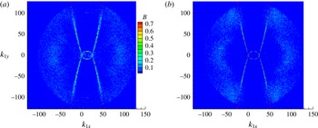
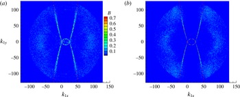
Plots of
 $B(\boldsymbol{k}_{1})$
for fixed
 $\boldsymbol{k}=(25,0)$
at (a) a higher level of nonlinearity (with
 $\hat{P}\approx 9.5\times 10^{-7}$
and
 $\unicode[STIX]{x1D6FC}\approx -4.25$
) and (b) a lower level of nonlinearity (
 $\hat{P}\approx 2.8\times 10^{-7}$
and
 $\unicode[STIX]{x1D6FC}\approx -4.6$
), where
 $\hat{P}$
is a non-dimensionalized energy flux (Pan & Yue Reference Pan and Yue2014). The time average is obtained over
 $200T_{p}$
, with
 $T_{p}$
being the modal period at the spectral peak
 $k=16$
. The vectors
 $\boldsymbol{k}_{1}$
corresponding to the exact resonance condition are indicated by – – –. The middle ellipse represents the triads of
 $\langle \unicode[STIX]{x1D702}^{\ast }(\boldsymbol{k},t)\unicode[STIX]{x1D702}(\boldsymbol{k}_{1},t)\unicode[STIX]{x1D702}(\boldsymbol{k}_{2},t)\rangle _{t}$
(
 $\unicode[STIX]{x1D714}_{k}-\unicode[STIX]{x1D714}_{1}-\unicode[STIX]{x1D714}_{2}=0$
), and the left and right branches represent, due to conjugation and isotropy,
 $\langle \unicode[STIX]{x1D702}^{\ast }(\boldsymbol{k},t)\unicode[STIX]{x1D702}^{\ast }(-\boldsymbol{k}_{1},t)\unicode[STIX]{x1D702}(\boldsymbol{k}_{2},t)\rangle _{t}$
(
 $\unicode[STIX]{x1D714}_{2}-\unicode[STIX]{x1D714}_{k}-\unicode[STIX]{x1D714}_{1}=0$
) and
 $\langle \unicode[STIX]{x1D702}^{\ast }(\boldsymbol{k},t)\unicode[STIX]{x1D702}(\boldsymbol{k}_{1},t)\unicode[STIX]{x1D702}^{\ast }(-\boldsymbol{k}_{2},t)\rangle _{t}$
(
 $\unicode[STIX]{x1D714}_{1}-\unicode[STIX]{x1D714}_{k}-\unicode[STIX]{x1D714}_{2}=0$
).
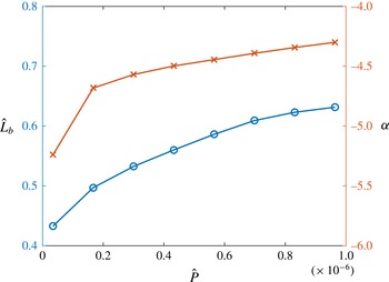
The spectral slope
 $\unicode[STIX]{x1D6FC}$
(

 $\hat{L}_{b}$
(

 $\hat{P}$
.
Data of
 $\unicode[STIX]{x1D702}(\boldsymbol{k},t)$
for the calculation of
 $B$
are drawn from the direct simulation of the primitive Euler equations (see Pan & Yue Reference Pan and Yue2014, for simulation details). At stationary stages of power-law spectra with different nonlinearity levels (measured by the energy flux
 $P$
), the discrete function
 $B(\boldsymbol{k},\boldsymbol{k}_{1})$
is evaluated using (3.1). To facilitate visualization, we fix the vector
 $\boldsymbol{k}$
without loss of generality, and plot
 $B$
as a function of
 $\boldsymbol{k}_{1}=(k_{1x},k_{1y})$
only. This is shown for two typical cases with higher and lower nonlinearity levels in figure 1(a,b) in the same finite domain, i.e. same
 $\unicode[STIX]{x0394}k$
. The discrete
 $B$
values in the
 $\boldsymbol{k}_{1}$
plane are characterized by high values in the vicinity of (but not on) curves of
 $\boldsymbol{k}_{1}$
corresponding to the exact resonance condition such as (1.2b
). Generally, these curves are given by
 $$\begin{eqnarray}\unicode[STIX]{x1D6FA}\equiv \min (|\unicode[STIX]{x1D714}_{k}-\unicode[STIX]{x1D714}_{1}-\unicode[STIX]{x1D714}_{2}|,|\unicode[STIX]{x1D714}_{1}-\unicode[STIX]{x1D714}_{k}-\unicode[STIX]{x1D714}_{2}|,|\unicode[STIX]{x1D714}_{2}-\unicode[STIX]{x1D714}_{k}-\unicode[STIX]{x1D714}_{1}|)=0.\end{eqnarray}$$
The finite width of the concentration of high values of
 $B(\boldsymbol{k}_{1})$
around the resonance curves provides a measure of the NRB. It is now evident from figure 1 that the NRB associated with higher nonlinearity level (measured by larger
 $P$
) is appreciably wider than that of lower nonlinearity level (smaller
 $P$
). We further define a quantitative measure of NRB as
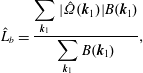 $$\begin{eqnarray}\hat{L}_{b}=\frac{\displaystyle \mathop{\sum }_{\boldsymbol{k}_{1}}|\hat{\unicode[STIX]{x1D6FA}}(\boldsymbol{k}_{1})|B(\boldsymbol{k}_{1})}{\displaystyle \mathop{\sum }_{\boldsymbol{k}_{1}}B(\boldsymbol{k}_{1})},\end{eqnarray}$$
where we have normalized (3.2) by
 $\hat{\unicode[STIX]{x1D6FA}}\equiv \unicode[STIX]{x1D6FA}/(\unicode[STIX]{x0394}kk^{1/2})$
, with
 $k=|\boldsymbol{k}|$
. As the denominator
 $\unicode[STIX]{x0394}kk^{1/2}$
estimates the frequency discreteness associated with
 $\unicode[STIX]{x0394}k$
,
 $\hat{\unicode[STIX]{x1D6FA}}$
calculates the distance of a point in the domain from the resonance curve (which can be understood as a level-set function obtaining zero on the resonance curve), measured by the number of grid spacings. With
 $\sum _{\boldsymbol{k}_{1}}$
summing all grid points of
 $\boldsymbol{k}_{1}$
, the parameter
 $\hat{L}_{b}$
measures the characteristic width of NRB by the first moment of
 $B(\boldsymbol{k}_{1})$
centred at the resonance curve.
We plot in figure 2 the variations of
 $\hat{L}_{b}$
and the resultant power-law spectral slope
 $\unicode[STIX]{x1D6FC}$
over a range of nonlinearity levels, measured by the energy flux
 $P$
. The range of nonlinearity considered here corresponds to the weak turbulence regime, where both
 $\hat{L}_{b}$
and
 $\unicode[STIX]{x1D6FC}$
increase with increase in
 $P$
. In particular, the steepened spectral slope
 $\unicode[STIX]{x1D6FC}<\unicode[STIX]{x1D6FC}_{0}$
in this range of nonlinearity is consistent with other existing experimental measurements (e.g. Wright, Budakian & Putterman Reference Wright, Budakian and Putterman1996; Brazhnikov et al.
Reference Brazhnikov, Kolmakov, Levchenko and Mezhov-Deglin2002; Denissenko et al.
Reference Denissenko, Lukaschuk and Nazarenko2007; Xia et al.
Reference Xia, Shats and Punzmann2010). This clearly marks the discrete spectrum with slope
 $\unicode[STIX]{x1D6FC}_{0}$
, associated with maximum
 $\hat{L}_{b}$
, as an upper limit in the range of weak turbulence. Physically, this is an illustration of the NRB reaching a limit with sufficient level of nonlinearity, for which the dynamics governed by quasi-resonance approximates that of exact resonance in a theoretically infinite domain. The dynamics above this limit remains elusive (e.g. Denissenko et al.
Reference Denissenko, Lukaschuk and Nazarenko2007) and is beyond our current consideration on weak turbulence.
While this study shows evidence and features of NRB, it is still desirable to develop a simple model incorporating this mechanism. We show that this can be accomplished in the framework of the KE describing the modal energy transfer due to triad interactions.
4 Quasi-resonant kinetic equation for discrete turbulence
Motivated by the insights from § 3, we develop a quasi-resonant kinetic equation (QKE) that incorporates NRB in the triad interactions. To represent such quasi-resonance, we broaden the generalized delta function (e.g. Lighthill Reference Lighthill1958) such as
 $\unicode[STIX]{x1D6FF}(\unicode[STIX]{x1D6FA}_{k12}\equiv \unicode[STIX]{x1D714}_{k}-\unicode[STIX]{x1D714}_{1}-\unicode[STIX]{x1D714}_{2})$
in (2.1c
) as a finite-width delta function of the specific form
 $$\begin{eqnarray}\unicode[STIX]{x1D6FF}(\unicode[STIX]{x1D6FA}_{k12})\sim \unicode[STIX]{x1D6FF}_{g}(\unicode[STIX]{x1D6FA}_{k12})=\frac{\unicode[STIX]{x1D6FD}}{\unicode[STIX]{x03C0}}\frac{1}{\unicode[STIX]{x1D6FD}^{2}+\unicode[STIX]{x1D6FA}_{k12}^{2}},\end{eqnarray}$$
where
 $\unicode[STIX]{x1D6FD}$
is a small parameter introduced to characterize the NRB in frequency.
The physical significance of using (4.1) can be traced back in the derivation of the KE from the Euler equations. Rigourously speaking, the delta function
 $\unicode[STIX]{x1D6FF}(\unicode[STIX]{x1D6FA}_{k12})$
in (2.1c
) is a result of the closure for the third-order cumulant
 $J_{k12}$
(
 ${\sim}$
ensemble average of multiplication of modal amplitudes at
 $\boldsymbol{k}$
,
 $\boldsymbol{k}_{1}$
and
 $\boldsymbol{k}_{2}$
), which renders
 $J_{k12}$
non-zero only when
 $\unicode[STIX]{x1D6FA}_{k12}=0$
. The treatment of (4.1) broadens the non-zero region of
 $J_{k12}$
, and, in the framework of the QKE, effectively allows the triads in quasi-resonance to be excited for nonlinear energy transfer. The specific form (4.1) of the finite-width delta function is used as it is mathematically a direct result in the derivation of the closure, by relaxing the limit of zero-approaching small parameter (to account for the discrete wavenumbers) in the application of the Sokhotski–Plemelj theorem (cf. Zakharov et al.
Reference Zakharov, L’vov and Falkovich1992). Therefore, this form of (4.1) is more than an approximation, but also a theoretical model for discrete turbulence.
We further define the normalized NRB,
 $$\begin{eqnarray}\unicode[STIX]{x1D705}=\frac{\unicode[STIX]{x1D6FD}}{\unicode[STIX]{x0394}kk^{1/2}}.\end{eqnarray}$$
With
 $\unicode[STIX]{x0394}kk^{1/2}$
measuring the frequency discreteness associated with
 $\unicode[STIX]{x0394}k$
at wavenumber
 $k$
, the non-dimensional parameter
 $\unicode[STIX]{x1D705}$
characterizes the ratio between NRB and grid spacing, i.e. the number of grid points underneath the broadening. In a single simulation corresponding to a certain nonlinearity level,
 $\unicode[STIX]{x1D705}$
is set as a constant, and
 $\unicode[STIX]{x1D6FD}$
is calculated accordingly as a function of
 $k$
and
 $\unicode[STIX]{x0394}k$
. This ensures that the NRB scales with the discreteness, and is evenly applied, at all wavenumbers. (Specifically, near the resonance manifold defined by (1.2), a similar number of discrete modes is excited at each wavenumber scale.)
The wavenumber in the simulation spans a discrete two-dimensional space of
 $k_{x}\times k_{y}\in [\unicode[STIX]{x0394}k,k_{max}]\times [\unicode[STIX]{x0394}k,k_{max}]$
, with increment
 $\unicode[STIX]{x0394}k$
in both
 $k_{x}$
and
 $k_{y}$
. We assume that all energy transfer to
 $k>k_{max}$
is dissipated. This can be accomplished by adding an additional term to the quasi-resonant form of (2.1a
), given by
 $$\begin{eqnarray}\unicode[STIX]{x1D6E4}(n_{k})=-\iint _{k_{max}<k_{1}<k_{d}}8\unicode[STIX]{x03C0}|V_{\boldsymbol{k}_{1}\boldsymbol{k}\boldsymbol{k}_{2}}|^{2}\unicode[STIX]{x1D6FF}(\boldsymbol{k}_{1}-\boldsymbol{k}-\boldsymbol{k}_{2})\unicode[STIX]{x1D6FF}_{g}(\unicode[STIX]{x1D714}_{k_{1}}-\unicode[STIX]{x1D714}_{k}-\unicode[STIX]{x1D714}_{k_{2}})n_{k}n_{k_{2}}\,\text{d}\boldsymbol{k}_{1}\,\text{d}\boldsymbol{k}_{2},\end{eqnarray}$$
which selects all triads transferring energy from
 $k\in [\unicode[STIX]{x0394}k,k_{max}]$
to
 $[k_{max},k_{d}]$
. While
 $n(k>k_{max})$
is set to be zero and not updated in the simulation,
 $[k_{max},k_{d}]$
serves as an energy sink regime, which physically absorbs energy transferred from
 $[\unicode[STIX]{x0394}k,k_{max}]$
. In theory,
 $k_{d}=2k_{max}$
accounts for all such triads, and (4.3) provides a parameter-free dissipation model, with
 $\unicode[STIX]{x1D6E4}(n_{k})$
representing the decreasing rate of
 $n_{k}$
due to energy transfer to the dissipation regime above
 $k_{max}$
. The energy flux can be directly evaluated as the energy transfer across
 $k_{max}$
,
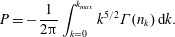 $$\begin{eqnarray}P=-\frac{1}{2\unicode[STIX]{x03C0}}\int _{k=0}^{k_{max}}k^{5/2}\unicode[STIX]{x1D6E4}(n_{k})\,\text{d}k.\end{eqnarray}$$
To obtain a stationary spectrum, a large-scale forcing is required. Instead of adding an extra forcing term (e.g. Pushkarev, Resio & Zakharov Reference Pushkarev, Resio and Zakharov2003), we assume that the forcing exactly compensates for the decrease of
 $n(k)$
at large forcing scales due to energy transfer to small scales, i.e. we numerically keep
 $n(k)$
in the forcing regime unchanged in the simulation. This approach is found to be effective in obtaining the converged stationary spectrum.
The configuration of the QKE to study discrete capillary-wave turbulence is now complete. Starting with a somewhat arbitrary initial spectrum
 $n_{I}(k)$
, we numerically evolve the spectrum in time according to (2.1) and (4.1)–(4.3) (with all integrals calculated as summations on discrete grid points), with a second-order Runge–Kutta scheme. The simulations are run for sufficient time until a stationary spectrum is established.
5 Predictions of the QKE
We perform systematic numerical simulations of the QKE by varying the values of
 $\unicode[STIX]{x1D705}$
and
 $\unicode[STIX]{x0394}k$
. In each simulation, without loss of generality, we use an initial spectrum
 $n_{I}(k)=\exp (-k^{2}/5)$
, maximum wavenumber
 $k_{max}=32$
, and forcing on the fundamental wavenumber
 $k_{f}=\unicode[STIX]{x0394}k$
.
We first consider the evolutions of the spectra governed by the QKE with different values of
 $\unicode[STIX]{x1D705}$
for fixed
 $\unicode[STIX]{x0394}k~(=1)$
. After sufficient time, the initial spectrum evolves to a stationary state corresponding to power-law solutions with different spectral slopes
 $\unicode[STIX]{x1D6FC}$
for different values of
 $\unicode[STIX]{x1D705}$
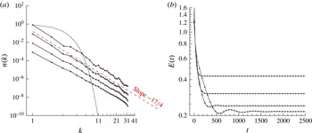
. These are plotted in figure 3(a) for select values of
 $\unicode[STIX]{x1D705}$
. The evolutions of the total spectral energy
 $E\equiv \int _{\boldsymbol{k}}n(k)k^{5/2}\,\text{d}k/(2\unicode[STIX]{x03C0})$
for these cases are plotted in figure 3(b), showing that the stationary state is reached as the power-law spectrum is formed.
(a) Converged stationary power-law spectra at
 $t=2500$
and (b) variation of the total energy
 $E$
in the spectral evolutions for
 $\unicode[STIX]{x1D705}=0.01$
(

 $\unicode[STIX]{x1D705}=0.02$
(

 $\unicode[STIX]{x1D705}=0.04$
(

 $\unicode[STIX]{x1D705}=0.1$
(

 $\unicode[STIX]{x0394}k=1$
. In (a), the initial spectrum (— ⋅ —) is plotted and the theoretical slope
 $\unicode[STIX]{x1D6FC}_{0}=-17/4$
(– – –) is indicated. Curves with different values of
 $\unicode[STIX]{x1D705}$
are shifted for clarity.
The evaluation of the spectral slope
 $\unicode[STIX]{x1D6FC}$
is straightforward at the stationary state. With
 $\unicode[STIX]{x1D6FC}$
obtained, the Kolmogorov constant
 $C=\langle n(k)/(2\unicode[STIX]{x03C0}P^{1/2}k^{\unicode[STIX]{x1D6FC}})\rangle _{k}$
is calculated, where
 $P$
is from (4.4) and
 $\langle \rangle _{k}$
denotes the average over the range of
 $k$
. We note that this calculation of
 $C$
provides a measure of the energy cascade capacity of a spectrum with uncertain slope
 $\unicode[STIX]{x1D6FC}$
. (In specificity, a spectrum associated with larger
 $C$
has smaller energy flux scaled by the spectral amplitude
 $n(k)/k^{\unicode[STIX]{x1D6FC}}$
, i.e. weaker capacity of transferring energy.)
Guided by the analysis in § 3, we are particularly interested in the existence of a value
 $\unicode[STIX]{x1D705}=\unicode[STIX]{x1D705}_{0}$
where both
 $\unicode[STIX]{x1D6FC}$
and
 $C$
attain their values for a continuous spectrum of
 $\unicode[STIX]{x1D6FC}=\unicode[STIX]{x1D6FC}_{0}=-17/4$
and
 $C=C_{0}=6.97$
associated with maximum energy transfer. Cases with
 $\unicode[STIX]{x1D705}<\unicode[STIX]{x1D705}_{0}$
then correspond to discrete turbulence with insufficient NRB, as a manifestation of the finite box effect. With these considerations, values of
 $\unicode[STIX]{x1D6FC}$
and
 $C$
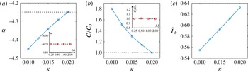
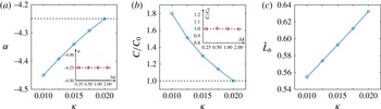
are plotted in figure 4(a,b) for varying
 $\unicode[STIX]{x1D705}$
(again with fixed
 $\unicode[STIX]{x0394}k$
). It is shown that the theoretical values of
 $\unicode[STIX]{x1D6FC}_{0}$
and
 $C_{0}$
are simultaneously achieved at
 $\unicode[STIX]{x1D705}=\unicode[STIX]{x1D705}_{0}\approx 0.02$
by discrete turbulence. This thus physically corresponds to an upper limit, in our consideration of NRB, for which the dynamics excited by the quasi-resonant interactions approximates that of the exact resonance in a theoretically infinite domain. For
 $\unicode[STIX]{x1D705}<\unicode[STIX]{x1D705}_{0}$
, the plots show that
 $\unicode[STIX]{x1D6FC}<\unicode[STIX]{x1D6FC}_{0}$
and
 $C>C_{0}$
are monotonically obtained with the decrease of
 $\unicode[STIX]{x1D705}$
in the considered range. These results are clear illustrations of physics with insufficient nonlinearity level (in a finite domain), i.e. steepened spectral slope and reduced capacity of energy cascade. These phenomena are completely consistent with the direct simulation of the primitive Euler equations (Pan & Yue Reference Pan and Yue2014) and experiments (e.g. Denissenko et al.
Reference Denissenko, Lukaschuk and Nazarenko2007; Deike et al.
Reference Deike, Bacri and Falcon2013).
The effects of
 $\unicode[STIX]{x0394}k$
on
 $\unicode[STIX]{x1D6FC}$
and
 $C$
are plotted in the two insets of figure 4(a,b), using the case with
 $\unicode[STIX]{x1D705}=\unicode[STIX]{x1D705}_{0}$
as a representation. It is clear that both
 $\unicode[STIX]{x1D6FC}$
and
 $C$
are independent of
 $\unicode[STIX]{x0394}k$
and functions of
 $\unicode[STIX]{x1D705}$
only. Hence, the parameter
 $\unicode[STIX]{x1D705}$
, as introduced in the QKE, is the only parameter governing the stationary spectrum of discrete turbulence. The absence of dependence on
 $\unicode[STIX]{x0394}k$
can be expected from the scale invariance of the QKE and its associated power-law solution (as varying
 $\unicode[STIX]{x0394}k$
is equivalent to extending the same power-law spectrum, by scaling). The physical implication of the absence of dependence on
 $\unicode[STIX]{x0394}k$
is profound. It signifies that values of
 $\unicode[STIX]{x1D6FC}$
and
 $C$
, both reflections of dynamics of energy transfer on a discrete grid, are solely determined by the ratio between NRB and grid discreteness, i.e. the same dynamics can be obtained with different NRB and grid discreteness, provided that the ratio of the two is maintained.
Plots of (a)
 $\unicode[STIX]{x1D6FC}$
, (b)
 $C/C_{0}$
(with
 $C_{0}=6.97$
) and (c)
 $\hat{L}_{b}$
(associated with the same
 $\unicode[STIX]{x1D6FC}$
) as functions of
 $\unicode[STIX]{x1D705}$
for
 $\unicode[STIX]{x0394}k=1$
. Insets: (a)
 $\unicode[STIX]{x1D6FC}$
and (b)
 $C/C_{0}$
as functions of
 $\unicode[STIX]{x0394}k$
for
 $\unicode[STIX]{x1D705}=\unicode[STIX]{x1D705}_{0}$
. The theoretical values (– – –) of
 $\unicode[STIX]{x1D6FC}_{0}=-17/4$
and
 $C/C_{0}=1$
are indicated in (a) and (b), and their insets.
To corroborate the formulation of
 $\unicode[STIX]{x1D705}$
in the QKE using the results from the Euler equations in § 3, we plot
 $\hat{L}_{b}$
as a function of
 $\unicode[STIX]{x1D705}$
associated with the same spectral slope
 $\unicode[STIX]{x1D6FC}$
in figure 4(c). It is clear that
 $\hat{L}_{b}$
increases monotonically with
 $\unicode[STIX]{x1D705}$
, with the correlation being linear in the considered range. This result provides a direct justification of the QKE and further confirms the point that the influence of the nonlinearity level on the spectral properties, as observed in Euler equation simulations, can be explained through the NRB.
6 Conclusion
We study discrete capillary-wave turbulence in a finite domain. Using direct simulations of the Euler equations, we analyse and elucidate the role of nonlinear resonance broadening (NRB) in the stationary power-law spectrum in discrete turbulence. Motivated by this insight, we propose a simple model describing discrete wave turbulence in the framework of the kinetic equation (KE). Under the assumption of a theoretically infinite domain, the KE yields a stationary solution of a continuous power-law spectrum with slope
 $\unicode[STIX]{x1D6FC}_{0}=-17/4$
and Kolmogorov constant
 $C_{0}=6.97$
(corrected from the original work), corresponding to an upper bound of energy flux in the limit of continuous wavenumber. We generalize this framework to a quasi-resonant kinetic equation (QKE) applicable to discrete wavenumber
 $\unicode[STIX]{x0394}k$
in a finite domain. We show that the QKE can be parameterized by a single parameter
 $\unicode[STIX]{x1D705}$
expressing the ratio of NRB to wavenumber discreteness. At
 $\unicode[STIX]{x1D705}=\unicode[STIX]{x1D705}_{0}\approx 0.02$
, the theoretical values of
 $\unicode[STIX]{x1D6FC}_{0}$
and (the corrected)
 $C_{0}$
are simultaneously recovered, corresponding physically to sufficient NRB for a given
 $\unicode[STIX]{x0394}k$
, or sufficiently small
 $\unicode[STIX]{x0394}k$
for a given nonlinearity. For
 $\unicode[STIX]{x1D705}<\unicode[STIX]{x1D705}_{0}$
, the simulation results replicate those with insufficient nonlinearity level, namely steepened spectral slope
 $\unicode[STIX]{x1D6FC}<\unicode[STIX]{x1D6FC}_{0}$
and reduced capacity of energy cascade
 $C>C_{0}$
. The form of the parameter
 $\unicode[STIX]{x1D705}$
and its effect on the spectral properties corroborate results from simulations of primitive Euler equations at different nonlinearity levels. The elucidation of the role of NRB in discrete turbulence and the framework of the QKE are expected to be valid for weak turbulence in other physical contexts.