1. Introduction

Computer simulation models are now essential tools in many scientific fields, and a rapidly expanding philosophical literature examines a host of accompanying methodological and epistemological questions about their roles and uses (e.g., Frigg and Reiss Reference Frigg and Reiss2009; Grüne-Yanoff and Weirich Reference Grüne-Yanoff and Weirich2010; Winsberg Reference Winsberg2010, Reference Winsberg and Zalta2018; Weisberg Reference Weisberg2013; Parke Reference Parke2014; Jebeile Reference Jebeile2017; Beisbart and Saam Reference Beisbart and Saam2019). Climate science is one such field (Edwards Reference Edwards, Miller and Edwards2001), and questions about the interpretation and reliability of the simulation models used to understand, attribute, and predict climate change have received considerable attention (e.g., Lloyd Reference Lloyd2010, Reference Lloyd2015; Oreskes, Stainforth, and Smith Reference Oreskes, Stainforth and Smith2010; Parker Reference Parker2011, Reference Parker2013; Petersen Reference Petersen2012; Frigg, Smith, and Stainforth Reference Frigg, Smith and Stainforth2013, Reference Frigg, Smith and Stainforth2015; Steele and Werndl Reference Steele and Werndl2016; Thompson, Frigg, and Helgeson Reference Thompson, Frigg and Helgeson2016; Vezér Reference Vezér2016; Lloyd and Winsberg Reference Lloyd and Winsberg2018).

One conspicuous feature of scientific discourse about the simulation models used in climate science, and in environmental modeling more broadly, is the attention given to where a model lies on a spectrum from simple to complex (e.g., McGuffie and Henderson-Sellers Reference McGuffie and Henderson-Sellers2001; Jakeman, Letcher, and Norton Reference Jakeman, Letcher and Norton2006; Smith et al. Reference Smith, Palmer, Purves, Vanderwel, Lyutsarev, Calderhead, Joppa, Bishop and Emmott2014). While this attention to model complexity has informed some of the philosophical discourse on simulation modeling (e.g., Parker Reference Parker2010), its relevance for the literature on simplicity in science remains largely unexplored.

This literature on simplicity addresses whether and why simpler theories (or hypotheses, models, etc.) might be—other things being equal—better than complex ones. Different ways of unpacking “simpler” and “better”? yield a diversity of specific theses, with correspondingly different justifications (see Sober [Reference Sober2015] and Baker [Reference Baker and Zalta2016], for details and history). A number of distinctly modern variants rest on mathematical theorems tying well-defined notions of simplicity to benefits such as predictive accuracy (Akaike Reference Akaike, Petrov and Csaki1973; Forster and Sober Reference Forster and Sober1994), reliability (Vapnik Reference Vapnik1998; Harman and Kulkarni Reference Harman and Kulkarni2007), and efficient inquiry (Kelly Reference Kelly2004, Reference Kelly2007). Arguably more domain-specific appeals to parsimony include instances in phylogenetics (see Sober Reference Sober1988, Reference Sober2015) and animal cognition (Sober Reference Sober and Lurz2009, Reference Sober2015; Clatterbuck Reference Clatterbuck2015).

Here we discuss a notion of simplicity drawn from scientific discourse on environmental simulation modeling and expound its importance in the context of climate risk management. The new idea that we bring to the simplicity literature is that simplicity benefits the assessment of uncertainty in the model's predictions. The short explanation for this is that quantifying uncertainty in the predictions of computer simulation models requires running the model many times over using different inputs, and simpler models enable this because they use less computer processor time. (The quantification of uncertainty in light of present knowledge and available data should be clearly distinguished from the reduction of uncertainty that may occur as knowledge and data accumulate over time. We address the former, not the latter.)

While complexity obstructs uncertainty quantification, complex models may behave more like the real-world system, especially when pushed into Anthropocene conditions. So there is a trade-off between a model's capacity to realistically represent the system and its capacity to tell us how confident it is in its predictions. Both are desirable from a purely scientific or epistemic perspective as well as for their contributions to the model's utility in climate risk management. Whether simpler is better in any given case depends on details that go beyond the scope of this article, but the critical importance of uncertainty assessment for addressing climate risks (e.g., Reilly et al. Reference Reilly, Stone, Forest, Webster, Jacoby and Prinn2001; Smith and Stern Reference Smith and Stern2011) is why simpler models can be epistemically better for informing decisions.

In what follows, we introduce the relevant notion of simplicity and a way to measure it (sec. 2). We then explain the link from simplicity to uncertainty quantification (sec. 3), arguing that through this link, simplicity becomes epistemically relevant to model choice and model development (sec. 4). We next briefly discuss the resulting trade-off, highlighting the roles of nonepistemic values and high-impact, low-probability outcomes in mediating the importance of uncertainty assessment for climate risk management (sec. 5).

2. Simplicity and Run Time

Environmental simulation models populate a spectrum from simple to complex, and attention to a model's position on this spectrum is a pervasive feature of both published research and everyday scientific discourse. All computational models idealize their target systems by neglecting less important processes and by discretizing space and time. What makes a model comparatively complex is the explicit representation of more processes and feedback thought to operate in the real-world system or greater resolution in the discretization (i.e., smaller grid size or a shorter time step). Greater complexity can allow for a more realistic depiction of the target system, while simpler models must work with a more idealized picture.

Realistic depictions can provide benefits but come at a cost: complex models demand more computer processor time. Here we use the length of time needed to run the simulation model on a computer, or the model's run time, as a proxy for model complexity. (To begin, suppose the model runs on a single processor; we discuss parallel computing further below.) Run time is, of course, a processor-dependent measure: a faster computer processor can run the same program in less time. But this will not hamper our discussion since we are ultimately concerned with between-model comparisons that can be relativized to fixed hardware without loss of import.Footnote ¹ Moreover, differences in processor speed are in practice relatively small (in the neighborhood of times two for processors in service at any given time) when compared with differences in run time across models (factors of tens to trillions). Run time also depends on the time span simulated, but this, too, is something we can hold constant across models in order to compare apples to apples.

Another feature of run time as a measure of simplicity is that it applies to models understood in the most concrete sense. Run time is not a feature of calculations understood abstractly but of a specific piece of computer code written in a specific programming language (and run on a specific machine). A consequence of this is that two pieces of code with meaningfully different run times can instantiate what is, in some sense, the same model. What that means for our discussion is that the trade-off we examine applies most unyieldingly to computationally efficient programming; inefficiently coded models can, to a point, be sped up without sacrificing realism.

Run time can be contrasted with other concepts already implicated in discussions of simplicity's role in science, for example, the number of adjustable parameters in a hypothesis. Run time quantifies the amount of calculating needed to use the model, while the number of parameters concerns the model's plasticity in the face of observations. Simulation models contain adjustable parameters, but their number is often poorly defined, since quantities appearing in the computer code might be fixed in advance for one application but allowed to vary in the next.Footnote ²

To make the discussion more concrete (and point readers to further details), we introduce a small collection of models that together illustrate the simplicity-complexity spectrum in environmental simulation modeling. We choose from models that have been used to investigate the contribution to sea level rise from the Antarctic ice sheet (AIS), a key source of uncertainty about future sea level rise on time scales of decades to centuries (DeConto and Pollard Reference DeConto and Pollard2016; Bakker, Louchard, and Keller Reference Bakker, Louchard and Keller2017; Bakker, Wong, et al. Reference Bakker, Wong, Ruckert and Keller2017).

The Danish Antarctic Ice Sheet model (DAIS; Shaffer Reference Shaffer2014; Ruckert et al. Reference Ruckert, Shaffer, Pollard, Guan, Wong, Forest and Keller2017) is the simplest of four models we consider here. It represents the AIS as a perfect half spheroid resting on a shallow cone of land—a highly aggregate representation in the sense that just a few numbers summarize a vast and varied landscape (the AIS is larger than the United States). DAIS represents several key processes governing ice mass balance, including snow accumulation and melting at contact surfaces with air, water, and land.

The Building Blocks for Relevant Ice and Climate Knowledge model (BRICK; Bakker, Wong, et al. Reference Wong and Keller2017; Wong, Bakker, Ruckert, et al. Reference Wong, Bakker, Ruckert, Applegate, Slangen and Keller2017) couples a slightly expanded version of DAIS with similarly aggregate models of global atmosphere and ocean temperature, thermal expansion of ocean water, and contributions to sea level from other land ice (glaciers and the Greenland ice sheet). Compared to DAIS, BRICK represents an additional AIS process (marine ice sheet instability), as well as a number of interactions with other elements of the global climate system, including feedback between sea level change and AIS behavior.

The Pennsylvania State University 3-D ice sheet-shelf model (PSU3D; Pollard and DeConto Reference Pollard and DeConto2012; DeConto and Pollard Reference DeConto and Pollard2016) includes fewer global-scale interconnections than BRICK but a much richer representation of both AIS processes and local ocean and atmosphere interactions. PSU3D is a spatially resolved model of AIS in the sense that spatial variation in ice thickness and underlying topography are explicitly represented and incorporated into AIS dynamics. PSU3D represents many additional AIS processes (beyond DAIS), including ice flow through deformation and sliding, marine ice cliff instability, and ice shelf calving.

The last and most complex model we use to illustrate the simplicity spectrum is the Community Earth System Model (CESM; Hurrell et al. Reference Hurrell2013; Lipscomb and Sacks Reference Lipscomb and Sacks2013; Lenaerts et al. Reference Lenaerts, Vizcaino, Fyke, Kampenhout and van den Broeke2016), incorporating spatially resolved atmosphere, ocean, land surface, and sea ice components and allowing global ocean and atmosphere circulation to interact with the AIS. While dynamic (two-way) coupling of CESM with a full AIS model is still under development (Lipscomb Reference Lipscomb2017, Reference Lipscomb2018), recent work (Lenaerts et al. Reference Lenaerts, Vizcaino, Fyke, Kampenhout and van den Broeke2016) uses a static ice sheet surface topography to investigate one aspect of future AIS dynamics, the surface mass balance (net change in ice mass due to precipitation, sublimation, and surface melt).

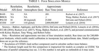
The resolution and run time of the models described above are provided in table 1. Figure 1 summarizes and illustrates the models with special attention to key differences in complexity that account for their different run times.

Table 1.

Four Simulation Models

Model	Resolution, AIS (km)	Resolution, Atmosphere (km)	Approximate Run Time (min)	Reference
DAIS	NA	NA	.001	Ruckert et al. (Reference Ruckert, Shaffer, Pollard, Guan, Wong, Forest and Keller2017)
BRICK	NA	NA	.1	Wong, Bakker, Ruckert, et al. (2017)
PSU3D	10	40 (regional)	25,000	DeConto and Pollard (Reference DeConto and Pollard2016)
CESM	110∗	110 (global)	2,000,000,000†	Lenaerts et al. (Reference Lenaerts, Vizcaino, Fyke, Kampenhout and van den Broeke2016)

Sources.—Bakker, Applegate, and Keller (Reference Bakker, Applegate and Keller2016), DeConto and Pollard (Reference DeConto and Pollard2016), Lenaerts et al. (Reference Lenaerts, Vizcaino, Fyke, Kampenhout and van den Broeke2016), UCAR (2016), Ruckert et al. (Reference Ruckert, Shaffer, Pollard, Guan, Wong, Forest and Keller2017), Wong, Bakker, Ruckert, et al. (Reference Wong, Bakker, Ruckert, Applegate, Slangen and Keller2017), and personal communication with Kelsey Ruckert, Tony Wong, and Robert Fuller.

Note. Resolution and approximate run time of four simulation models. Run times are for 240,000-year hindcasts, which enable model calibration to incorporate key paleoclimate data. Model configurations are as per the reference.

∗ Resolution of CESM's land surface component used to calculate surface mass balance.

^† The hindcast length used for this comparison is impractical for models as complex as CESM. Yet because of parallel computing (see sec. 3.1) this number is not quite as outlandish as it may seem.

Figure 1.

Four environmental simulation models discussed in the text. Based on configurations of DAIS, BRICK, PSU3D, and CESM in Ruckert et al. (Reference Ruckert, Shaffer, Pollard, Guan, Wong, Forest and Keller2017), Wong, Bakker, Ruckert, et al. (2017), DeConto and Pollard (Reference DeConto and Pollard2016) (Pliocene simulation), and Lenaerts et al. (Reference Lenaerts, Vizcaino, Fyke, Kampenhout and van den Broeke2016), respectively. Different configurations of the same model may correspond to somewhat different depictions within the visual schema used here. CESM includes many additional system components not pictured.

3. Epistemic Relevance for Model Choice

Having introduced a notion of simplicity and a way to measure it, we now turn to the benefits enabled by this kind of simplicity. The proximate consequence of using a simpler model is that a shorter run time allows for more model runs. That, in turn, has consequences for what one can learn from the model. But we begin with the proximate step.

Given a computing budget of some number of processor-hours, a simple calculation of computing budget divided by run time yields a theoretical maximum for the number of times the model can be run. Figure 2a displays this reciprocal relationship for two example computing budgets. Each point along such a curve corresponds to a different model choice: moving from left to right, one trades away model complexity (run time) in exchange for more runs. (Because such plots become hard to read with larger numbers, it will be helpful to use a logarithmic scale on the axes; we introduce this visualization in fig. 2b.)

Figure 2.

a, Two computing budgets, illustrating the reciprocal relationship between run time and number of runs. Arrows illustrate how to read the figure: a model that runs in 1 hour (e.g.) can be run 24 times on a 1-day budget and 120 times on a 5-day budget. b, Same figure, now plotted on logarithmic axes for a wider view (we use this format to accommodate very large and very small numbers in one plot).

As per figure 2, run time and a computing budget determine how many model runs can be carried out. This run limit in turn constrains what methods can be employed at key stages of a modeling study, including calibration and projection. Model calibration is a process of tuning, weighting, or otherwise constraining the values of adjustable parameters in order to make the model the best representation that it can be of the system under study. Subsequent projection involves running the calibrated model into the future to see what it foretells, conditional on assumptions about how required exogenous (supplied from outside the model) inputs will play out over the time frame in question.Footnote ³ We discuss calibration and projection in turn, in each case detailing how the feasible number of model runs constrains the approach taken to these modeling tasks and what those constraints mean for the quantification of uncertainty.

3.1. Calibration

In the geosciences, model calibration typically aims to exploit both fit with data and prior knowledge about parameters (which often have a physical interpretation; see, e.g., Pollard and DeConto Reference Pollard and DeConto2012; Shaffer Reference Shaffer2014). How this is done varies, and some methods require more model runs than others. To illustrate the dependence between model simplicity and calibration methods, we contrast three methods that together span the runs-required gamut. At one extreme lies Markov Chain Monte Carlo (MCMC), the gold standard in Bayesian model calibration (Bayesian inference is a natural fit for the task of integrating observations with prior knowledge). Near the middle is an approach called (somewhat confusingly) precalibration.Footnote ⁴ At the other extreme lies hand tuning. We describe each below.

For the following discussion, assume a model that is deterministic and at each time step calculates the next system state as a function of the current state plus exogenous inputs (also called forcings) impinging on the system. Assume a set of historical observations, both of the forcings and of quantities corresponding to the model's state variables. Finally, assume a measure of fit between the time series of observations and the corresponding series of values produced by the model when driven by historical forcings (a hindcast).

Bayesian calibration begins with a prior probability distribution over all parameter combinations (the model's parameter space) and updates that prior in light of observations to arrive at a posterior distribution. In principle, the updating takes into account fit between those observations and every possible version of the model (every combination of parameter values). The posterior can therefore be calculated exactly (analytically) only where a suitably tractable mathematical formula maps parameter choices to hindcast-observation fit (the likelihood function). This is not the case for computer simulation models, where fit can be assessed only by running the simulation and comparing the resulting hindcast with the observations. In this case, the posterior can still be approximated numerically, but this requires evaluating fit with observations (running the model each time) for a very large number of parameter choices. MCMC is a standard approach to numerically approximating Bayesian posterior distributions and requires tens of thousands to millions of model runs to implement (Metropolis et al. Reference Metropolis, Rosenbluth, Rosenbluth, Teller and Teller1953; Kennedy and O—Hagan Reference Kennedy and O’Hagan2001; van Ravenzwaaij, Cassey, and Brown Reference van Ravenzwaaij, Cassey and Brown2018; for application to ice sheet modeling, see Bakker, Applegate, and Keller [Reference Bakker, Applegate and Keller2016] and Ruckert et al. [Reference Ruckert, Shaffer, Pollard, Guan, Wong, Forest and Keller2017]).

In contrast to MCMC's thorough survey of parameter space, precalibration involves running the model at a smaller number of strategically sampled parameter-value combinations (e.g., 250, 1,000, and 2,000, in Sriver et al. [Reference Sriver, Urban, Olson and Keller2012], Ruckert et al. [Reference Ruckert, Shaffer, Pollard, Guan, Wong, Forest and Keller2017], and Edwards et al. [Reference Edwards, Cameron and Rougier2011], respectively). Each of the resulting hindcasts is compared against observations using a streamlined, binary standard of fit'sorting the hindcasts into two classes: those reasonably similar to the observations and those not. The result is a dichotomous characterization of parameter choices as plausible or implausible, the latter unsuitable for use in projection.

The third method we highlight, hand tuning, encompasses a diverse set of practices that share some common features including varying parameters one at a time rather than jointly, using different approaches to model-observation fit (or different observations altogether) for different parameters, calibrating submodel components separately, a greater emphasis on expert assessment of parameter values, and a goal of identifying a single best parameter choice (for at least a majority of the parameters, sometimes for all). Hand tuning may not be clearly separated from model development, tends to be less transparent than the previous two approaches, and examines overall model behavior (and model-observation fit) for a relatively small number of parameter choices (very roughly, less than 100). Examples include Scheller et al. (Reference Scheller, Domingo, Sturtevant, Williams, Rudy, Gustafson and Mladenoff2007) and Pollard and DeConto (Reference Pollard and DeConto2012); calibration of general circulation models (Meehl et al. Reference Meehl, Covey, Delworth, Latif, McAvaney, Mitchell, Stouffer and Taylor2007) and earth system models such as CESM also generally falls into this category (Hourdin et al. Reference Hourdin2017).

To summarize key points for current purposes, hand tuning samples the smallest number of possible parameter choices and aims to identify the best among them. Precalibration examines (on the order of) 100 times more parameter choices and issues a dichotomous division of those into the plausible and implausible. MCMC examines (roughly) 1,000 times more than that and exhaustively quantifies the relative plausibility of every possible parameter choice in the form of a probability distribution. Methods that demand more model runs do more to characterize uncertainty about parameter choices, both by testing more possible values for the parameters and by furnishing a richer characterization of uncertainty about those values.

By limiting the feasible number of runs, model complexity undermines the characterization of parameter uncertainty. Figure 3 illustrates this point using the models from section 2 and two example computing budgets. The lower diagonal line shows a 10-day budget (240 processor-hours). For researchers working on a single processor, this is a plausible limit on the computing time that can realistically be devoted to model calibration (in part since the calibration procedure might be repeated three to five times in the course of troubleshooting and replicating results). Points on or below this line are feasible on a 240 processor-hour budget. The figure shows that on this budget, DAIS can be calibrated by MCMC and BRICK by precalibration; PSU3D and CESM cannot be calibrated by any means.

Figure 3.

Example computing budgets compared with approximate run times for four simulation models (see table 1). Left boundaries of the shaded columns show approximate minimum run requirements for calibration methods discussed in the text (supposing ∼10 parameters are calibrated). The region below a computing-budget diagonal shows which calibration methods are feasible for each model on that budget. Expands on Bakker, Applegate, and Keller (Reference Bakker, Applegate and Keller2016).

With access to a high-performance computing cluster, much larger computing budgets can be contemplated: 400,000 processor-hours is a routine high-performance computing allocation in 2019 for research supported by awards from the US National Science Foundation (UCAR 2019). Since 400,000 hours would occupy a single processor for 46 years, such a budget can be properly exploited only where the computing workload can be parallelized (split between multiple processors that run in parallel). Spread over 1,000 processors, 400,000 hours lasts a little over 2 weeks. While precalibration is easily parallelized, the most widely used algorithm for implementing MCMC (Metropolis et al. Reference Metropolis, Rosenbluth, Rosenbluth, Teller and Teller1953; Robert and Casella Reference Robert and Casella1999) requires that model runs be executed serially. There are, however, a number of kindred approaches to numerically approximating a Bayesian posterior, some of which can be substantially parallelized (Lee et al. Reference Lee, Huran, Fuller, Pollard and Keller2020, and references therein).

The upper diagonal in figure 3 shows a 400,000-hour budget. With those resources, BRICK can easily be calibrated by numerical Bayesian methods, and PSU3D moves to the edge of precalibration territory. A single hindcast using CESM is still well out of reach. Parallelization and large computing clusters substantially shift the goalposts, but they cannot dissolve the fundamental trade-off between model complexity and uncertainty quantification.

4. Epistemic and Nonepistemic Benefits

We have argued that simplicity, measured via run time, is epistemically relevant to model choice. But some readers may be drawn to another framing of the issue, on which the value of this kind of simplicity is in fact not epistemic but merely practical (and therefore outside the traditional focus of the simplicity literature). After all, it would seem that however complex the model, projection uncertainties could be thoroughly characterized with enough processor time. The benefit of simplicity, then, is that it reduces the processor time needed to complete the research—which may sound like a practical matter rather than an epistemic one.

When comparing the consequences of different model choices, one must hold something else fixed in order to structure the comparison. The reasoning sketched above implicitly holds fixed the desired approach to calibration and projection (keeping the number and length of model runs the same). But you can make a different sort of comparison by holding something else fixed. We compare the consequences of model choice by holding the computing budget fixed, in which case simpler models enable different approaches to calibration and projection, resulting in better uncertainty quantification—a recognizably epistemic upshot. Which comparison gives the “right”? answer? The two results are complementary, not contradictory. Neither comparison tells the whole story; each isolates and illuminates one aspect of a bigger-picture bundle of trade-offs.Footnote ⁷

Analogous contrasting perspectives can be applied to the issue of cognitive benefits (such as ease of use), which are routinely dismissed as nonepistemic advantages of simplicity (e.g., Kelly and Mayo-Wilson Reference Kelly and Mayo-Wilson2010; Sober Reference Sober2015; Baker Reference Baker and Zalta2016). One way to reach this dismissive conclusion is to assume a fixed research plan detailing the concrete steps to be taken within a research project (analogous to fixing the desired approach to calibration and projection). On this sort of comparison, the benefit of employing a simple, easy-to-use theory rather than a complex and burdensome one appears to be getting the proposed work done faster or with less effort (a seemingly nonepistemic benefit). Yet, a different sort of comparison can be made by supposing a fixed cognitive-effort “budget,”? in which case easier use translates to more research completed and, as a result, more knowledge (or greater fulfillment of some epistemic value or other).Footnote ⁸

For comparison, it is worth noting that the benefits of other, well-discussed notions of simplicity also admit of multiple framings, where one perspective highlights an epistemic upshot and another highlights a practical one. Notions of simplicity that concern the flexibility of a model or hypothesis get their epistemic relevance as a result of viewing the choice between simple and complex models while holding fixed the quantity of data available. Akaike information criterion (AIC) scores (see Forster and Sober Reference Forster and Sober1994), for example, give advice about which statistical model will yield more accurate out-of-sample predictions after fitting to data. AIC does this by rewarding fit with data while penalizing flexibility (number of parameters). But the influence of the parameter penalty decreases as the number of data increase, so the more data one has, the less simplicity matters. This means that if we instead hold fixed the goal of some desired degree of predictive accuracy, the benefit of simplicity will now show up in the quantity of data needed to achieve that goal—or more to the point, the time and expense of obtaining those data. As before, making a different sort of comparison pivots an epistemic consideration into one more naturally viewed as nonepistemic.

The fixed-data perspective is often salient because obtaining more data can be costly, slow, or otherwise impractical (and because the division of scientific labor often divorces statistical analyses from data gathering). But developments in the nature of scientific research have made our fixed-budget perspective equally salient. The growth of scientific computing has shifted work from brains to computer processors where it is more easily quantified and tracked. The complexity of computational simulation models has shadowed the exponential growth of computing power, massively increasing the calculating required to answer even simple questions using a model. At the same time, run-hungry statistical computing methods for calibration and projection of these simulations multiply the “cognitive effort”? advantage of simpler models thousands to millions of times over, all within the scope of a single study or publishable unit of research. As a result, the trade-offs illuminated by contrasting modeling options on a fixed computing budget are now critical to a full understanding of the epistemology of simulation modeling.

5. Purpose and Values

Simplicity facilitates uncertainty quantification, but complex models can be more realistic and may behave more like the real-world system. How much complexity is the right amount? The question raises challenging scientific and technical issues requiring deep, case-by-case integration of geoscience, statistics, computing, and numerical approximation (issues that go far beyond the scope of this article). But equally important is the general qualitative point that, like other aspects of model evaluation (Parker Reference Parker2009; Haasnoot et al. Reference Haasnoot, Deursen, Guillaume, Kwakkel, Beek and Middelkoop2014; Addor and Melsen Reference Addor and Melsen2019), much depends on the purpose of the modeling exercise. Simulation modeling to improve scientific understanding, for example, may demand realism and benefit little from uncertainty quantification. Informing decisions, however, often demands attention to uncertainty (Smith and Stern Reference Smith and Stern2011; Keller and Nicholas Reference Keller and Nicholas2015; Rougier and Crucifix Reference Rougier, Crucifix, Lloyd and Winsberg2018).

Broadly speaking, risk assessment involves contemplating what outcomes might occur, how likely each is, and how bad each would be (Kaplan and Garrick Reference Kaplan and Garrick1981). These components jointly characterize the risk associated with a given course of action. Thinking in terms of probability and cost, for example, risk might be expressed as expected cost. This is not to say that risk management requires probabilities (Dessai and Hulme Reference Dessai and Hulme2004; Lempert et al. Reference Lempert2013; Weaver et al. Reference Weaver, Lempert, Brown, Hall, Revell and Sarewitz2013), only that some sense of the plausibility of different outcomes is needed to assess and manage risk (and that probability estimates are a common medium for this). Because simplicity enables the required uncertainty quantification while complexity impedes it, the simplicity-complexity dimension of model choice strongly influences a model's adequacy for the purpose of supporting decisions.

In climate risk management specifically, the importance of simplicity is magnified by the role of high-impact, low-probability outcomes. The limits that complexity places on uncertainty quantification are particularly unfavorable to estimating the chances of extreme possibilities, or what are referred to (in probability terms) as the tails of a distribution (e.g., Sriver et al. Reference Sriver, Urban, Olson and Keller2012; Wong and Keller Reference Wong and Keller2017; Lee et al. Reference Lee, Huran, Fuller, Pollard and Keller2020). But since these extreme outcomes (e.g., large or rapid sea level rise) are also the most dangerous and costly, estimating their probability can be central to managing risks, and relatively small changes to their estimated probability can have an outsize impact on risk calculations and management strategies.

A study by Wong, Bakker, and Keller (Reference Wong, Bakker and Keller2017) serves to illustrate these points. The authors use a relatively simple model of the AIS and other contributors to sea level rise (BRICK; sec. 2), allowing for rigorous quantification of parameter uncertainty via MCMC, followed by multiple large ensembles to propagate that uncertainty into local sea level rise projections for the city of New Orleans under each of several forcing (greenhouse gas concentration) scenarios. The resulting projections (plus other inputs and assumptions) allow for estimation of a site-specific, economically optimal levee height (such that building any higher costs more than the flood damage it would be expected to prevent) for each concentration scenario.

The simplicity of BRICK also enabled Wong et al. to characterize some model uncertainty by repeating the entire workflow for two different model configurations: one with and one without an additional (poorly understood but potentially important) mechanism of ice sheet behavior labeled fast dynamics (Pollard, DeConto, and Alley Reference Pollard, DeConto and Alley2015; DeConto and Pollard Reference DeConto and Pollard2016). Focusing on just one of the city's five levee rings and assuming a business-as-usual greenhouse gas scenario (RCP8.5; van Vuuren et al. Reference van Vuuren2011), the authors quantify the impact of this model uncertainty by confronting the base-case model's economically optimal levee with projections from the fast-dynamics model configuration. The result is an increase in estimated annual chance of flooding (seawater overtopping the levee) of one-half of one-tenth of a percent (from eight in 10,000 to 13 in 10,000). This seemingly small change adds $175 million in expected flood damage between now and 2100. A levee 25 centimeters higher could prevent much of that damage, with estimated net savings of $53 million.

To underline the key points of the illustration: simplicity can contribute to a model's adequacy for purpose by enabling quantification and propagation of parameter uncertainty into projections; estimation of probabilities for high-impact, low-probability outcomes; and characterization of deeper uncertainties (e.g., model structure, forcing scenario) by spelling out how alternative assumptions affect management strategies. Where complexity undermines such modeling activities, the model's adequacy for purpose suffers.

The broad-brush purpose of supporting climate risk management can be analyzed further in any particular instance to reveal specific nonepistemic concerns such as protecting livelihoods, preserving culture, and saving money and lives (Bessette et al. Reference Bessette, Mayer, Cwik, Vezér, Keller, Lempert and Tuana2017; CPRAL 2017). By judging models in light of purpose while also viewing these motivating values as a part of that purpose, the simplicity-complexity dimension of model choice can be seen as a coupled ethical-epistemic problem (Tuana Reference Tuana2013, Reference Tuana and Gundersen2017; Vezér et al. Reference Vezér, Bakker, Keller and Tuana2018) in which motivations and trade-offs encompass both epistemic and ethical values.

The prospect of ethical values motivating model choice may raise concerns about such values overstepping their proper role in science, and at this point our discussion links up with a large literature on ethical (or more broadly, nonepistemic) values in science (Douglas Reference Douglas2009; Elliott Reference Elliott2017), a portion of which addresses climate science specifically (e.g., Steele Reference Steele2012; Winsberg Reference Winsberg2012; Betz Reference Betz2013; Parker Reference Parker2014; Intemann Reference Intemann2015; Steel Reference Steel2016b). Here we can only note this connection, leaving further exploration of the topic for future work.

6. Conclusion

Discussions of simplicity's role in scientific method and reasoning have often recognized a loose notion of cognitive benefit—or benefit in terms of cognitive effort—associated with simple theories or models. Yet this aspect of simplicity has received relatively little attention in philosophy of science, either because the advantage is seen as self-evident and trivial or because the upshot is judged a matter of convenience, not epistemology.

This convenience-not-epistemology verdict is a natural consequence of the practice (common in much traditional philosophy of science) of attending to formal relationships between theory and data while idealizing away the messy human elements of science. But for today's computer simulation models, the “effort”? required to operate the model—now understood in terms of computing resources, not cognitive burden—is too consequential to neglect. Computing demands sharply constrain how a model can be used and what can be learned from it.

We have used the run time of a simulation model as a measure of the model's complexity: simple models run faster, and complex models run more slowly. The importance of run time to the epistemology of computer simulation can be seen clearly by adopting what we have called a fixed-budget perspective: compare what can be achieved with a simpler model to what can be achieved with a more complex one on the same computing budget. On such a comparison, simplicity facilitates quantification of parameter uncertainty and propagation of this and other sources of uncertainty into model projections, including estimates of chances for low-probability, high-impact outcomes.

How much one values these benefits is a further question that is tied up with the purpose of a modeling activity. One purpose for which uncertainty assessment can be critical is informing climate risk management. One specific example is managing flood risk in costal communities facing sea level rise, but there are, of course, many others (e.g., Butler et al. Reference Butler, Reed, Fisher-Vanden, Keller and Wagener2014; Keller and Nicholas Reference Keller and Nicholas2015; Hoegh-Guldberg et al. Reference Hoegh-Guldberg and Masson-Delmotte2018).

None of this takes away from the important purposes served by very complex—and maximally realistic—environmental simulation models, including advancing understanding of processes and their interactions across multiple scales and expanding the range of model structures that can be explored by the research community as a whole. Our discussion highlights the high stakes and harsh trade-offs inherent in model choice and model development—and the central role of simplicity in prioritizing the various scientific and social benefits gleaned from environmental simulation modeling.