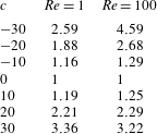
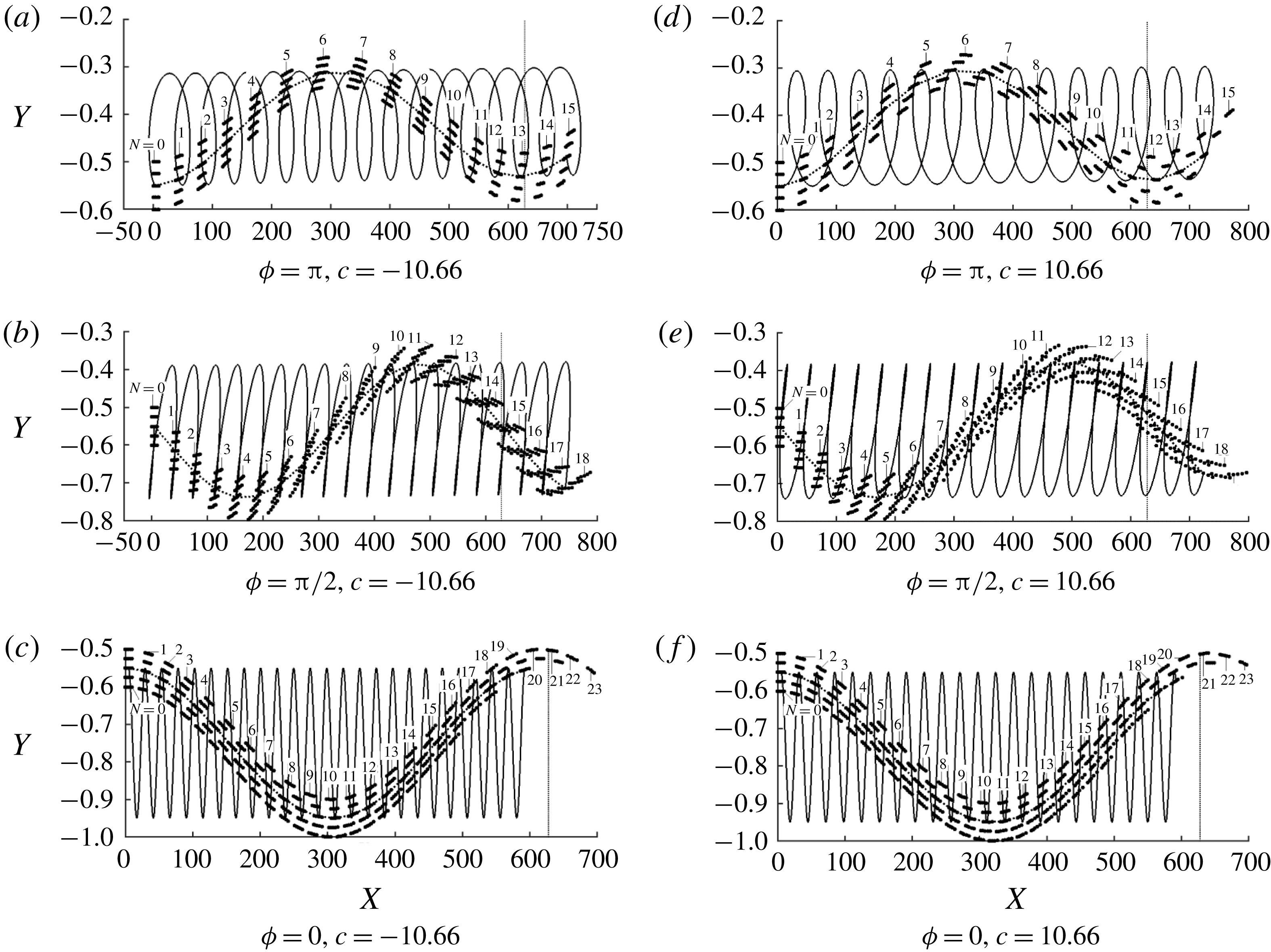
1 Introduction
Vibrating boundaries can be found in many engineering applications as well as in biological systems, but properties of flows exposed to such effects are not completely understood. This work is focused on the determination of the fundamental characteristics of such systems from two points of view, i.e. reduction of pressure gradient losses and mixing intensification. We shall focus attention on the laminar flows where drag reduction and mixing are difficult to achieve.
The existing literature relevant to the first question is focused on the peristaltic effect, where the fluid is driven along a conduit by inducing proper wall deformations. There are numerous examples of this effect in human bodies, e.g. transport of urine from the kidney to the bladder, transport of food through the gullet, bile movement from the gall-bladder to the duodenum as well as ovum movement in the fallopian tube. The same effect is utilized in technical applications, e.g. roller pumps whose components do not come into a direct contact with the fluid. A review by Jaffrin & Shapiro (Reference Jaffrin and Shapiro1971) provides an excellent introduction to this topic. More recent contributions include the analysis of fluid transport in finite-length tubes (Meijing & Brasseur Reference Meijing and Brasseur1993), micro-pumping (Aboelkassem & Staples Reference Aboelkassem and Staples2012), the description of the effects of channel asymmetry (Ramachandra & Mishra Reference Ramachandra Rao and Mishra2004) and the determination of the role played by non-Newtonian effects (El-Shehawy, El-Dabe & El-Desoky Reference El-Shehawy, El-Dabe and I.M2006; Hayat, Ali & Asghar Reference Hayat, Ali and Asghar2007; Ali et al. Reference Ali, Sajid, Abbas and Javed2010). A relation between the external forces, the tube elasticity and the resulting pumping effectiveness has been determined (Takagi & Balmforth Reference Takagi and Balmforth2011a ) and used in the analysis of the pumping of rigid objects (Takagi & Balmforth Reference Takagi and Balmforth2011b ).
The peristaltic effect is a good candidate for the development of drag reducing strategies, although such applications have yet to be properly explored. This is an active flow control method requiring energy input with the proper selection of the amplitude, shape and phase speeds of the waves playing an important role. It is known that the reduction of the pressure gradient can be achieved using suction/blowing waves (Min et al. Reference Min, Kang, Speyer and Kim2006; Marusic, Joseph & Nahesh Reference Marusic, Joseph and Nahesh2007). As the cost of energy input required for the creation of such waves is higher than the energy savings associated with smaller pressure gradients (Bewley Reference Bewley2009; Fukagata, Sugiyama & Kasagi Reference Fukagata, Sugiyama and Kasagi2009), these waves should be viewed as a different propulsion method. Similar waves can lead to relaminarization of turbulent flows (Mamori, Iwamoto & Marata Reference Mamori, Iwamoto and Marata2014) which provides a different mechanism for reduction of pressure losses and reduction of the overall energy expenditure. Turbulent drag reduction can be achieved using the in-plane transverse wall oscillations (Quadrio Reference Quadrio2011; Agostini, Touber & Leschziner Reference Agostini, Touber and Leschziner2014). Analysis of flow changes induced by the deformation waves without the oversimplifying assumptions is more complex due to the variable conduit geometry. The recent direct numerical simulations (DNS) results demonstrate turbulent drag reduction through the wall-movement-induced reduction of the random component of Reynolds stresses as well as through the flow relaminarization (Nakanishi, Mamori & Fukagata Reference Nakanishi, Mamori and Fukagata2012). There are indications that spatio-temporal modulations created by such elastic waves are able to reduce pressure losses in laminar flows, however the available numerical results (Hœpffner and Fukagata Reference Hœpffner and Fukagata2009) are very limited. This analysis can be viewed as a continuation of the work of Hœpffner and Fukagata (Reference Hœpffner and Fukagata2009) with the goal of explaining how the wall motions lead to the formation of forces acting on the fluid and identification of the system parameters which lead to the reduction of pressure gradient. The question as to whether the reduction of pressure losses represents a drag reduction or an alternative propulsion method relying on surface vibrations will be addressed.
The second question, i.e. the question of mixing intensification, is directly related to the question of transport of scalar quantities across the channel which relies, in the case of laminar flows, on diffusion only. The creation of transverse fluid movement can intensify this process by several orders of magnitude (Bergles & Webb Reference Bergles and Webb1983). The first group of techniques relies on a purely mechanical mixing associated with the use of vortex generators and is very effective but carries a large pressure drag penalty (Fiebig Reference Fiebig1995a ,Reference Fiebig b , Reference Fiebig1998; Jacobi & Shah Reference Jacobi and Shah1995). The second group relies on the creation of secondary flows which provide the desired transverse movement. The use of transverse grooves for the creation of streamwise vortices through the centrifugal effects was studied in Gepner & Floryan (Reference Gepner and Floryan2016), Moradi, Budiman & Floryan (Reference Moradi, Budiman and Floryan2017) while the use of longitudinal grooves for creating highly unstable travelling waves was studied in Moradi & Floryan (Reference Moradi and Floryan2014), Mohammadi, Moradi & Floryan (Reference Mohammadi, Moradi and Floryan2015), Yadav, Gepner & (Reference Yadav, Gepner and Szumbarski2017). Analysis of competition between the new waves and the classical Tollmien–Schlichting (TS) waves and determination as to whether the new waves offer any advantages over the TS waves were discussed in Moradi et al. (Reference Moradi, Budiman and Floryan2017). The third group relies on the promotion of the laminar–turbulent transition under subcritical conditions (Fiebig & Chen Reference Fiebig, Chen, Kaka, Bergles, Mayinger and Ync1999) as turbulent mixing is very effective. It is related to the second group as secondary flows represent different stages of the transition process and provide means for its acceleration if this is what is desired. The fourth group relies on the use of flow modifications to create chaotic advection (Aref Reference Aref1984; Stroock et al. Reference Stroock, Dertinger, Ajdari, Mezič, Stone and Whitesides2002; Sturman, Ottino & Wiggins Reference Sturman, Ottino and Wiggins2006). The focus of the present analysis is on a fifth group of methods, i.e. methods which rely on mechanical mixing induced by wall vibrations. Selverov & Stone (Reference Selverov and Stone2001) considered the use of small amplitude and high frequency waves propagating in rectangular cavities for this purpose. Jiménez-Lozano, Sen & Dunn (Reference Jiménez-Lozano, Sen and Dunn2009) studied peristaltic-effect-induced particle transport with application to ureter. It is not certain if vibrations can produce chaotic advection. Another form of vibrations, i.e. pulsations in the form of standing waves, was used to increase mixing through the creation of a steady streaming (Carlsson, Sen & Löfdahl Reference Carlsson, Sen and Löfdahl2005). Vibrations may also induce bifurcations leading to secondary flows which would intensify mixing, as demonstrated in the case of stationary grooves by Gepner & Floryan (Reference Gepner and Floryan2016), Moradi et al. (Reference Moradi, Budiman and Floryan2017).
This work is focused on the modifications of channel flows resulting from the transverse vibrations of bounding walls in the form of travelling waves. Such vibrations can be viewed as a dynamically evolving roughness, as waves with zero phase speed reduce to stationary grooves (stationary roughness). Waves can be created using properly distributed piezoelectric pistons with the relevant phase differences. The reference case, i.e. stationary grooves, has been subject to extensive studies which have determined both the pressure losses (Mohammadi & Floryan Reference Mohammadi and Floryan2012, Reference Mohammadi and Floryan2013a ,Reference Mohammadi and Floryan b ) as well as the stability limits (Floryan Reference Floryan2003, Reference Floryan2015; Floryan & Floryan Reference Floryan and Floryan2009; Gepner & Floryan Reference Gepner and Floryan2016). We shall focus this work on the potential use of such vibrations for the reduction of pressure losses and mixing intensification and shall relegate the analysis of the stability question to the following work. Accordingly, we focus on the direct system response, i.e. a forced response to the actuation which produces spatio-temporal flow modulation. Transverse vibrations produce an effect similar to that achieved with mechanical pistons and thus can create both a peristaltic effect as well as direct mechanical mixing without the need for initiation of secondary effects. We shall intentionally keep the Reynolds number small to avoid creation of secondary flows. It is known that small-amplitude surface waves may destabilize the Tollmien–Schlichting waves through a resonance (Floryan, Szumbarski & Wu Reference Floryan, Szumbarski and Wu2002). It is also expected that the finite-amplitude waves may initiate other processes similar to those found in the case of stationary grooves referred to above. In our model problem, the surface waves propagate along a channel where a laminar flow is driven by a constant pressure gradient. Their effect is assessed by determining the additional pressure gradient required to maintain the same flow rate in the vibrating as in the stationary channels. Variations and distributions of surface forces acting on the fluid are investigated and the mechanics of drag generation are illuminated. Particle trajectories are analysed, especially their transverse component as it directly contributes to mixing. This work provides a thorough explanation of different flow responses and the critical wave speeds separating them and makes a connection between the characteristics of vibrations and the pressure losses and the pattern of particle trajectories.
We need to note that there is a related class of problems, i.e. flows in conduits with pulsating walls with well-defined temporal characteristics but spatially constant amplitudes, which exhibits a very intriguing physics (Secomb Reference Secomb1978; Hall & Papageorgiou Reference Hall and Papageorgiou1999; Espin & Papageorgiou Reference Espin and Papageorgiou2012). Such pulsations may lead either to an increase in or a reduction of the flow rate depending on the Womersley number (Mingalev, Lyubimova & Filippov Reference Mingalev, Lyubimova and Filippov2015) but the physics underlying these effects is completely different from the processes analysed in the present work.
This presentation is organized as follows. Section 2 provides the problem formulation. Section 3 describes the solution method. Section 4 discusses the flow field modifications associated with single-wall vibrations. Section 5 presents an analysis of the forces acting on the fluid and identifies conditions leading to the reduction of pressure losses. Section 6 discusses changes in the system response associated with changes of the flow Reynolds number. Section 7 is focused on vibration-induced mixing augmentation. Section 8 discusses effects of two-wall vibrations and the phase shift between them. Section 9 provides a short summary of the main conclusions. The reader may note that the same principles apply to pipes with vibrating walls but details of the flow response can be different and, obviously, conclusions reached in the case of the two-wall vibrations do not apply.
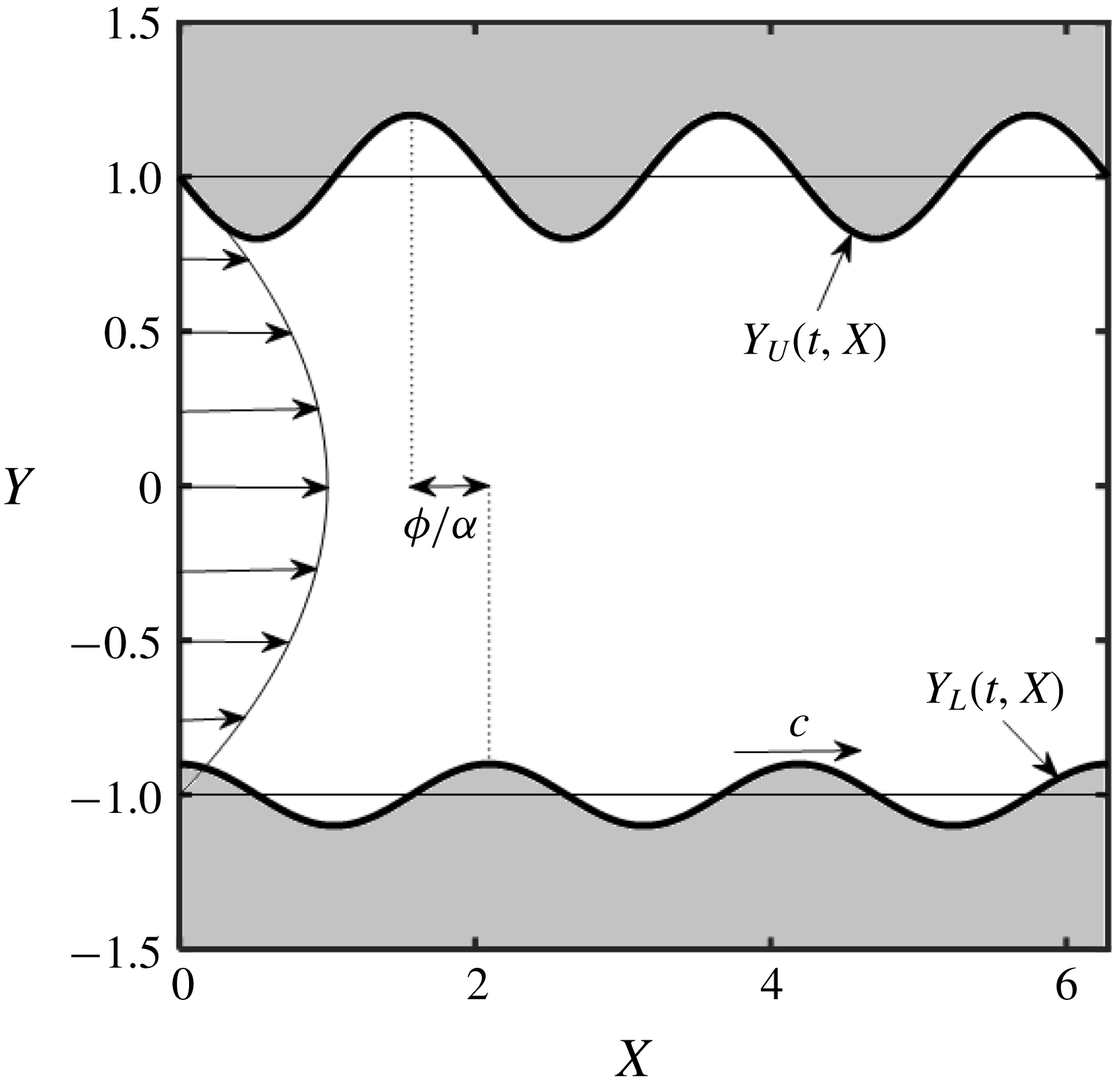
Channel with vibrating walls.

2 Problem formulation
Consider steady, two-dimensional flow of a fluid confined in a channel bounded by two parallel walls extending to
 $\pm \infty$
in the
 $X$
-direction and placed at a distance
 $2h$
apart, as shown in figure 1. The flow is driven in the positive
 $X$
-direction by a pressure gradient resulting in the velocity, pressure, streamfunction and flow rate of the form
 $$\begin{eqnarray}\displaystyle \boldsymbol{v}_{0}(X,Y)=[1-Y^{2},0],\quad p_{0}(X,Y)=-2X/Re,\quad Q_{0}={\textstyle \frac{4}{3}}, & & \displaystyle\end{eqnarray}$$
where
 $\boldsymbol{v}_{0}=[u_{0},v_{0}]$
denotes the velocity vector scaled with the maximum of the
 $X$
-velocity
 $u_{max}$
,
 $p_{0}$
stands for the pressure scaled with
 $\unicode[STIX]{x1D70C}u_{max}^{2}$
where
 $\unicode[STIX]{x1D70C}$
stands for the density,
 $Q_{0}$
denotes the flow rate, the Reynolds number is defined as
 $Re=u_{max}h/\unicode[STIX]{x1D708}$
where
 $\unicode[STIX]{x1D708}$
stands for the kinematic viscosity and
 $h$
has been used as the length scale. The flow is modified by imposing wall vibrations in the form of travelling waves with known amplitudes. The resulting channel geometry is described as
 $$\begin{eqnarray}\displaystyle Y_{U}(t,X)=1+A_{U}\cos [\unicode[STIX]{x1D6FC}(X-ct)+\unicode[STIX]{x1D719}],\quad Y_{L}(t,X)=-1+A_{L}\cos [\unicode[STIX]{x1D6FC}(X-ct)],\qquad & & \displaystyle\end{eqnarray}$$
where the subscripts
 $L$
and
 $U$
refer to the lower and upper walls, respectively,
 $A_{U}$
and
 $A_{L}$
are the wave amplitudes,
 $\unicode[STIX]{x1D706}=2\unicode[STIX]{x03C0}/\unicode[STIX]{x1D6FC},\unicode[STIX]{x1D6FC}$
and
 $c$
stand for the wavelength, wavenumber and phase speed and
 $\unicode[STIX]{x1D719}$
denotes the phase difference between the upper and lower waves. The resulting two-dimensional flow is described by the unsteady Navier–Stokes and continuity equations subject to boundary conditions of the form
 $$\begin{eqnarray}\displaystyle & \displaystyle u[t,X,Y_{U}(t,X)]=0,\quad v[t,X,Y_{U}(t,X)]=\frac{\unicode[STIX]{x2202}Y_{U}(t,X)}{\unicode[STIX]{x2202}t}=A_{U}\unicode[STIX]{x1D6FC}c\sin [\unicode[STIX]{x1D6FC}(X-ct)+\unicode[STIX]{x1D719}],\qquad & \displaystyle\end{eqnarray}$$
 $$\begin{eqnarray}\displaystyle & \displaystyle u[t,X,Y_{L}(t,X)]=0,\quad v[t,X,Y_{L}(t,X)]=\frac{\unicode[STIX]{x2202}Y_{L}(t,X)}{\unicode[STIX]{x2202}t}=A_{L}\unicode[STIX]{x1D6FC}c\sin [\unicode[STIX]{x1D6FC}(X-ct)], & \displaystyle\end{eqnarray}$$
 $(u,v)$
denote the (
 $X,Y$
)-components of the velocity vector and
 $h/u_{max}$
is the time scale. The determination as to whether the surface vibrations can lead to a reduction of pressure losses is carried out by evaluating pressure gradients required to carry the same flow rate through the stationary and vibrating channels. This leads to the imposition of the flow rate constraint of the form
 $$\begin{eqnarray}\displaystyle Q(t,X)|_{mean}=\left[\int _{Y_{L}(t,X)}^{Y_{U}(t,X)}u(t,X,Y)\,\text{d}Y\right]_{mean}={\textstyle \frac{4}{3}}. & & \displaystyle\end{eqnarray}$$
The resulting pressure gradient is represented as
 $$\begin{eqnarray}\displaystyle -\!\left.\frac{\unicode[STIX]{x2202}p}{\unicode[STIX]{x2202}X}\right|_{mean}=\frac{2}{Re}-B, & & \displaystyle\end{eqnarray}$$
where
 $p$
denotes pressure and
 $B$
is the unknown pressure gradient correction resulting from vibrations. Positive
 $B$
values correspond to a reduction of the pressure gradient below that associated with the flow in a stationary channel.
The fluid movement is resisted by forces acting on the fluid at the walls. The stress
 $\boldsymbol{f}=[f_{X},f_{Y}]$
acting at the lower wall can be expressed as
 $$\begin{eqnarray}\displaystyle Ref_{X}=Ref_{X,visc}+Ref_{X,pres}=\left[2n_{L,X}\frac{\unicode[STIX]{x2202}u}{\unicode[STIX]{x2202}X}+n_{L,Y}\left(\frac{\unicode[STIX]{x2202}u}{\unicode[STIX]{x2202}Y}+\frac{\unicode[STIX]{x2202}v}{\unicode[STIX]{x2202}X}\right)\right]_{Y_{L}(t,X)}-[Ren_{L,X}p]_{Y_{L}(t,X)}, & & \displaystyle \nonumber\\ \displaystyle & & \displaystyle\end{eqnarray}$$
 $$\begin{eqnarray}\displaystyle Ref_{Y}=Ref_{Y,visc}+Ref_{Y,pres}=\left[n_{L,X}\left(\frac{\unicode[STIX]{x2202}u}{\unicode[STIX]{x2202}Y}+\frac{\unicode[STIX]{x2202}v}{\unicode[STIX]{x2202}X}\right)+2n_{L,Y}\frac{\unicode[STIX]{x2202}v}{\unicode[STIX]{x2202}Y}\right]_{Y_{L}(t,X)}-[Ren_{L,Y}p]_{Y_{L}(t,X)}, & & \displaystyle \nonumber\\ \displaystyle & & \displaystyle\end{eqnarray}$$
 $visc$
and
 $pres$
identify friction and pressure contributions, respectively, and the outward normal unit vector has the form
 $$\begin{eqnarray}\displaystyle \boldsymbol{n}_{L}=[n_{L,X},n_{L,Y}]=[-A_{L}\unicode[STIX]{x1D6FC}\sin \{\unicode[STIX]{x1D6FC}(X-ct)\},-1]/N_{L} & & \displaystyle\end{eqnarray}$$
with
 $N_{L}=[1+(A_{L}\unicode[STIX]{x1D6FC}\sin [\unicode[STIX]{x1D6FC}(X-ct)])^{2}]^{1/2}$
. The total force acting at the lower wall per unit channel length
 $\boldsymbol{F}=[F_{X},F_{Y}]=[(F_{X,visc}+F_{X,pres}),(F_{Y,visc}+F_{Y,pres})]$
is determined through proper integration, i.e.
 $$\begin{eqnarray}\displaystyle Re[F_{X,visc},F_{X,pres},F_{Y,visc},F_{Y,pres}]=Re\unicode[STIX]{x1D706}^{-1}\int _{\unicode[STIX]{x1D6FE}}^{\unicode[STIX]{x1D6FE}+2\unicode[STIX]{x03C0}/\unicode[STIX]{x1D6FC}}[f_{X,visc},f_{X,pres},f_{Y,visc},f_{Y,pres}]N_{L}\,\text{d}X. & & \displaystyle \nonumber\\ \displaystyle & & \displaystyle\end{eqnarray}$$
The stresses
 $\boldsymbol{g}=[g_{X},g_{Y}]=[(g_{X,visc}+g_{X,pres}),(g_{Y,visc}+g_{Y,pres})]$
and the total force
 $\boldsymbol{G}=[G_{X},G_{Y}]=[(G_{X,visc}+G_{X,pres}),(G_{Y,visc}+G_{Y,pres})]$
acting at the upper wall can be determined in a similar manner. The total force
 $\boldsymbol{H}_{tot}$
acting on the fluid at both walls is defined as
 $$\begin{eqnarray}\displaystyle \boldsymbol{H}_{tot}=[H_{tot,X},H_{tot,Y}]=[(F_{X}+G_{X}),(F_{Y}+G_{Y})] & & \displaystyle\end{eqnarray}$$
and must be balanced by the pressure gradient multiplied by the channel cross-sectional area.
The energy cost of the actuation is one of the quantities of interest and, especially, whether this energy is higher or lower than the energy savings associated with reduction of pressure losses. Theoretical predictions suggest that the actuation cost will be higher but these predictions are based on a smooth channel and actuation in the form of transpiration waves (Bewley Reference Bewley2009; Fukagata et al. Reference Fukagata, Sugiyama and Kasagi2009).
Changes of pumping power
 $\unicode[STIX]{x0394}{\wp}$
associated with vibrations can be evaluated as
 $$\begin{eqnarray}\displaystyle \unicode[STIX]{x0394}{\wp}={\wp}_{0}-{\wp}_{vib}=\frac{8}{3Re}-\frac{4}{3}\left(\frac{2}{Re}-B\right)=\frac{4}{3}B, & & \displaystyle\end{eqnarray}$$
where
 ${\wp}_{0}$
denotes pumping power per unit length and width of an unmodified channel and
 ${\wp}_{vib}$
stands for the same power in a vibrating channel. The actuation power at the lower wall can be computed as
 $$\begin{eqnarray}\displaystyle {\wp}_{act}=\frac{1}{\unicode[STIX]{x1D706}}\int _{0}^{\unicode[STIX]{x1D706}}N_{L}(vf_{Y})|_{y_{L}(t,X)}\,\text{d}X. & & \displaystyle\end{eqnarray}$$
A similar expression can be developed for the actuation power at the upper wall. Comparison of both gives the net energy savings defined as
 $$\begin{eqnarray}\displaystyle Re\unicode[STIX]{x0394}{\wp}_{net}=Re(\unicode[STIX]{x0394}{\wp}-{\wp}_{act}). & & \displaystyle\end{eqnarray}$$
Positive values of
 $Re\unicode[STIX]{x0394}{\wp}_{net}$
identify waves which induce pressure losses reduction large enough to overcome energy cost associated with the actuation.
3 Solution method
We shall focus attention on vibrations in the form of long waves propagating along the lower wall, i.e.
 $A_{L}=A$
,
 $A_{U}=0$
. Use of the Galileo transformation, i.e.
 $y=Y$
,
 $x=X-ct$
, results in a stationary problem of the form
 $$\begin{eqnarray}\displaystyle \left.\begin{array}{@{}c@{}}\displaystyle (u-c)\frac{\unicode[STIX]{x2202}u}{\unicode[STIX]{x2202}x}+v\frac{\unicode[STIX]{x2202}u}{\unicode[STIX]{x2202}y}=-\frac{\unicode[STIX]{x2202}p}{\unicode[STIX]{x2202}x}+Re^{-1}\left(\frac{\unicode[STIX]{x2202}^{2}u}{\unicode[STIX]{x2202}x^{2}}+\frac{\unicode[STIX]{x2202}^{2}u}{\unicode[STIX]{x2202}y^{2}}\right)\!,\\ \displaystyle (u-c)\frac{\unicode[STIX]{x2202}v}{\unicode[STIX]{x2202}x}+v\frac{\unicode[STIX]{x2202}v}{\unicode[STIX]{x2202}y}=-\frac{\unicode[STIX]{x2202}p}{\unicode[STIX]{x2202}y}+Re^{-1}\left(\frac{\unicode[STIX]{x2202}^{2}v}{\unicode[STIX]{x2202}x^{2}}+\frac{\unicode[STIX]{x2202}^{2}v}{\unicode[STIX]{x2202}y^{2}}\right)\!,\end{array}\!\right\} & & \displaystyle\end{eqnarray}$$
 $$\begin{eqnarray}\displaystyle \frac{\unicode[STIX]{x2202}u}{\unicode[STIX]{x2202}x}+\frac{\unicode[STIX]{x2202}v}{\unicode[STIX]{x2202}y}=0, & & \displaystyle\end{eqnarray}$$
 $$\begin{eqnarray}\displaystyle y=1:\quad u=0,v=0;\quad y=y_{L}(x)=-1+A\cos (\unicode[STIX]{x1D6FC}x):\quad u=0,v=A\unicode[STIX]{x1D6FC}c\sin (\unicode[STIX]{x1D6FC}x), & & \displaystyle \nonumber\\ \displaystyle & & \displaystyle\end{eqnarray}$$
 $$\begin{eqnarray}\displaystyle Q(x)|_{mean}=\left.\left(\int _{y_{L}(x)}^{1}u(x,y)\,\text{d}y\right)\right|_{mean}={\textstyle \frac{4}{3}}. & & \displaystyle\end{eqnarray}$$
The solution domain is regularized using the transformation
 $$\begin{eqnarray}\displaystyle \unicode[STIX]{x1D709}=\unicode[STIX]{x1D6FC}x,\quad \unicode[STIX]{x1D702}=(y-1)\left[1-{\textstyle \frac{1}{2}}A\cos (\unicode[STIX]{x1D6FC}x)\right]^{-1}+1, & & \displaystyle\end{eqnarray}$$
which maps the original irregular domain into
 $\unicode[STIX]{x1D702}\in \langle -1,1\rangle$
and introduces a wavelength-based scale in the
 $x$
-direction to capture the wave-induced flow modulations. Field equations, boundary conditions and constraint after transformation can be written as
 $$\begin{eqnarray}\displaystyle & & \displaystyle \frac{\unicode[STIX]{x2202}^{2}u}{\unicode[STIX]{x2202}\unicode[STIX]{x1D702}^{2}}+[F_{1}-F_{2}(u-c)-F_{3}v]\frac{\unicode[STIX]{x2202}u}{\unicode[STIX]{x2202}\unicode[STIX]{x1D702}}+F_{4}\frac{\unicode[STIX]{x2202}^{2}u}{\unicode[STIX]{x2202}\unicode[STIX]{x1D709}\unicode[STIX]{x2202}\unicode[STIX]{x1D702}}+F_{5}\frac{\unicode[STIX]{x2202}^{2}u}{\unicode[STIX]{x2202}\unicode[STIX]{x1D709}^{2}}\nonumber\\ \displaystyle & & \displaystyle -\,F_{6}(u-c)\frac{\unicode[STIX]{x2202}u}{\unicode[STIX]{x2202}\unicode[STIX]{x1D709}}-F_{6}\frac{\unicode[STIX]{x2202}p}{\unicode[STIX]{x2202}\unicode[STIX]{x1D709}}-F_{2}\frac{\unicode[STIX]{x2202}p}{\unicode[STIX]{x2202}\unicode[STIX]{x1D702}}=0,\end{eqnarray}$$
 $$\begin{eqnarray}\displaystyle & \displaystyle \frac{\unicode[STIX]{x2202}^{2}v}{\unicode[STIX]{x2202}\unicode[STIX]{x1D702}^{2}}+[F_{1}-F_{2}(u-c)-F_{3}v]\frac{\unicode[STIX]{x2202}v}{\unicode[STIX]{x2202}\unicode[STIX]{x1D702}}+F_{4}\frac{\unicode[STIX]{x2202}^{2}v}{\unicode[STIX]{x2202}\unicode[STIX]{x1D709}\unicode[STIX]{x2202}\unicode[STIX]{x1D702}}+F_{5}\frac{\unicode[STIX]{x2202}^{2}v}{\unicode[STIX]{x2202}\unicode[STIX]{x1D709}^{2}}-F_{6}(u-c)\frac{\unicode[STIX]{x2202}v}{\unicode[STIX]{x2202}\unicode[STIX]{x1D709}}-F_{3}\frac{\unicode[STIX]{x2202}p}{\unicode[STIX]{x2202}\unicode[STIX]{x1D702}}=0, & \displaystyle \nonumber\\ \displaystyle & & \displaystyle\end{eqnarray}$$
 $$\begin{eqnarray}\displaystyle & \displaystyle \unicode[STIX]{x1D6FC}\frac{\unicode[STIX]{x2202}u}{\unicode[STIX]{x2202}\unicode[STIX]{x1D709}}+F_{7}\frac{\unicode[STIX]{x2202}u}{\unicode[STIX]{x2202}\unicode[STIX]{x1D702}}+F_{8}\frac{\unicode[STIX]{x2202}v}{\unicode[STIX]{x2202}\unicode[STIX]{x1D702}}=0, & \displaystyle\end{eqnarray}$$
 $$\begin{eqnarray}\displaystyle \left.\begin{array}{@{}c@{}}\displaystyle u(\unicode[STIX]{x1D709},1)=v(\unicode[STIX]{x1D709},1)=0,\quad u(\unicode[STIX]{x1D709},-1)=0,\\ \displaystyle v(\unicode[STIX]{x1D709},-1)=cA\unicode[STIX]{x1D6FC}\sin (\unicode[STIX]{x1D709}),\quad \left(G_{1}\int _{-1}^{1}u\,\text{d}\unicode[STIX]{x1D702}\right)_{mean}={\textstyle \frac{8}{3}}\end{array}\right\} & & \displaystyle\end{eqnarray}$$
with all coefficients defined in appendix A. The unknowns are represented as expansions of the form
 $$\begin{eqnarray}\displaystyle [u,v]=[\tilde{u} _{0},\tilde{v}_{0}]+\unicode[STIX]{x1D6FC}[\tilde{u} _{1},\tilde{v}_{1}]+O(\unicode[STIX]{x1D6FC}^{2}),\quad p=\unicode[STIX]{x1D6FC}^{-1}\tilde{p}_{-1}+\tilde{p}_{0}+O(\unicode[STIX]{x1D6FC}), & & \displaystyle\end{eqnarray}$$
the variable coefficients in (3.3) are replaced by their small-
 $\unicode[STIX]{x1D6FC}$
approximations (see appendix A), (3.5) is substituted into (3.3)–(3.4) and terms with the same order of magnitude are separated resulting in a sequence of problems with the leading-order system being of the form
 $$\begin{eqnarray}\displaystyle \frac{\unicode[STIX]{x2202}^{2}\tilde{u} _{0}}{\unicode[STIX]{x2202}\unicode[STIX]{x1D702}^{2}}-\frac{1}{2}ReG_{1}\tilde{v}_{0}\frac{\unicode[STIX]{x2202}\tilde{u} _{0}}{\unicode[STIX]{x2202}\unicode[STIX]{x1D702}}-\frac{1}{4}ReG_{1}^{2}\frac{\unicode[STIX]{x2202}\tilde{p}_{-1}}{\unicode[STIX]{x2202}\unicode[STIX]{x1D709}}+\frac{1}{4}ReA\sin (\unicode[STIX]{x1D709})G_{1}(\unicode[STIX]{x1D702}-1)\frac{\unicode[STIX]{x2202}\tilde{p}_{-1}}{\unicode[STIX]{x2202}\unicode[STIX]{x1D702}}=0, & & \displaystyle\end{eqnarray}$$
 $$\begin{eqnarray}\displaystyle \frac{\unicode[STIX]{x2202}\tilde{p}_{-1}}{\unicode[STIX]{x2202}\unicode[STIX]{x1D702}}=0,\quad \frac{\unicode[STIX]{x2202}\tilde{v}_{0}}{\unicode[STIX]{x2202}\unicode[STIX]{x1D702}}=0,\quad \tilde{u} _{0}(\unicode[STIX]{x1D709},\pm 1)=\tilde{v}_{0}(\unicode[STIX]{x1D709},\pm 1)=0,\quad \left(G_{1}\int _{\unicode[STIX]{x1D702}=-1}^{\unicode[STIX]{x1D702}=1}\tilde{u} _{0}\,\text{d}\unicode[STIX]{x1D702}\right)_{mean}=\frac{8}{3}. & & \displaystyle \nonumber\\ \displaystyle & & \displaystyle\end{eqnarray}$$
Its solution can be easily determined, i.e.
 $$\begin{eqnarray}\displaystyle \frac{\text{d}\tilde{p}_{-1}}{\text{d}\unicode[STIX]{x1D709}}=-16Re^{-1}G_{1}^{-3}+c12ARe^{-1}G_{1}^{-3}\cos (\unicode[STIX]{x1D709}), & & \displaystyle\end{eqnarray}$$
 $$\begin{eqnarray}\displaystyle \tilde{u} _{0}=2(1-\unicode[STIX]{x1D702}^{2})G_{1}^{-1}-c{\textstyle \frac{3}{2}}A(1-\unicode[STIX]{x1D702}^{2})\cos (\unicode[STIX]{x1D709})G_{1}^{-1},\quad \tilde{v}_{0}=0. & & \displaystyle\end{eqnarray}$$
Integration of (3.7a ) results in an explicit expression for pressure in the form
 $$\begin{eqnarray}\displaystyle & & \displaystyle Re\tilde{p}_{-1}=-\left(4+\frac{A^{2}}{2}\right)K(\unicode[STIX]{x1D709})-A\sin (\unicode[STIX]{x1D709})\left(1-\frac{A^{2}}{4}\right)^{-2}G_{1}^{-2}\left[8-\frac{A^{2}}{2}-3A\cos (\unicode[STIX]{x1D709})\right]\nonumber\\ \displaystyle & & \displaystyle \quad -\,\frac{c}{4}\left\{-9A^{2}K(\unicode[STIX]{x1D709})+A\sin (\unicode[STIX]{x1D709})\left(1-\frac{A^{2}}{4}\right)^{-2}G_{1}^{-2}[-3A^{2}-24+A(6+3A^{2})\cos (\unicode[STIX]{x1D709})]\right\},\nonumber\\ \displaystyle & & \displaystyle\end{eqnarray}$$
where
 $$\begin{eqnarray}\displaystyle K(\unicode[STIX]{x1D709})=\left(\!1-\frac{A^{2}}{4}\right)^{-5/2}\!\left\{\text{arctan}\!\left[\left(1+\frac{A}{2}\right)^{1/2}\left(1-\frac{A}{2}\right)^{-1/2}\tan \left(\frac{\unicode[STIX]{x1D709}}{2}\right)\right]+\unicode[STIX]{x03C0}\left\lfloor \frac{\unicode[STIX]{x1D709}+\unicode[STIX]{x03C0}}{2\unicode[STIX]{x03C0}}\right\rfloor \!\right\}. & & \displaystyle \nonumber\\ \displaystyle & & \displaystyle\end{eqnarray}$$
In the above, symbol
 $\lfloor \ldots \rfloor$
stands for the floor function, which has been added to remove spurious discontinuities associated with the arctan function (Jeffrey & Rich Reference Jeffrey and Rich1994) and pressure is normalized with condition
 $\tilde{p}_{-1}(0)=0$
. Since
 $\text{d}\tilde{p}_{-1}/\text{d}\unicode[STIX]{x1D709}$
in (3.7a
) is an even function of
 $\unicode[STIX]{x1D709}$
, it can be expressed as a cosine Fourier expansion and integrated with respect to
 $\unicode[STIX]{x1D709}$
term by term to arrive at
 $$\begin{eqnarray}\displaystyle Re\tilde{p}_{-1} & = & \displaystyle \left(1-\frac{A^{2}}{4}\right)^{-5/2}\left[-2\left(1+\frac{A^{2}}{8}\right)+\frac{9}{8}cA^{2}\right]\unicode[STIX]{x1D709}\nonumber\\ \displaystyle & & \displaystyle +\,A\left(1-\frac{A^{2}}{4}\right)^{-5/2}\left[-3+\frac{3}{2}c\left(1+\frac{A^{2}}{2}\right)\right]\sin (\unicode[STIX]{x1D709})+\cdots \,,\end{eqnarray}$$
where the aperiodic term captures the mean pressure gradient.
The next-order system has the form
 $$\begin{eqnarray}\displaystyle & & \displaystyle \frac{\unicode[STIX]{x2202}^{2}\tilde{u} _{1}}{\unicode[STIX]{x2202}\unicode[STIX]{x1D702}^{2}}-\frac{1}{2}ReG_{1}\frac{\unicode[STIX]{x2202}\tilde{u} _{0}}{\unicode[STIX]{x2202}\unicode[STIX]{x1D702}}\tilde{v}_{1}-\frac{1}{4}ReG_{1}^{2}\frac{\unicode[STIX]{x2202}\tilde{p}_{0}}{\unicode[STIX]{x2202}\unicode[STIX]{x1D709}}+\frac{1}{4}ReA\sin (\unicode[STIX]{x1D709})G_{1}(\unicode[STIX]{x1D702}-1)\frac{\unicode[STIX]{x2202}\tilde{p}_{0}}{\unicode[STIX]{x2202}\unicode[STIX]{x1D702}}\nonumber\\ \displaystyle & & \displaystyle \quad =-\frac{1}{4}ReA\sin (\unicode[STIX]{x1D709})G_{1}(\unicode[STIX]{x1D702}-1)(\tilde{u} _{0}-c)\frac{\unicode[STIX]{x2202}\tilde{u} _{0}}{\unicode[STIX]{x2202}\unicode[STIX]{x1D702}}+\frac{1}{4}ReG_{1}^{2}(\tilde{u} _{0}-c)\frac{\unicode[STIX]{x2202}\tilde{u} _{0}}{\unicode[STIX]{x2202}\unicode[STIX]{x1D709}}\end{eqnarray}$$
 $$\begin{eqnarray}\displaystyle \frac{\unicode[STIX]{x2202}\tilde{p}_{0}}{\unicode[STIX]{x2202}\unicode[STIX]{x1D702}}=0,\quad \frac{\unicode[STIX]{x2202}\tilde{v}_{1}}{\unicode[STIX]{x2202}\unicode[STIX]{x1D702}}=\frac{1}{2}A(\unicode[STIX]{x1D702}-1)\sin (\unicode[STIX]{x1D709})\frac{\unicode[STIX]{x2202}\tilde{u} _{0}}{\unicode[STIX]{x2202}\unicode[STIX]{x1D702}}-\frac{1}{2}G_{1}\frac{\unicode[STIX]{x2202}\tilde{u} _{0}}{\unicode[STIX]{x2202}\unicode[STIX]{x1D709}}, & & \displaystyle\end{eqnarray}$$
 $$\begin{eqnarray}\displaystyle \left.\begin{array}{@{}c@{}}\displaystyle \tilde{u} _{1}(\unicode[STIX]{x1D709},1)=\tilde{v}_{1}(\unicode[STIX]{x1D709},1)=0,\quad \tilde{u} _{1}(\unicode[STIX]{x1D709},-1)=0,\\ \displaystyle \tilde{v}_{1}(\unicode[STIX]{x1D709},-1)=cA\sin (\unicode[STIX]{x1D709}),\quad \left(\int _{\unicode[STIX]{x1D702}=-1}^{\unicode[STIX]{x1D702}=1}\tilde{u} _{1}\,\text{d}\unicode[STIX]{x1D702}\right)_{mean}=0\end{array}\right\} & & \displaystyle\end{eqnarray}$$
and its solution can be written as
 $$\begin{eqnarray}\displaystyle & & \displaystyle \!\!\!\!\!\!\frac{\text{d}\tilde{p}_{0}}{\text{d}\unicode[STIX]{x1D709}}=\frac{96}{35}A\sin (\unicode[STIX]{x1D709})G_{1}^{-3}-\frac{c}{35}G_{1}^{-2}[18A^{2}G_{1}^{-1}\sin (2\unicode[STIX]{x1D709})+A(28+216G_{1}^{-1})\sin (\unicode[STIX]{x1D709})]\nonumber\\ \displaystyle & & \displaystyle \qquad +\,\frac{c^{2}}{70}G_{1}^{-2}[-27A^{3}G_{1}^{-1}\sin (3\unicode[STIX]{x1D709})+A^{2}(162G_{1}^{-1}-21)\sin (2\unicode[STIX]{x1D709})+168A\sin (\unicode[STIX]{x1D709})],\qquad \quad\end{eqnarray}$$
 $$\begin{eqnarray}\displaystyle \frac{\tilde{u} _{1}}{Re} & = & \displaystyle A\sin (\unicode[STIX]{x1D709})G_{1}^{-1}H_{8}+c\left[\frac{1}{2}G_{1}^{-1}A^{2}\sin (2\unicode[STIX]{x1D709})H_{5}+A(G_{1}^{-1}H_{6}+H_{7})\sin (\unicode[STIX]{x1D709})\right]\nonumber\\ \displaystyle & & \displaystyle +\,\frac{c^{2}}{2}\left[G_{1}^{-1}A^{3}H_{1}\sin (3\unicode[STIX]{x1D709})+A^{2}\left(G_{1}^{-1}H_{2}+\frac{3}{4}H_{3}\right)\sin (2\unicode[STIX]{x1D709})-\frac{3}{2}AH_{4}\sin (\unicode[STIX]{x1D709})\right],\qquad \quad\end{eqnarray}$$
 $$\begin{eqnarray}\displaystyle \tilde{v}_{1}=-2AG_{1}^{-1}H_{11}\sin (\unicode[STIX]{x1D709})-c2G_{1}^{-1}\left[-\frac{A^{2}}{2}\sin (2\unicode[STIX]{x1D709})H_{10}+AH_{9}\sin (\unicode[STIX]{x1D709})\right], & & \displaystyle\end{eqnarray}$$
 $$\begin{eqnarray}\displaystyle \tilde{p}_{0} & = & \displaystyle -\frac{48}{35}G_{1}^{-2}+\frac{12}{35}\left(1-\frac{A}{2}\right)^{-2}\nonumber\\ \displaystyle & & \displaystyle -\,\frac{c}{35}\left[-128G_{1}^{-2}+2(A+16)\left(1-\frac{A}{2}\right)^{-2}-8AG_{1}^{-2}\cos (\unicode[STIX]{x1D709})\right]\nonumber\\ \displaystyle & & \displaystyle +\,\frac{c^{2}}{35}\left[-84G_{1}^{-2}+3(7+A)\left(1-\frac{A}{2}\right)^{-2}-6\ln \frac{G_{1}}{2-A}+12AG_{1}^{-2}\cos (\unicode[STIX]{x1D709})\right]\nonumber\\ \displaystyle & & \displaystyle\end{eqnarray}$$
 $\tilde{p}_{0}$
being normalized with condition
 $\tilde{p}_{0}(0)=0$
.
4 Flow field modifications created by the one-wall vibrations
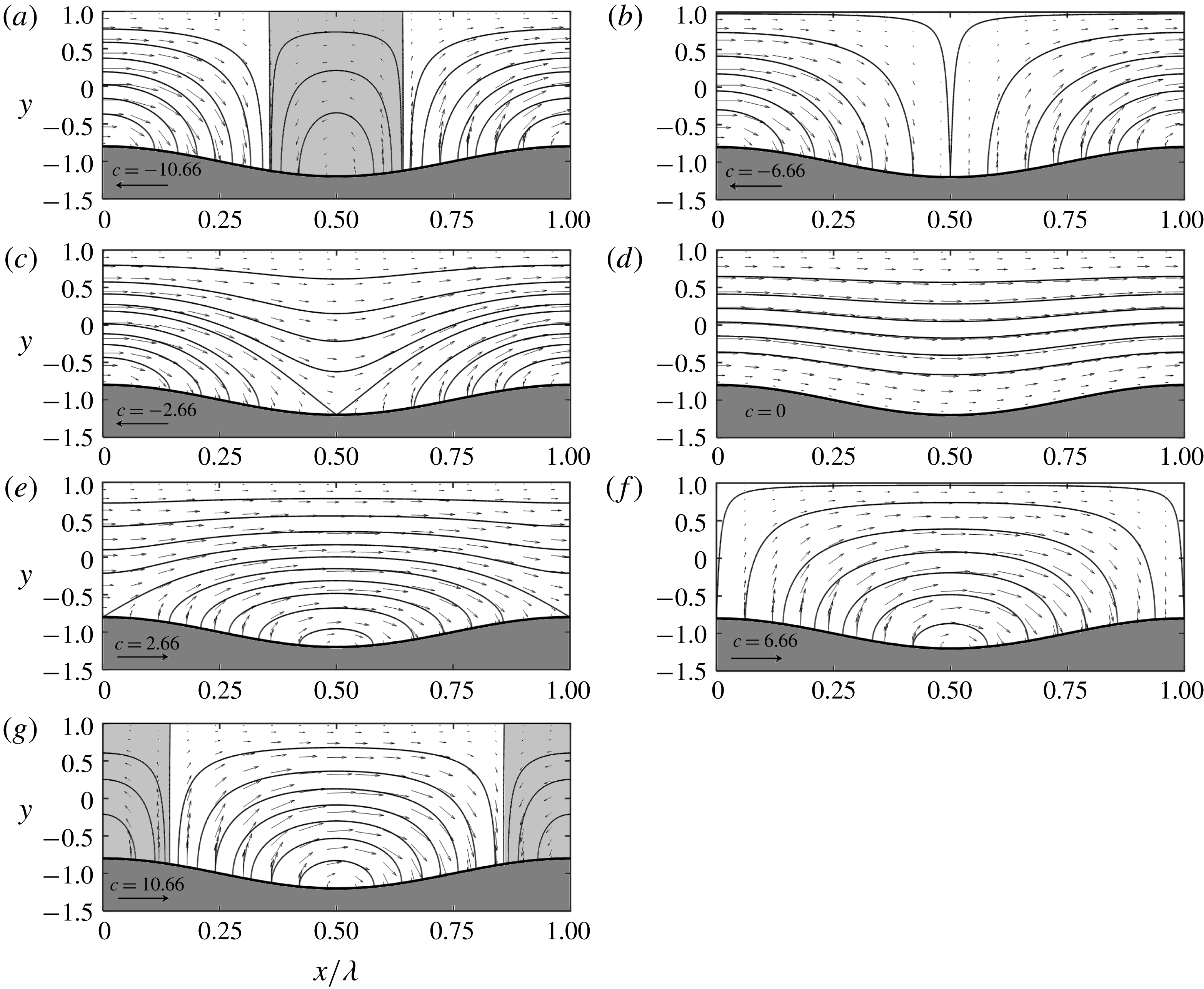
We begin the discussion with the small
 $Re$
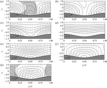
-flows. Modifications of the flow field are nearly symmetric with respect to the wave crest and strongly depend on the magnitude and direction of its phase speed, as illustrated in figure 2. The flow field created by stationary grooves (
 $c=0$
) shows gentle streamwise modulations (figure 2
d). Waves propagating in the streamwise direction result in more pronounced modulations with velocity increasing at the troughs and decreasing at the crests (see data for
 $c=2.66$
in figure 2
e). At
 $c=6.66$
, the fluid is brought to a complete stop at the cross-sections above the wave crests, thus dividing the flow field into separate pockets (figure 2
f). The wall shear stress and
 $\unicode[STIX]{x2202}u/\unicode[STIX]{x2202}y$
are reduced to zero at the crests, signalling the onset of flow separation. Further increase of
 $c$
leads to the formation of separation zones around the crests (see data for
 $c=10.66$
in figure 2
g). Change in the direction of wave propagation, i.e. waves now propagate upstream, creates qualitatively different spatial modulations with velocity increasing at the crests and decreasing at the troughs (figure 2
c). At
 $c=-6.66$
, the flow field separates into pockets centred around crests (figure 2
b). Fluid is brought to a complete stop at the cross-sections above troughs, and the wall shear stress and
 $\unicode[STIX]{x2202}u/\unicode[STIX]{x2202}y$
become zero at the troughs, suggesting an incipient flow separation. At
 $c=-10.66$
the flow field consists of separate zones of the forward moving fluid centred at the crests and the backward moving fluid centred at the troughs.
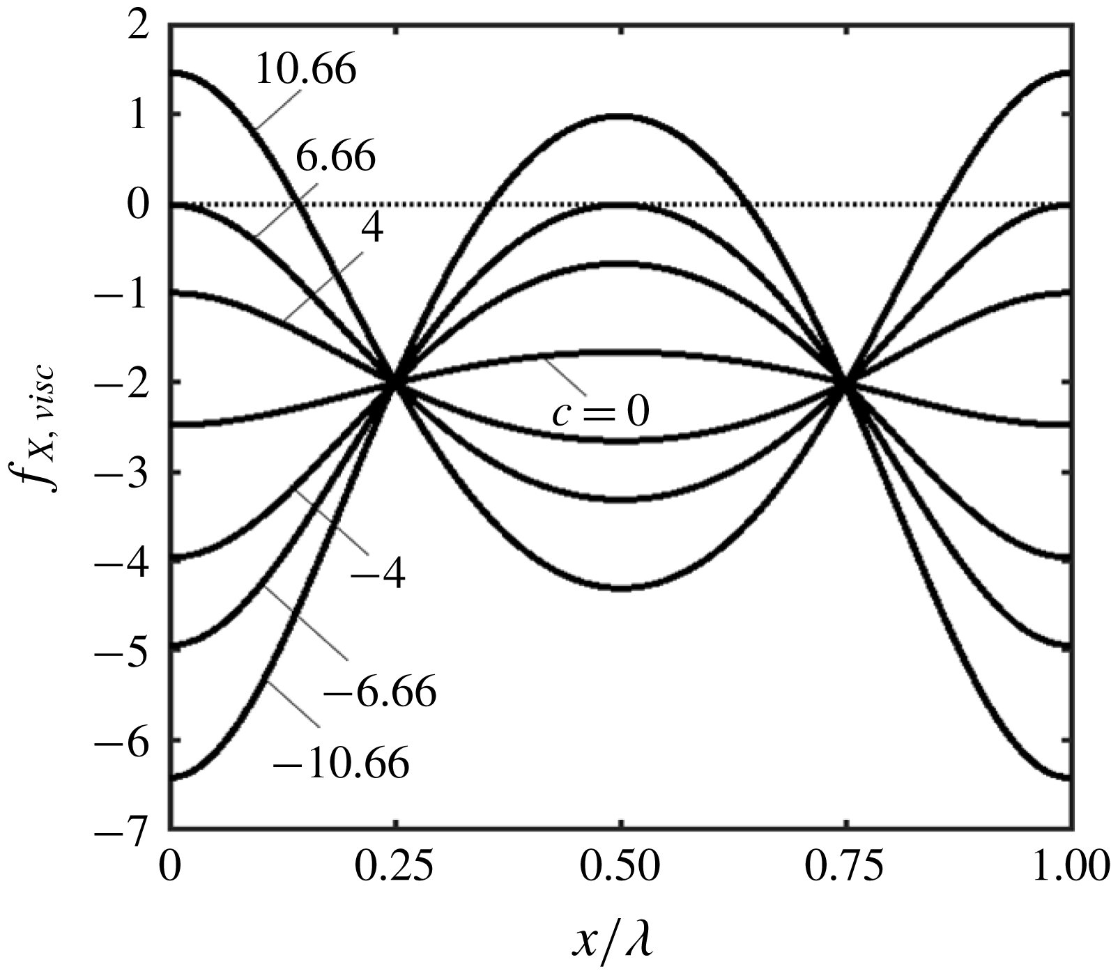
Details of the separation process can be deduced by looking at the wall shear
 $$\begin{eqnarray}\displaystyle Ref_{X,visc} & = & \displaystyle G_{1}^{-2}[-8+6cA\cos (\unicode[STIX]{x1D709})]\nonumber\\ \displaystyle & & \displaystyle +\,\unicode[STIX]{x1D6FC}ReG_{1}^{-1}\left\{\!{\textstyle \frac{32}{105}}A\sin (\unicode[STIX]{x1D709})G_{1}^{-1}\right.\nonumber\\ \displaystyle & & \displaystyle -\,c\left[{\textstyle \frac{62}{105}}A^{2}\sin (2\unicode[STIX]{x1D709})G_{1}^{-1}+A\left(-{\textstyle \frac{152}{105}}G_{1}^{-1}+{\textstyle \frac{16}{15}}\right)\sin (\unicode[STIX]{x1D709})\right]\nonumber\\ \displaystyle & & \displaystyle -\,c^{2}\left[-{\textstyle \frac{10}{7}}A^{3}\sin (3\unicode[STIX]{x1D709})G_{1}^{-1}+\left({\textstyle \frac{19}{35}}G_{1}^{-1}-{\textstyle \frac{7}{20}}\right)A^{2}\sin (2\unicode[STIX]{x1D709})\right.\nonumber\\ \displaystyle & & \displaystyle -\!\left.\left.{\textstyle \frac{1}{5}}A\sin (\unicode[STIX]{x1D709})\right]\!\right\}+O(\unicode[STIX]{x1D6FC}^{2}).\end{eqnarray}$$
The stress is negative everywhere for
 $-c_{sep}<c<c_{sep}$
, where
 $c_{sep}=(4/3)A^{-1}$
, and becomes zero at one point along the wall when
 $|c|=c_{sep}$
. As the flow is unsteady, these two wave speeds do not need to mark the onset of flow separation as they do not guarantee a change of the flow direction. Zeroing of the wall-normal derivative of the velocity vector does identify the change of direction and the relevant analysis shows that it occurs for the same conditions as the zeroing of the shear stress if the long wavelength waves are considered. Accordingly, we shall refer to
 $c_{sep}$
as the separation phase speed.
Plots of velocity fields for
 $Re=1$
,
 $A=0.2$
,
 $\unicode[STIX]{x1D6FC}=0.01$
and
 $c=-10.66,-6.66,-2.66,0,2.66,6.66,10.66$
in (a–g), respectively. Shaded areas identify zones with reverse flow direction.

When waves propagate in the streamwise direction, the stress is at first reduced to zero at the wave crest (
 $\unicode[STIX]{x1D709}=0,2\unicode[STIX]{x03C0}$
) and this happens when
 $c=c_{sep}$
. Further increase of
 $c$
results in the reversal of its direction and increase of the size of the zone with positive stress (see figure 3). When waves propagate in the upstream direction, the stress first becomes zero at the wave trough (
 $\unicode[STIX]{x1D709}=\unicode[STIX]{x03C0}$
) and this happens when
 $c=-c_{sep}$
. Further increase of
 $c$
results in the reversal of its direction and increase of the size of the zone with positive stress.
Distributions of
 $Ref_{X,visc}$
for
 $Re=1$
,
 $A=0.2$
,
 $\unicode[STIX]{x1D6FC}=0.01$
. The special value of
 $c$
for this case is
 $c_{sep}=6.66$
.

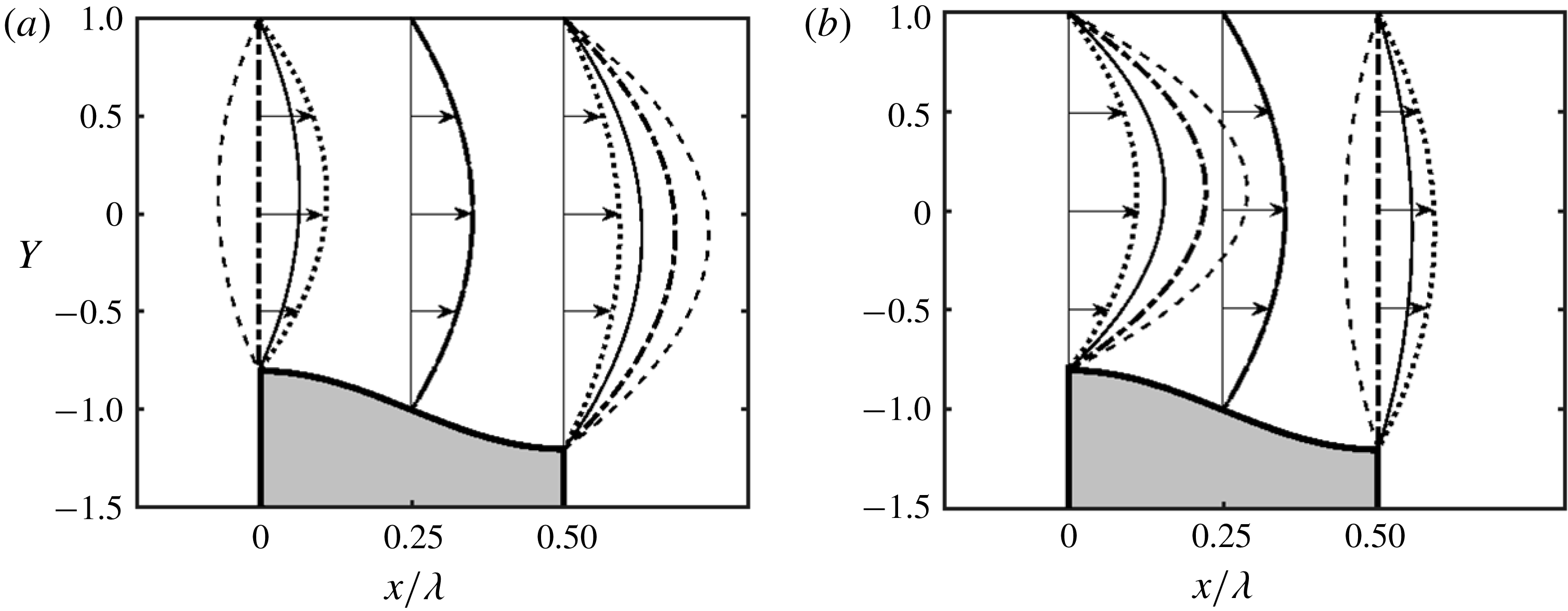
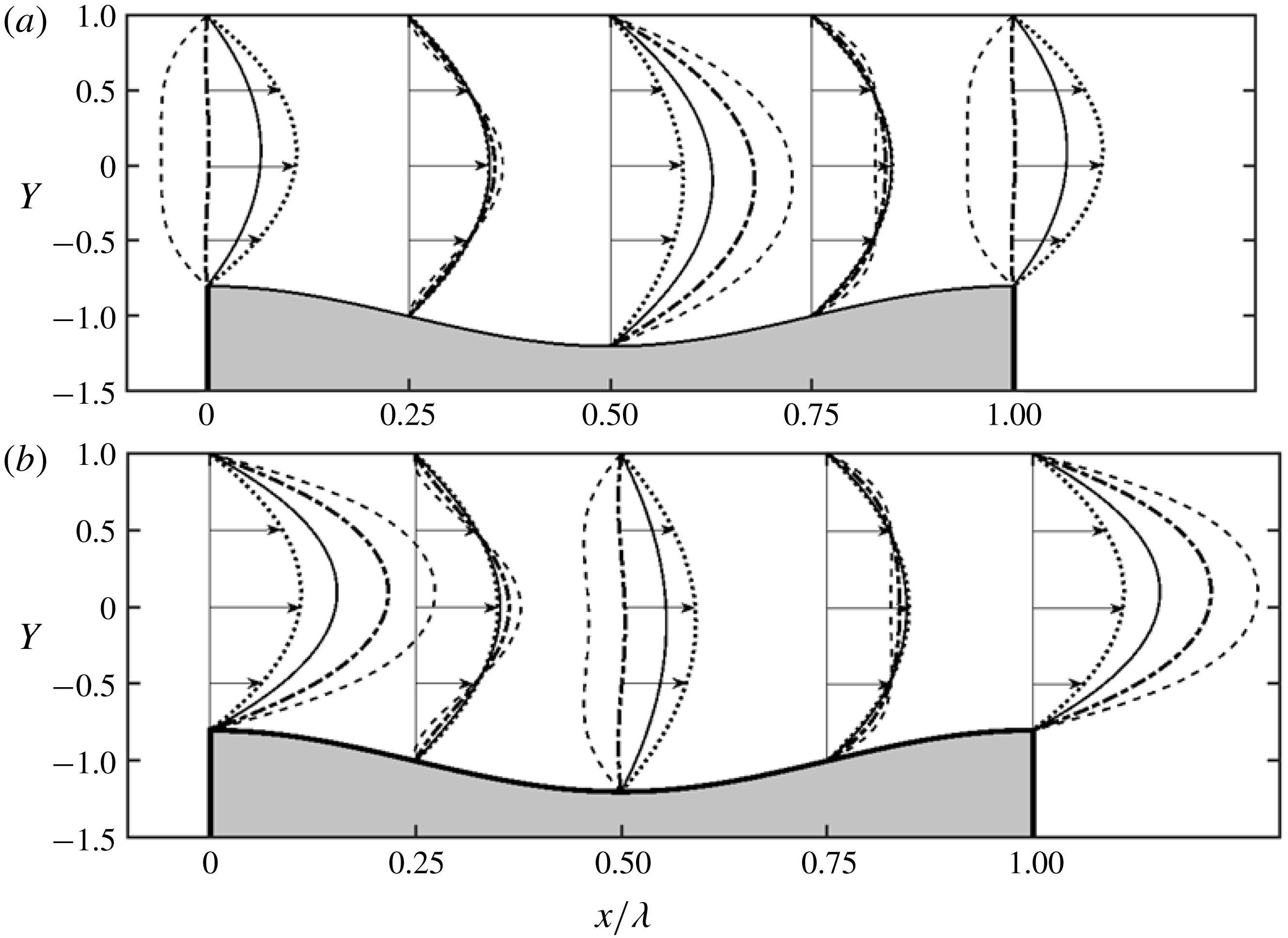
The change in the character of the velocity field is well illustrated by velocity distributions at the crests and troughs displayed in figure 4. When the wall is modified with stationary grooves (
 $c=0$
), the flow accelerates around the crest and slows down around the trough as dictated by changes in the flow cross-sectional area. When the waves propagate in the streamwise direction, the flow accelerates in the trough area and decelerates in the crest area with more pronounced effects for larger
 $c$
values. This suggests that the wave crest acts as a piston pushing fluid forward. When
 $c$
is large enough, the push is so strong that it creates a backflow around the troughs. Waves propagating upstream create an opposite effect with the flow accelerating at the crest and decelerating at the trough. Since the net flow rate must remain the same and the ‘piston’ is moving upstream, the fluid must accelerate at the crest to compensate for the reduced flow area and then must slow down at the trough due to the expansion of the flow area. Large enough
 $c$
leads to an expansion rapid enough to form a backflow at the trough.
Distributions of
 $u$
across the channel for
 $Re=1$
,
 $A=0.2$
and
 $\unicode[STIX]{x1D6FC}=0.01.$
(a) Displays data for the stationary grooves (
 $c=0$
, dotted line) and waves propagating downstream with
 $c=2.66$
(solid line),
 $6.66$
(dashed-dotted line) and 10.66 (dashed line). (b) Displays data for waves propagating upstream with
 $c=-2.66$
(solid line),
 $-6.66$
(dashed-dotted line) and
 $-10.66$
(dashed line); data for
 $c=0$
are added for reference. Data for the other half-wavelength are not shown due to the near mirror symmetry.

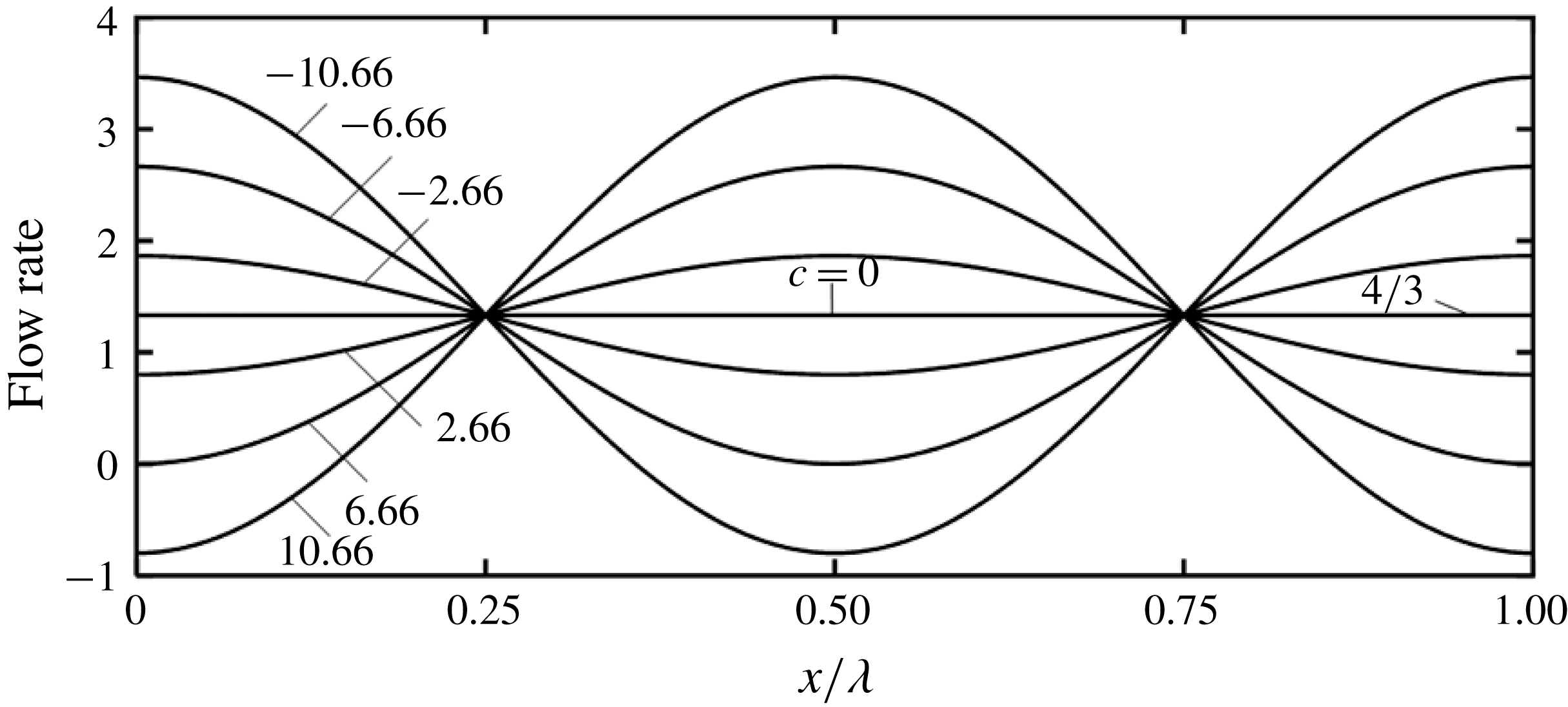
Distributions of the local flow rates presented in figure 5 provide another illustration of flow redistribution caused by the waves, i.e. concentration of flow in the trough areas for waves propagating downstream and in the crest areas for waves propagating upstream.
Variations of the flow rate along the channel for
 $A=0.2$
,
 $\unicode[STIX]{x1D6FC}=0.01$
and
 $Re=1$
, 100. Data for both
 $Re$
values overlap.

5 Forces created by the one-wall vibrations
Analysis of forces acting on the fluid starts with an expression for pressure written as a sum of the periodic
 $(p_{per})$
and aperiodic
 $(p_{aper})$
components, i.e.
 $$\begin{eqnarray}\displaystyle p & = & \displaystyle p_{per}+p_{aper}\nonumber\\ \displaystyle & = & \displaystyle \left\{\unicode[STIX]{x1D6FC}^{-1}\left[\tilde{p}_{-1}-Re^{-1}\left(1-\frac{A^{2}}{4}\right)^{-5/2}\left[-2\left(1+\frac{A^{2}}{8}\right)+\frac{9}{8}cA^{2}\right]\unicode[STIX]{x1D709}\right]+\tilde{p}_{0}+O(\unicode[STIX]{x1D6FC})\right\}\nonumber\\ \displaystyle & & \displaystyle +\,\left\{\unicode[STIX]{x1D6FC}^{-1}Re^{-1}\left(1-\frac{A^{2}}{4}\right)^{-5/2}\left[-2\left(1+\frac{A^{2}}{8}\right)+\frac{9}{8}cA^{2}\right]\unicode[STIX]{x1D709}+O(\unicode[STIX]{x1D6FC})\right\}.\end{eqnarray}$$
Since pressure is not a function of
 $\unicode[STIX]{x1D702}$
at this level of approximation and
 $\text{d}\tilde{p}_{0}/\text{d}\unicode[STIX]{x1D709}$
is purely periodic, the mean gradient is determined by
 $\tilde{p}_{-1}$
. Accordingly, this gradient can be written as
 $$\begin{eqnarray}\displaystyle Re\left.\frac{\text{d}p}{\text{d}X}\right|_{mean}=-2+ReB=-2\left(1-\frac{A^{2}}{4}\right)^{-5/2}\left(1+\frac{A^{2}}{8}-\frac{9}{16}cA^{2}\right)+O(\unicode[STIX]{x1D6FC}^{2}) & & \displaystyle\end{eqnarray}$$
which leads to a correction
 $B$
of the form
 $$\begin{eqnarray}\displaystyle B=\left.\frac{\text{d}p}{\text{d}X}\right|_{mean}+2Re^{-1}=Re^{-1}\left[-2\left(1-\frac{A^{2}}{4}\right)^{-5/2}\left(1+\frac{A^{2}}{8}-\frac{9}{16}cA^{2}\right)+2\right]+O(\unicode[STIX]{x1D6FC}^{2}). & & \displaystyle \nonumber\\ \displaystyle & & \displaystyle\end{eqnarray}$$
Since
 $A<2,B$
is negative in the absence of waves (
 $c=0$
), i.e. stationary grooves always increase drag. The pressure gradient is not affected (
 $B=0$
) by waves with the phase speed
 $$\begin{eqnarray}\displaystyle c_{n}=\frac{16}{9}A^{-2}\left[1+\frac{A^{2}}{8}-\left(1-\frac{A^{2}}{4}\right)^{5/2}\right], & & \displaystyle\end{eqnarray}$$
which we shall refer to as the neutral phase speed;
 $c_{n}$
is always positive and does not depend on
 $Re$
. Increase of
 $c$
above
 $c_{n}$
results in a reduction of the pressure gradient below that found in a stationary channel. The pressure gradient is decreased to zero by waves with the phase speed
 $$\begin{eqnarray}\displaystyle c_{cr}=\frac{16}{9}A^{-2}\left(1+\frac{A^{2}}{8}\right) & & \displaystyle\end{eqnarray}$$
which we shall refer to as the critical phase speed. This wave speed also does not depend on
 $Re$
. Use of waves with
 $c>c_{cr}$
requires use of a positive pressure gradient of order to prevent fluid from accelerating.
We shall now describe mechanisms responsible for changes of pressure gradient. Drag is generated only by shear when the channel is smooth. In the case of stationary corrugations (
 $c=0$
), both pressure and shear contribute to the drag increase. Pressure contributes through interaction with the surface topography while shear contributes through the increase of the wetted surface area and change of shear distribution (Mohammadi & Floryan Reference Mohammadi and Floryan2012, Reference Mohammadi and Floryan2013a
).
Surface waves (
 $c\neq 0$
) create a more complex situation. Evaluation of the
 $X$
-component of pressure force at the lower wall gives
 $$\begin{eqnarray}\displaystyle & & \displaystyle Ref_{X,pres}=ReA\sin (\unicode[STIX]{x1D709})[\tilde{p}_{-1}(\unicode[STIX]{x1D709})+\unicode[STIX]{x1D6FC}\tilde{p}_{0}(\unicode[STIX]{x1D709})+O(\unicode[STIX]{x1D6FC}^{2})]\nonumber\\ \displaystyle & & \displaystyle \quad =\left\{-A\sin (\unicode[STIX]{x1D709})\left(1-\frac{A^{2}}{4}\right)^{-5/2}\left(2+\frac{A^{2}}{4}-\frac{9}{8}cA^{2}\right)\unicode[STIX]{x1D709}\right\}\nonumber\\ \displaystyle & & \displaystyle \qquad +\left\{-3A^{2}\sin ^{2}(\unicode[STIX]{x1D709})\left(\!1-\frac{A^{2}}{4}\right)^{-5/2}\left[1-\frac{1}{2}c\left(\!1+\frac{A^{2}}{2}\right)\right]+\cdots +\unicode[STIX]{x1D6FC}ReA\sin (\unicode[STIX]{x1D709})\tilde{p}_{0}(\unicode[STIX]{x1D709})\!\right\}\nonumber\\ \displaystyle & & \displaystyle \qquad +\,O(\unicode[STIX]{x1D6FC}^{2})\nonumber\\ \displaystyle & & \displaystyle \quad =Ref_{X,form}+Ref_{X,inter}+O(\unicode[STIX]{x1D6FC}^{2}),\end{eqnarray}$$
where the first and second curly brackets lead to the form
 $(f_{X,form})$
and interaction
 $(f_{X,inter})$
drags (Mohammadi & Floryan Reference Mohammadi and Floryan2012), respectively. Substitution of (5.6) into (2.8) and evaluation of
 $F_{X,pres}$
show that terms omitted in (3.8) in the expression for
 $\tilde{p}_{-1}(\unicode[STIX]{x1D709})$
as well as the complete
 $\tilde{p}_{0}$
, do not contribute as integrals of
 $\sin (\unicode[STIX]{x1D709})\sin (n\unicode[STIX]{x1D709})$
with
 $n>1$
over one period are zero. The expression for
 $F_{X,pres}$
has the following form
 $$\begin{eqnarray}\displaystyle ReF_{X,pres} & = & \displaystyle Re(F_{X,form}+F_{X,inter})\nonumber\\ \displaystyle & = & \displaystyle \left\{A\left(1-\frac{A^{2}}{4}\right)^{-5/2}\left(2+\frac{A^{2}}{4}-\frac{9}{8}cA^{2}\right)\cos (\unicode[STIX]{x1D6FE})\hspace{-2.0pt}\right\}\nonumber\\ \displaystyle & & \displaystyle -\left\{\frac{3}{2}A^{2}\left(1-\frac{A^{2}}{4}\right)^{-5/2}\left[1-\frac{1}{2}c\left(1+\frac{A^{2}}{2}\right)\right]\hspace{-2.0pt}\right\}+O(\unicode[STIX]{x1D6FC}^{2}),\end{eqnarray}$$
where the first curly bracket captures the mean pressure gradient effect and is referred to as the form drag. This drag is a function of the segment of the wall being considered but, since it varies periodically with
 $\unicode[STIX]{x1D6FE}$
, it does not contribute to the overall drag. The second term captures the global effect and arises out of the interaction of the periodic part of
 $\tilde{p}_{-1}$
with the vibrating wall and is referred to as the interaction drag. This force initially opposes the fluid movement, but its magnitude is reduced through the increase of
 $c$
until it is eliminated when the phase speed reaches the critical value of
 $$\begin{eqnarray}\displaystyle c_{cr,pi}=4(A^{2}+2)^{-1}, & & \displaystyle\end{eqnarray}$$
which we shall refer to as the critical interaction speed;
 $c_{cr,pi}$
does not depend on
 $Re$
. Further increase of
 $c$
results in a change of direction of
 $F_{X,inter}$
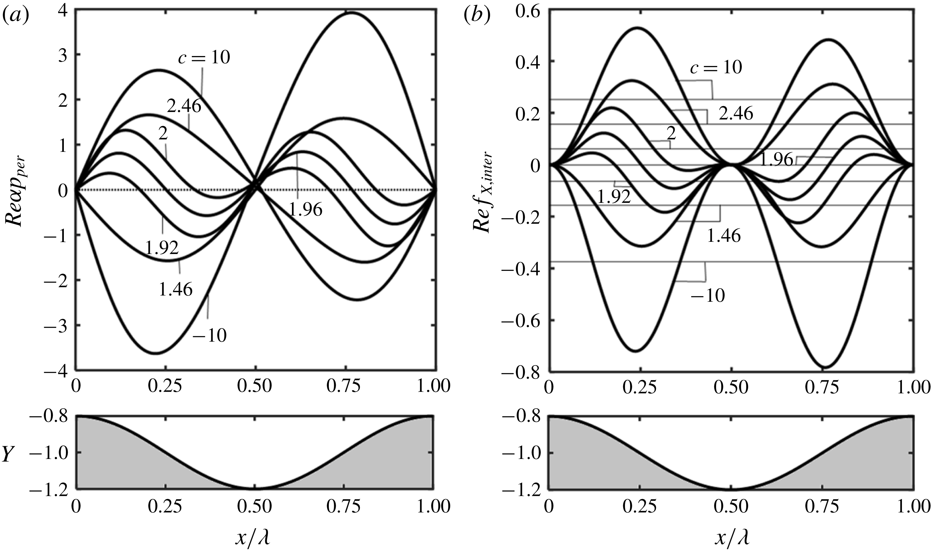
, i.e. this force begins to assist with the fluid movement. Distributions of
 $p_{per}$
displayed in figure 6(a) demonstrate a change of the relative position of the pressure field with respect to the wall geometry when
 $c$
crosses
 $c_{cr,pi}$
. When
 $c<c_{cr,pi}$
, the pressure at the wall is positive for
 $1<\unicode[STIX]{x1D709}/\unicode[STIX]{x03C0}<2$
and negative for
 $0<\unicode[STIX]{x1D709}/\unicode[STIX]{x03C0}<1$
opposing the fluid movement. When
 $c>c_{cr,pi}$
, the pressure is negative for
 $1<\unicode[STIX]{x1D709}/\unicode[STIX]{x03C0}<2$
and positive for
 $0<\unicode[STIX]{x1D709}/\unicode[STIX]{x03C0}<1$
supporting the fluid movement. Figure 6(b) displays distributions of the resulting
 $f_{X,inter}$
. The leading-order part of this force is positive everywhere for
 $c>c_{cr,pi}$
and negative everywhere for
 $c<c_{cr,pi}$
; contributions
 $O(\unicode[STIX]{x1D6FC})$
do not contribute to
 $F_{X,inter}$
so their variations are irrelevant.
Distributions of the periodic part of pressure
 $\unicode[STIX]{x1D6FC}p_{per}$
(a) and
 $f_{X,inter}$
(b) for
 $Re=1$
,
 $\unicode[STIX]{x1D6FC}=0.01$
,
 $A=0.2$
and
 $c=-10$
, 1.46, 1.92, 1.96, 2, 2.46, 10. Special values of
 $c$
for this case are
 $c_{n}=1.325$
,
 $c_{cr,pi}=1.96$
,
 $c_{cr}=44.66$
. In (b), thick and thin lines identify the local and mean values, respectively. Distributions and mean values for
 $c=1.46$
,
 $2.46$
have been multiplied by 10 for display purposes. Distributions and mean values for
 $c=1.92$
,
 $1.96$
,
 $2$
have been multiplied by 50 for display purposes.

We shall now look at viscous effects. Evaluation of the
 $X$
-component of shear stress acting at the lower wall gives
 $$\begin{eqnarray}\displaystyle Ref_{X,visc} & = & \displaystyle G_{1}^{-2}[-8+6cA\cos (\unicode[STIX]{x1D709})]\nonumber\\ \displaystyle & & \displaystyle +\,\unicode[STIX]{x1D6FC}ReG_{1}^{-1}\left\{\!{\textstyle \frac{32}{105}}A\sin (\unicode[STIX]{x1D709})G_{1}^{-1}-c\left[{\textstyle \frac{62}{105}}A^{2}\sin (2\unicode[STIX]{x1D709})G_{1}^{-1}\right.\right.\nonumber\\ \displaystyle & & \displaystyle +\left.A\left(-{\textstyle \frac{152}{105}}G_{1}^{-1}+{\textstyle \frac{16}{15}}\right)\sin (\unicode[STIX]{x1D709})\right]\nonumber\\ \displaystyle & & \displaystyle -\,c^{2}\left[-{\textstyle \frac{10}{7}}A^{3}\sin (3\unicode[STIX]{x1D709})G_{1}^{-1}+\left({\textstyle \frac{19}{35}}G_{1}^{-1}-{\textstyle \frac{7}{20}}\right)A^{2}\sin (2\unicode[STIX]{x1D709})\right.\nonumber\\ \displaystyle & & \displaystyle -\!\left.\left.{\textstyle \frac{1}{5}}A\sin (\unicode[STIX]{x1D709})\right]\!\right\}+O(\unicode[STIX]{x1D6FC}^{2}).\end{eqnarray}$$
The evaluation of the total viscous force through the substitution of (5.9) into (2.8) and integration shows that the term in the curly brackets in (5.9) does not contribute to this force, as it is an odd function of
 $\unicode[STIX]{x1D709}$
, resulting in the expression for
 $F_{X,visc}$
of the form
 $$\begin{eqnarray}\displaystyle ReF_{X,visc}=\left(1-\frac{A^{2}}{4}\right)^{-3/2}\left(-2+c\frac{3}{4}A^{2}\right)+O(\unicode[STIX]{x1D6FC}^{2}). & & \displaystyle\end{eqnarray}$$
The above relation demonstrates that the increase of
 $c$
reduces
 $F_{X,visc}$
until it reaches zero at
 $$\begin{eqnarray}\displaystyle c_{cr,v}={\textstyle \frac{8}{3}}A^{-2}, & & \displaystyle\end{eqnarray}$$
which we shall refer to as the critical viscous speed. Further increase of
 $c$
changes the direction of
 $F_{X,visc}$
which now pushes the fluid in the positive
 $X$
-direction. It is interesting to note that
 $c_{cr,v}$
is never smaller than
 $2/3$
and that a smaller
 $A$
leads to a larger
 $c_{cr,v}$
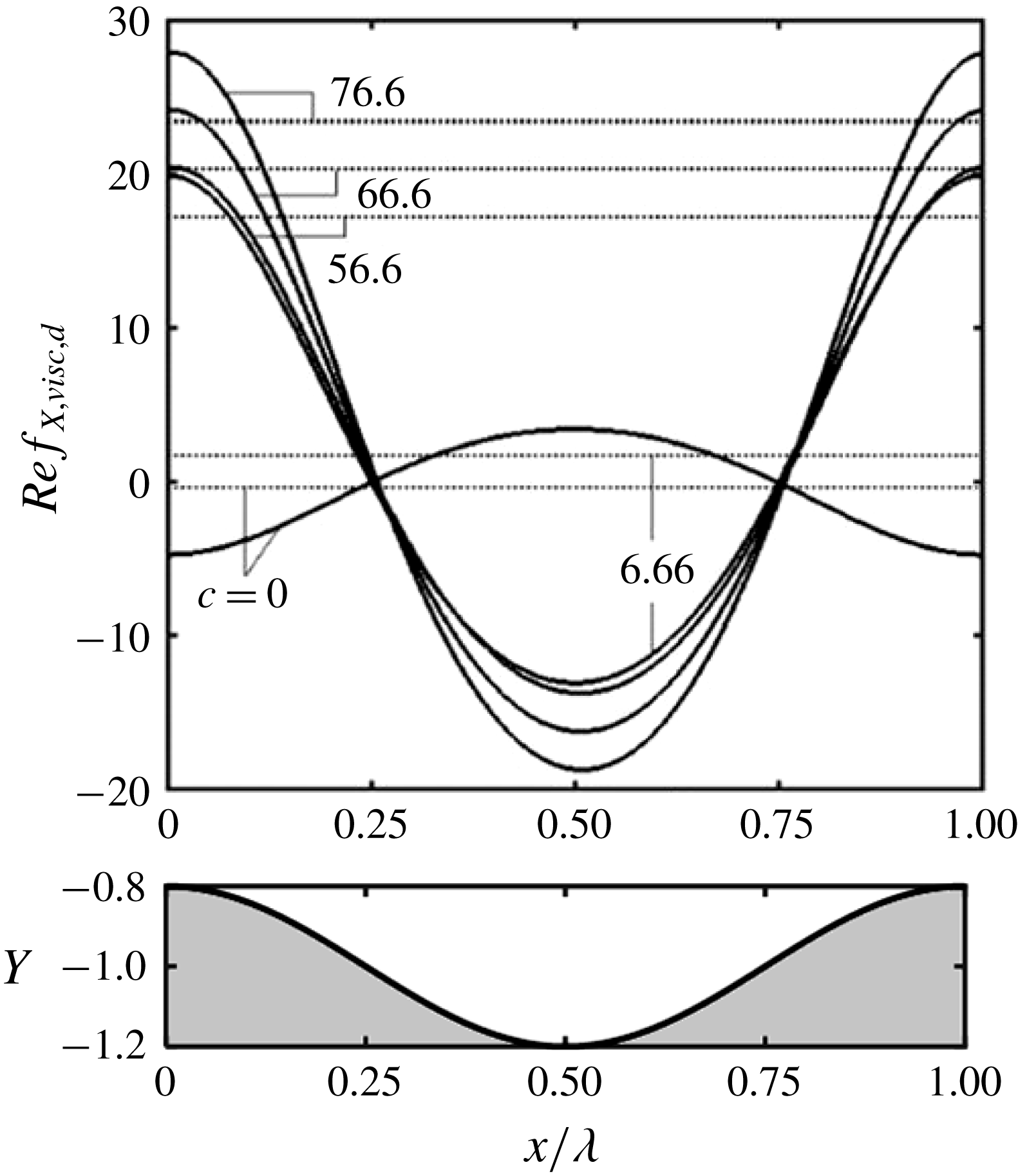
. Distributions of the difference between the shear stresses in the vibrating and smooth channels, i.e.
 $f_{X,visc,d}=f_{X,visc}+2/Re$
, displayed in figure 7 have approximately cosine forms but the amplitudes are much larger than the stress in the smooth channel and increase together with their mean values
 $(f_{X,visc,d,mean})$
when
 $c$
increases. Nothing unusual happens at
 $c=c_{cr,v}$
; the size of the separation zone smoothly increases with
 $c$
until the wall shear in the separation zone becomes large enough so that the shear force reverses its direction.
Distributions of viscous forces acting on the fluid at the lower wall for
 $A=0.2$
,
 $Re=1$
. Solid and dotted lines identify the local
 $(f_{X,visc,d})$
and mean
 $(f_{X,visc,d,m})$
values, respectively. Special values of
 $c$
for this case are
 $c_{sep}=6.66$
,
 $c_{cr,v}=66.6$
. Local values for
 $c=0,6.66$
as well as all mean values have been multiplied by 10 for display purposes.

The determination of the
 $X$
-component of shear acting at the upper wall follows a similar process and demonstrates that
 $g_{X,visc}$
and
 $G_{X,visc}$
are the same as at the lower wall, i.e.
 $g_{X,visc}=f_{X,visc}$
,
 $G_{X,visc}=F_{X,visc}$
and separation occurs under the same conditions and at the same locations. The pressure forces do not produce any
 $X$
-component at the upper wall, i.e.
 $g_{X,pres}=0$
and
 $G_{X,pres}=0$
.
The sum of
 $F_{X,visc}$
,
 $G_{X,visc}$
and
 $F_{X,inter}$
gives the
 $X$
-component
 $H_{X,tot}$
of the total force
 $H_{tot}$
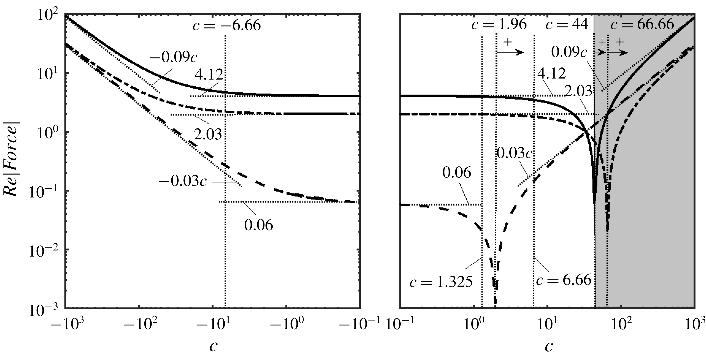
. Variations of
 $H_{X,tot}$
as well as its components as functions of the phase speed illustrated in figure 8 show that there are three ranges of
 $c$
. In the first one, both pressure and viscous forces oppose the fluid movement. The increase of
 $c$
leads to the second range where the pressure forces contribute to the driving force while viscous forces oppose it. Further increase of
 $c$
leads to the third range where both the pressure and viscous forces contribute to the driving force. It is worth observing that forces for sufficiently large positive
 $c$
values and sufficiently large negative
 $c$
values have the same magnitudes but opposite directions.
Detailed analysis of
 $H_{X,tot}$
shows that the external pressure gradient required to drive the flow decreases when
 $c$
increases until it reaches zero when
 $H_{X,tot}\approx 4/Re$
. This condition defines properties of waves which produce a propulsive effect equivalent to the external pressure gradient. When
 $H_{X,tot}\,>\sim 4/Re$
, the vibrations are strong enough so that the external pressure gradient must reverse direction to prevent fluid from accelerating. Such conditions can be easily achieved and correspond to the grey shading in figure 8. The corresponding waves have the same or better pumping abilities as the external pressure gradient and, thus, data presented in figure 8 may be used to define pumping equivalence between vibrations and the external pressure gradient.
Variations of
 $H_{X,tot}$
(solid line),
 $F_{X,visc}$
(dashed-dotted line) and
 $F_{X,inter}$
(dashed line) as functions of
 $c$
for
 $A=0.2$
. The special wave speeds are:
 $c_{n}=1.325$
,
 $c_{cr}=44.66$
,
 $c_{cr,pi}=1.96$
,
 $c_{cr,v}=66.6$
,
 $c_{sep}=6.66$
. The grey zone identifies
 $c$
values where the pressure gradient needs to change direction to prevent fluid from accelerating.

Variations of different critical phase speeds as functions of
 $A$
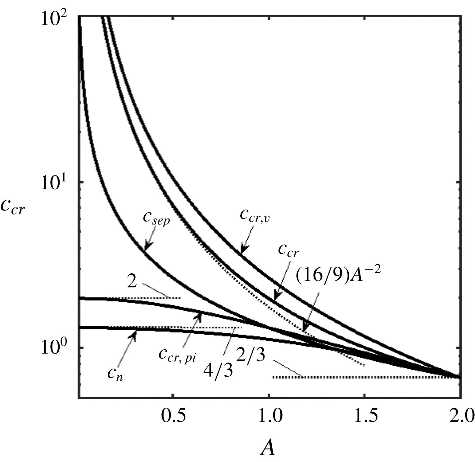
are illustrated in figure 9. These speeds are never smaller than
 $2/3$
,
 $c_{cr}$
and
 $c_{cr,v}$
increase without bounds when
 $A\rightarrow 0$
while
 $c_{cr,pi}$
approaches a limit point of 2;
 $A=0$
represents another limit point at which
 $c$
plays no role. Waves with small
 $c$
values generate pressure force pushing fluid in the positive
 $X$
-direction while faster waves are required to overcome friction and reduce the pressure gradient to zero. The difference between both critical phase speeds decreases as
 $A\rightarrow 2$
.
Variations of the special phase speeds
 $c_{n},c_{cr},c_{cr,v},c_{cr,pi},c_{sep}$
as functions of the amplitude
 $A$
.

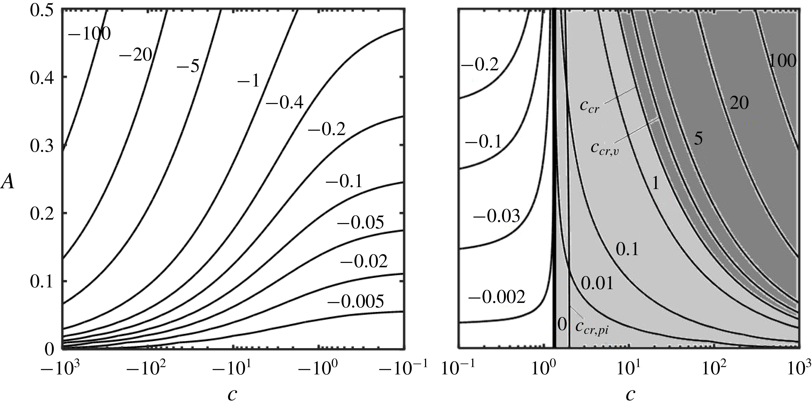
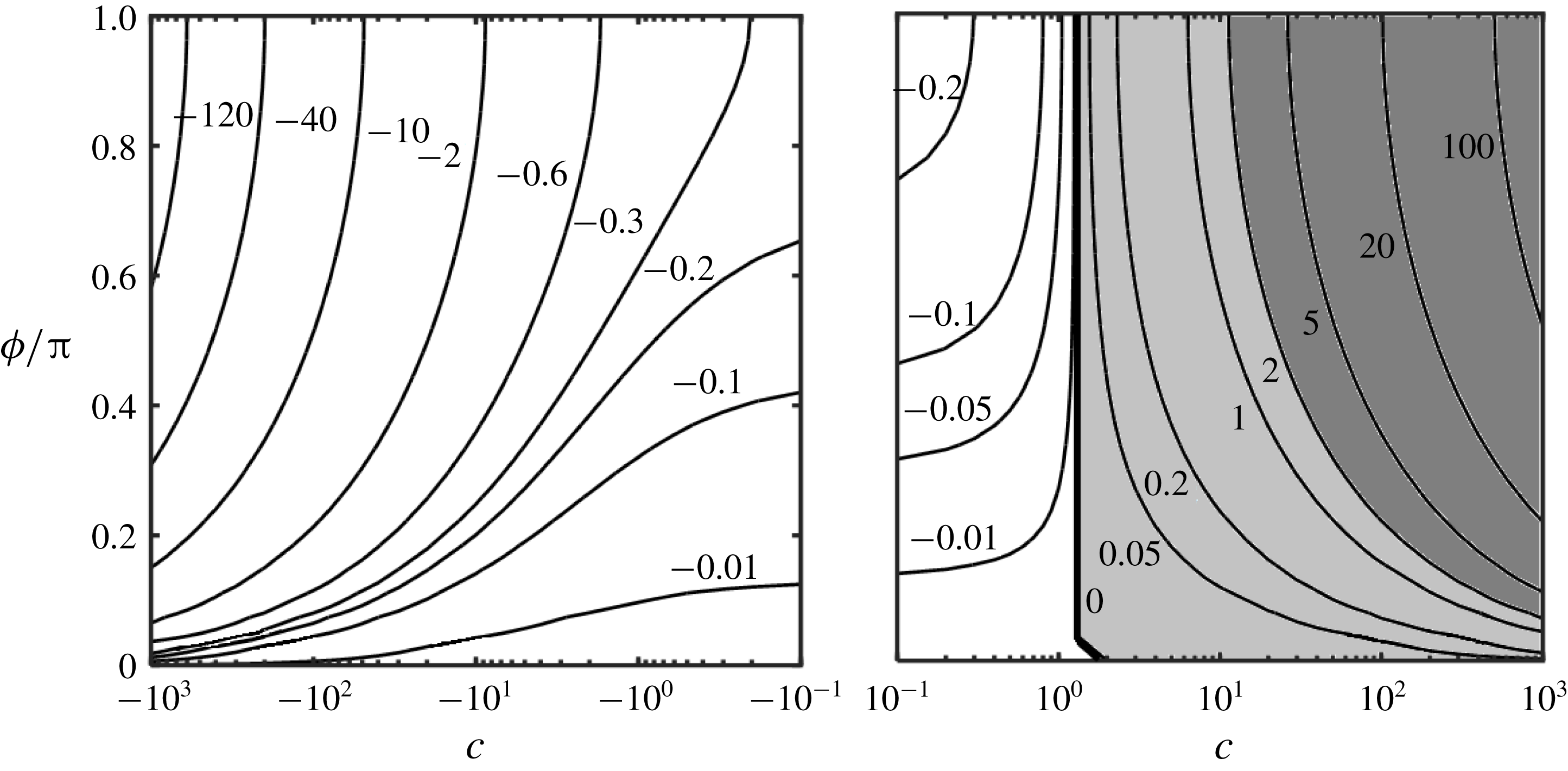
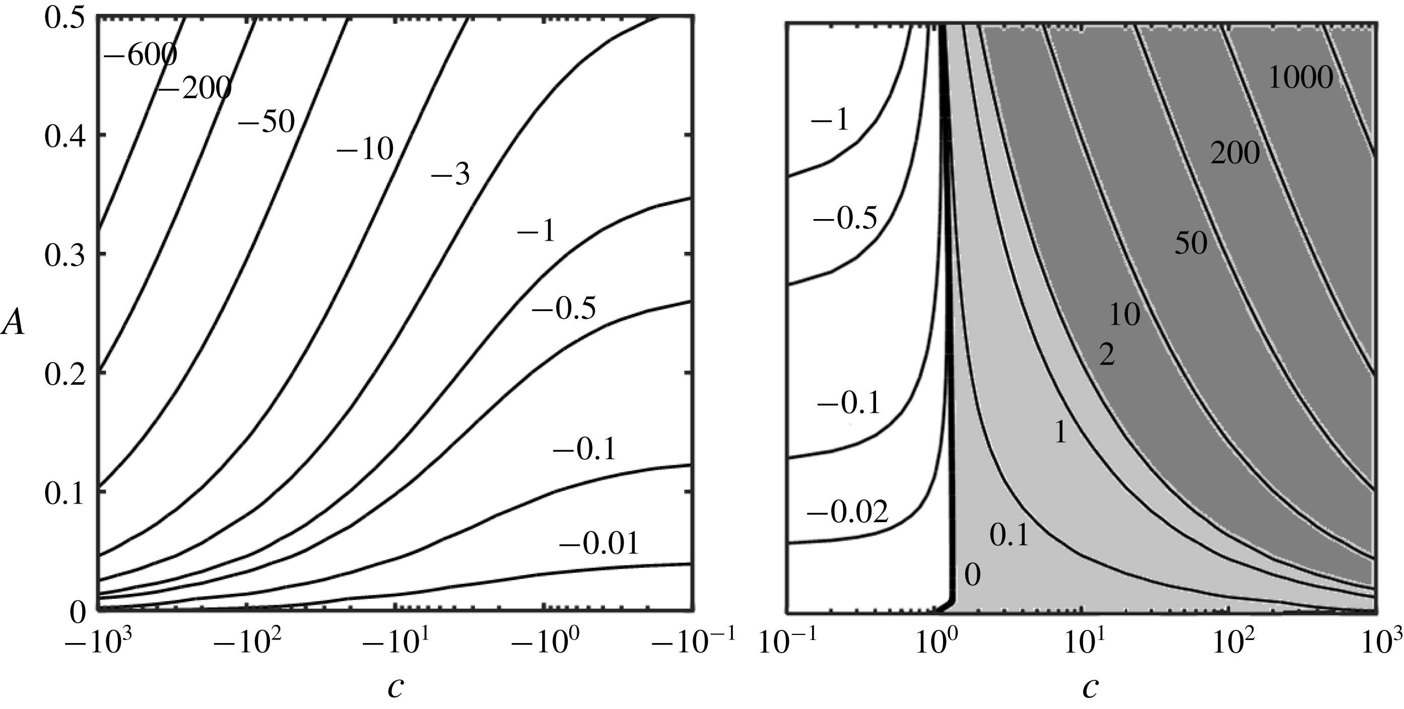
Figure 10 illustrates changes of the pressure gradient correction
 $ReB$
for a wide range of variations of
 $c$
and for
 $A$
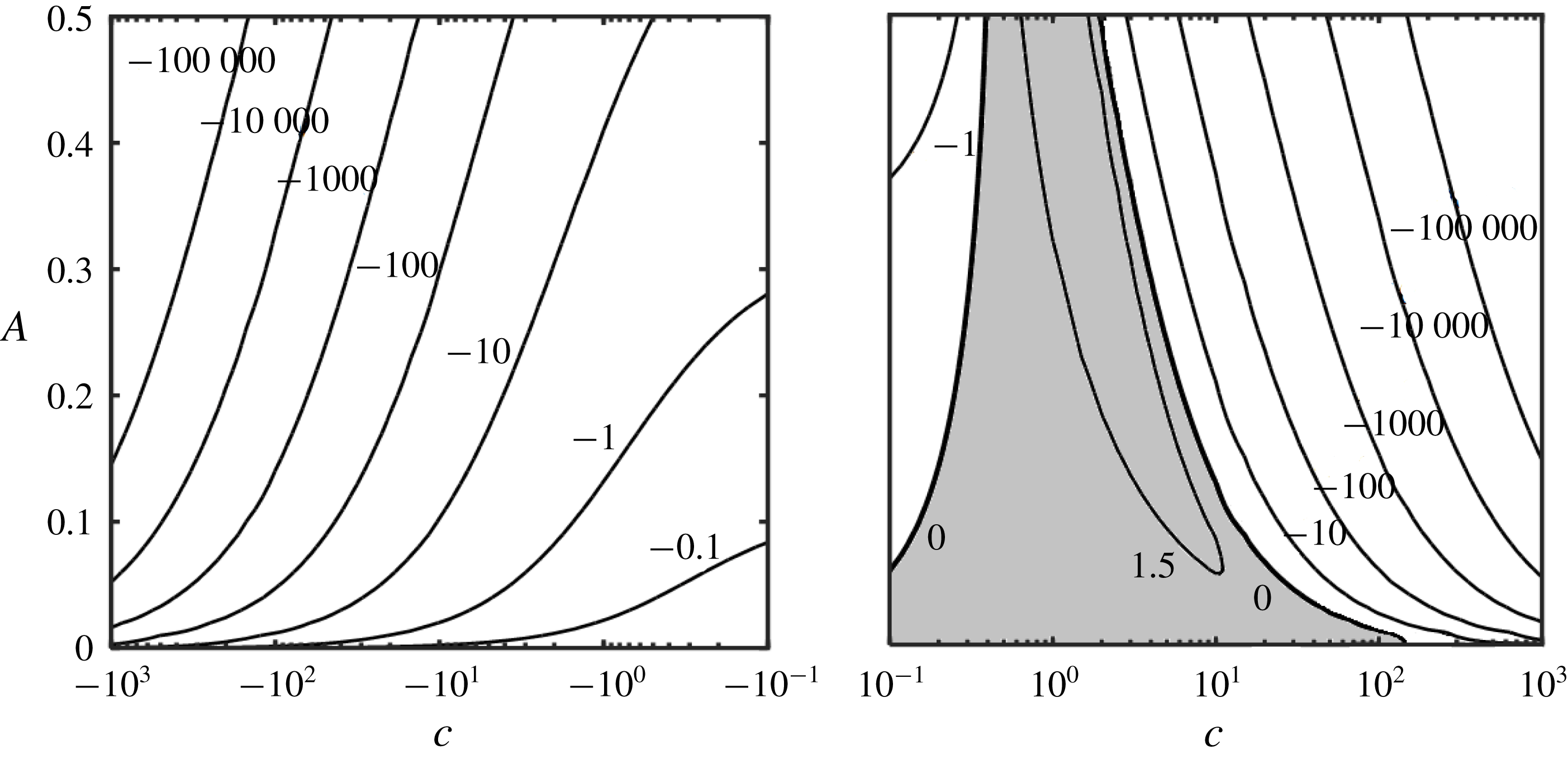
values extending up to 25 % of the channel opening. There is a clear trend of
 $ReB$
increasing with an increase of positive
 $c$
and decreasing with an increase of negative
 $c$
, and increasing with an increase of
 $A$
.
Variations of the pressure gradient correction
 $ReB$
as a function of
 $c$
and
 $A$
. The light shaded area identifies conditions leading to a reduction of the pressure gradient while the dark shaded are identifies conditions where the pressure gradient must change direction to maintain the same flow rate.

Analysis of forces acting in the
 $Y$
-direction begins with the determination of
 $f_{Y,visc}$
, i.e.
 $$\begin{eqnarray}\displaystyle Ref_{Y,visc}=\unicode[STIX]{x1D6FC}AG_{1}^{-2}[8\sin (\unicode[STIX]{x1D709})-c3A\sin (2\unicode[STIX]{x1D709})]+O(\unicode[STIX]{x1D6FC}^{2}). & & \displaystyle\end{eqnarray}$$
Integration of (5.12) over one wavelength demonstrates that
 $F_{Y,visc}=O(\unicode[STIX]{x1D6FC}^{2})$
. The
 $Y$
-component generated by the pressure has the form
 $$\begin{eqnarray}\displaystyle Ref_{Y,pres}=Re[\unicode[STIX]{x1D6FC}^{-1}\tilde{p}_{-1}(\unicode[STIX]{x1D709})+\tilde{p}_{0}(\unicode[STIX]{x1D709})+O(\unicode[STIX]{x1D6FC})]. & & \displaystyle\end{eqnarray}$$
Substitution of (3.8) and (3.10d
) into (5.13) and use of (2.8) show that only terms linear in
 $\unicode[STIX]{x1D709}$
from
 $\tilde{p}_{-1}$
and
 $\tilde{p}_{0}$
bring non-zero contributions, i.e.
 $$\begin{eqnarray}\displaystyle ReF_{Y,pres} & = & \displaystyle -\unicode[STIX]{x1D6FC}^{-1}2(\unicode[STIX]{x1D6FE}+\unicode[STIX]{x03C0})\left(1-\frac{A^{2}}{4}\right)^{-5/2}\left(1+\frac{A^{2}}{8}-c\frac{9}{16}A^{2}\right)\nonumber\\ \displaystyle & & \displaystyle -\,\frac{12}{35}Re\left[\left(1-\frac{A^{2}}{4}\right)^{-3/2}-\left(1-\frac{A}{2}\right)^{-2}\right]\nonumber\\ \displaystyle & & \displaystyle +\,c\frac{2}{35}Re\left[\left(16+\frac{A^{2}}{2}\right)\left(1-\frac{A^{2}}{4}\right)^{-3/2}-(16+A)\left(1-\frac{A}{2}\right)^{-2}\right]\nonumber\\ \displaystyle & & \displaystyle -\,c^{2}\frac{3}{35}Re\left\{\left(7+\frac{A^{2}}{2}\right)\left(1-\frac{A^{2}}{4}\right)^{-3/2}-(7+A)\left(1-\frac{A}{2}\right)^{-2}\right.\nonumber\\ \displaystyle & & \displaystyle +\left.2\ln \left[\left(1+\left(1-\frac{A^{2}}{4}\right)^{1/2}\right)(2-A)^{-1}\right]\right\}+O(\unicode[STIX]{x1D6FC}).\end{eqnarray}$$
The effect of vibrations is better judged by looking at the difference
 $F_{Y,pres,d}$
between forces in vibrating and smooth channels, i.e.
 $$\begin{eqnarray}\displaystyle ReF_{Y,pres,d}=ReF_{Y,pres}+\unicode[STIX]{x1D6FC}^{-1}2(\unicode[STIX]{x1D6FE}+\unicode[STIX]{x03C0}). & & \displaystyle\end{eqnarray}$$
Comparisons between various forms of vibrations can be made using the same channel segment which, in this discussion, always corresponds to
 $\unicode[STIX]{x1D6FE}=0$
. The direction of
 $F_{Y,pres,d}$
depends on
 $c$
, e.g. when
 $A=0.2$
,
 $Re=1$
,
 $\unicode[STIX]{x1D6FC}=0.01$
,
 $\unicode[STIX]{x1D6FE}=0$
,
 $F_{Y,pres,d}$
is negative for
 $-108.38<c<1.32$
and positive otherwise. This shows that the slow forward and relatively fast backward waves produce force acting in the negative
 $Y$
-direction while the fast forward waves and very fast backward waves produce force acting in the positive
 $Y$
-direction. Pressure force in the
 $Y$
-direction at the upper wall is equal and opposite to the pressure force at the lower wall, i.e.
 $G_{Y,pres}=-F_{Y,pres}$
. The directions of the
 $Y$
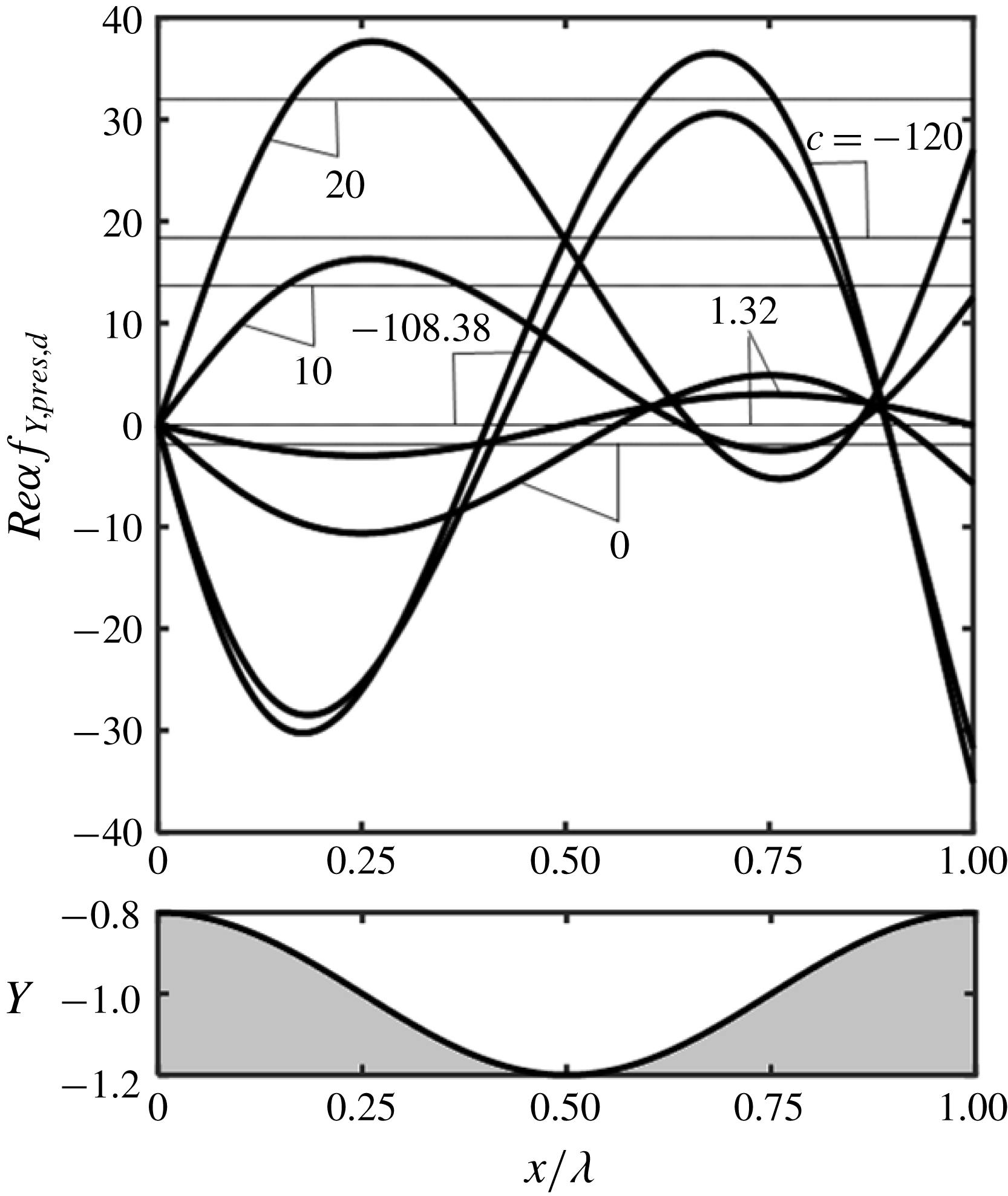
-forces demonstrate that fast enough forward and backward waves produce a compressing effect. Distributions of the difference between the local pressure forces in the vibrating and smooth channels, i.e.
 $f_{Y,pres,d}=f_{Y,pres}+2\unicode[STIX]{x1D6FC}^{-1}Re^{-1}\unicode[STIX]{x1D709}$
, displayed in figure 11 show a large range of variation over a single wavelength. Waves moving in the flow direction produce a large force increase on the forward face and a small decrease on the backward face while waves moving in the upstream direction produce significant reduction on the forward face and an increase of the backward face. The local changes are an order of magnitude larger than the mean values.
Distributions of
 $f_{Y,pres,d}$
for
 $A=0.2$
,
 $Re=1$
,
 $\unicode[STIX]{x1D6FE}=0$
and
 $c=-120,-108.38,0,1.32,10,20$
. Thick and thin lines identify the local and mean values, respectively. Local values for
 $c=10,20$
have been multiplied by
 $5$
and local values for
 $c=0,1.32$
have been multiplied by
 $15$
. All mean values have been multiplied by
 $10$
for display purposes.

We shall now turn our attention to analysis of the actuation power. The
 $Y$
-component of the surface forces has contributions from the pressure and viscous forces creating pressure actuation power
 $({\wp}_{act,p})$
and viscous actuation power
 $({\wp}_{act,v})$
, and leading to the total actuation power of the form
 $$\begin{eqnarray}\displaystyle {\wp}_{act}={\wp}_{act,v}+{\wp}_{act,p}. & & \displaystyle\end{eqnarray}$$
The viscous power can be computing by substituting
 $f_{Y,visc}$
from (2.6b
) into (2.11) and carrying out the required integration to arrive at
 $$\begin{eqnarray}\displaystyle {\wp}_{act,v}=O(\unicode[STIX]{x1D6FC}^{2}), & & \displaystyle\end{eqnarray}$$
which demonstrates that viscous contributions are negligible. The pressure power can be computed in the same manner by substituting
 $f_{Y,pres}$
from (2.6b
) into (2.11) to carrying out integrations to arrive at
 $$\begin{eqnarray}\displaystyle Re{\wp}_{act,p}=\frac{Ac}{2}\left(1-\frac{A^{2}}{4}\right)^{-5/2}\left[4-3A+\frac{A^{2}}{2}+cA\left(\frac{3}{2}-\frac{9}{4}A+\frac{3}{4}A^{2}\right)\right]+O(\unicode[STIX]{x1D6FC}^{2}).\qquad & & \displaystyle\end{eqnarray}$$
This power has two components, one associated with the mean pressure gradient
 $({\wp}_{act,p,mean})$
and the other one with the periodic pressure component
 $({\wp}_{act,p,per})$
. It can be shown that
 $$\begin{eqnarray}\displaystyle & \displaystyle Re{\wp}_{act,p,mean}=2Ac\left(1-\frac{A^{2}}{4}\right)^{-5/2}\left(1+\frac{A^{2}}{8}-\frac{9}{16}A^{2}c\right)=-ReAc\left.\frac{\text{d}p}{\text{d}x}\right|_{mean},\qquad & \displaystyle\end{eqnarray}$$
 $$\begin{eqnarray}\displaystyle & \displaystyle Re{\wp}_{act,p,per}=\frac{A^{2}c}{2}\left(1-\frac{A^{2}}{4}\right)^{-5/2}\left[-3+\frac{3}{2}c\left(1+\frac{A^{2}}{2}\right)\right]. & \displaystyle\end{eqnarray}$$
It is convenient to start discussion by looking at the effects of the mean pressure gradient, which are captured by (5.17c
). The negative pressure gradient leads to a positive actuation power for the downstream-propagating waves but negative power (energy savings) for the upstream-propagating waves; the situation is reversed for the positive pressure gradient. While the pressure gradient is not known a priori, results displayed in figure 10 show that the positive pressure gradient correction for the fast forward waves is large enough to make
 $\text{d}p/\text{d}x|_{mean}$
positive, which leads to the negative actuation power, and it is negative for the fast backward waves, which keeps
 $\text{d}p/\text{d}x|_{mean}$
negative, also resulting in the negative actuation power. Similar conclusions can be reached without relying on the direction of pressure gradient as the middle term of (5.17c
) shows that the actuation power is always negative for fast waves. Slower waves with
 $c=O(1)$
require energy input when propagating downstream but the actuation power is negative when such waves propagate upstream.
The effect of the periodic pressure field is obvious for large
 $|c|$
as the actuation power is always positive (see (5.17d
)). For
 $|c|=O(1)$
, the direction of energy flow is difficult to predict due to change in the relative position of the periodic pressure field and the wave crests, as illustrated in figure 6(a). Determination of the net effect involving both mechanisms requires detailed calculations as they oppose each other for large
 $|c|$
but change in a different manner for small
 $|c|$
. Data displayed in figure 12 illustrate the outcome of this competition and identify conditions where
 ${\wp}_{act,p}$
is negative.
Variations of
 $Re{\wp}_{act,p}$
,
 $Re{\wp}_{act,p,mean}$
and
 $Re{\wp}_{act,p,per}$
as functions of
 $c$
and
 $A$
. Solid, dashed, and dotted lines correspond to
 ${\wp}_{act,p}$
,
 ${\wp}_{act,p,mean}$
and
 ${\wp}_{act,p,per}$
, respectively. The grey zone identifies area where
 ${\wp}_{act,p}<0$
.

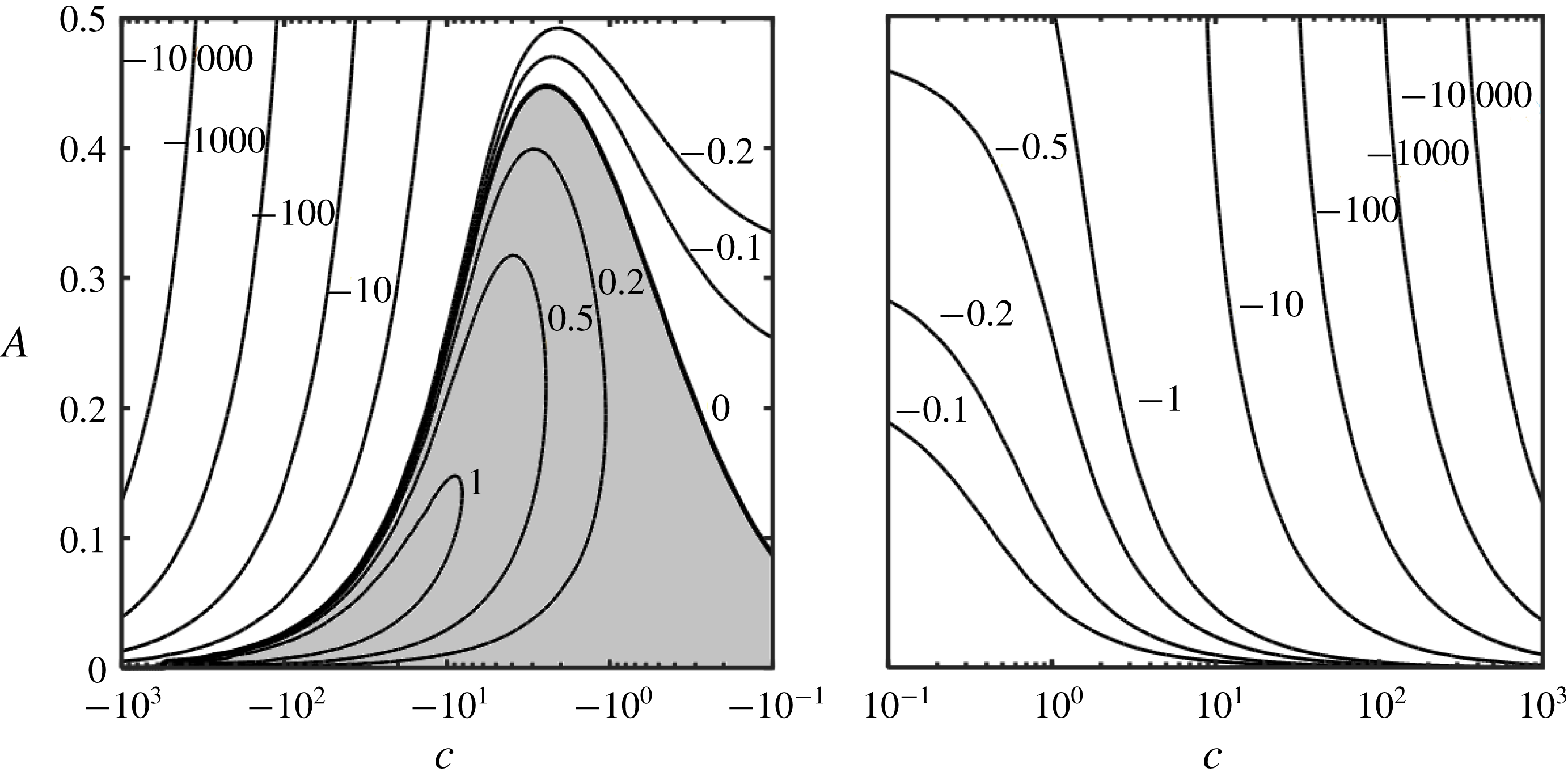
The net energy savings
 $\unicode[STIX]{x0394}{\wp}_{net}$
can be evaluated using (2.12) and (5.17), i.e.
 $$\begin{eqnarray}\displaystyle Re\unicode[STIX]{x0394}{\wp}_{net} & = & \displaystyle Re\unicode[STIX]{x0394}{\wp}_{net}=\frac{8}{3}-\left(1-\frac{A^{2}}{4}\right)^{-5/2}\left[\frac{8}{3}\left(1+\frac{A^{2}}{8}\right)\right.\nonumber\\ \displaystyle & & \displaystyle +\left.\frac{Ac}{2}\left(4-6A+\frac{A^{2}}{2}\right)+\frac{c^{2}A^{2}}{2}\left(\frac{3}{2}-\frac{9}{4}A+\frac{3}{4}A^{2}\right)\right].\end{eqnarray}$$
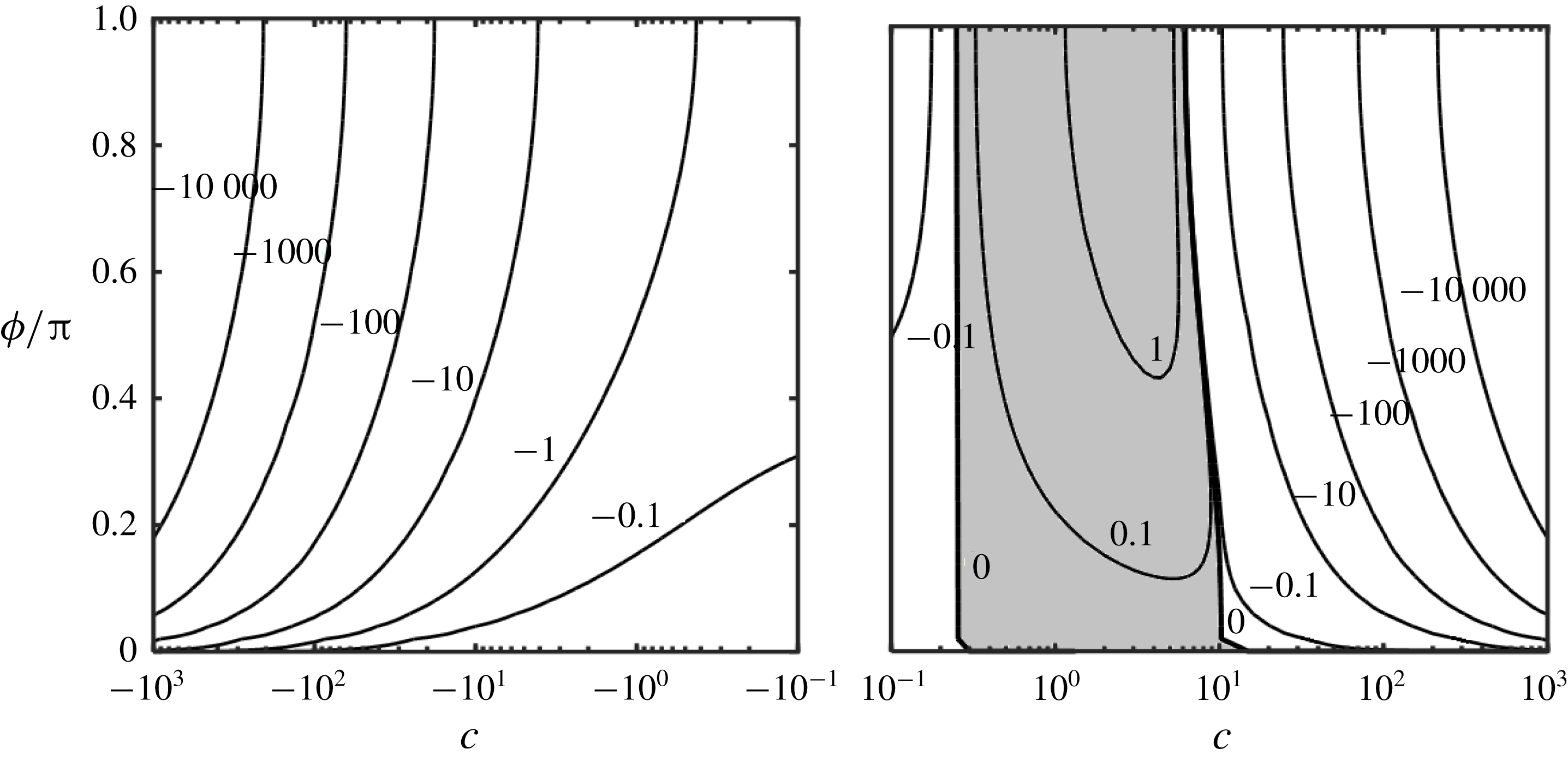
The savings are always negative for the fast waves regardless of the direction of propagation, i.e. such waves require a net addition of energy to the system. Variations of
 $\unicode[STIX]{x0394}{\wp}_{net}$
displayed in figure 13 demonstrate however that there exist a range of waves capable of extracting energy from the flow. These are upstream propagating waves with a wide range of phase speeds. Surprisingly, waves with smaller amplitudes are more effective. Such waves could be used for energy extraction from the flow. Waves propagating downstream always require net energy input in spite of the reduction of pressure gradient.
Variations of the energy savings
 $Re\unicode[STIX]{x0394}{\wp}_{net}$
as a function of
 $c$
and
 $A$
. The grey zone identifies conditions resulting in waves extracting energy from the flow.

6 Effects of the Reynolds number on the one-wall vibrations
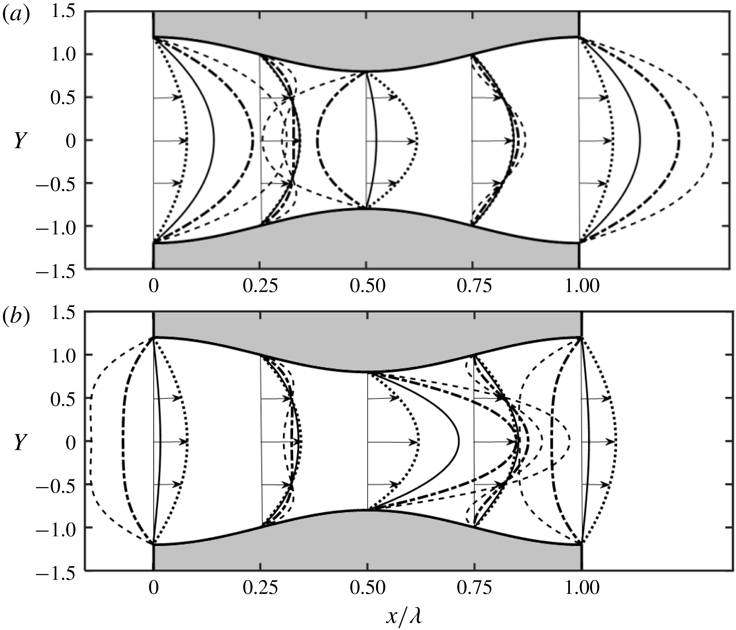
We begin the presentation by discussing changes in the velocity field resulting from the increase of
 $Re$
. Figure 14 displays such fields and figure 15 displays
 $u$
-velocity distributions for the same
 $c$
as in figures 2 and 4 but with the Reynolds number increased to
 $Re=100$
. The locations of the separation points remain unchanged. The flow patterns are nearly the same for both
 $Re$
values for
 $c=0$
(compare figures 2
d and 14
d). Increase of
 $c$
increases velocity in the trough area and decreases it in the crest area where the flow reversal takes place if the waves are fast enough (see figures 14
d–g and 15
a). There is a characteristic difference between the slow-down on the upstream side of the wave and acceleration of the downstream side, resulting in an asymmetry of velocity profiles (see figure 15). The slow-down between the trough and the crest begins in the middle of the channel resulting in a flattening of velocity profile which is more pronounced for larger
 $c$
(see velocity distribution for
 $c=10.66$
at
 $X/\unicode[STIX]{x1D706}=0.75$
in figure 15
b). The fluid acceleration between the crest and the trough also begins in the middle of the channel but results in the formation of a ‘jet’-like structure, with the ‘jets’ being more pronounced for larger
 $c$
(see figure 15
a). The backflow zone in the crest area forming for large enough
 $c$
has a characteristic crescent shape bending in the downstream direction (see figure 14
a). When the waves propagate in the opposite direction, the largest acceleration takes place in the crest area and deceleration in the trough area where the flow reverses direction if
 $|c|$
is large enough (see figures 14
a–d and 15
b). There is a characteristic flattening of velocity profiles above the downstream side of the wave and formation of the ‘jet’-like structures in the channel centre in the upstream side (see figure 15
b). The zone with the backflow has a characteristic crescent shape bending in the upstream direction (see figure 14
g). The differences in the velocity distributions at different
 $X$
-locations do not however affect the local flow rates (see figure 5).
Plots of velocity fields for
 $Re=100$
,
 $A=0.2$
,
 $\unicode[STIX]{x1D6FC}=0.01$
and
 $c=-10.66,-6.66,-2.66,0,2.66,6.66,10.66$
in (a–g), respectively. Shaded areas identify zones with reverse flow direction.

Distributions of
 $u$
across the channel for
 $Re=100$
,
 $A=0.2$
and
 $\unicode[STIX]{x1D6FC}=0.01.$
(a) Displays data for the stationary grooves (
 $c=0$
, dotted line) and waves propagating downstream with
 $c=2.66$
(solid line),
 $6.66$
(dashed-dotted line) and 10.66 (dashed line). (b) Displays data for waves propagating upstream with
 $c=-2.66$
(solid line),
 $-6.66$
(dashed-dotted line) and
 $-10.66$
(dashed line); data for
 $c=0$
are added for reference.

It has been shown that the surface waves propagating downstream are able to reduce the drag in the case of turbulent flow (Nakanishi et al. Reference Nakanishi, Mamori and Fukagata2012). The relevant Reynolds numbers are vastly different from those used in the present analysis but the velocity profiles displayed in figure 15 offer hints which could assist in the search for the most effective waves. The proper identification of the most promising waves is important as analysis of turbulent flows relies on DNS and the range of parameters to be investigated is just too wide to make complete search practical. Velocity profiles shown in figure 15(a) demonstrate small flow sensitivity to the waves in the areas half-way between the troughs and the crests, reduction of the wall shear around the crests and its increase in the trough area. It may be possible to identify waves whose shear reduction in the crest area outweighs shear increase in the trough area. The large changes of the average velocity between these two areas may lead to the local flow laminarization which would further contribute to the drag reduction. The above results suggest that the required waves should have high phase speeds which, in addition, will increase dissipation and reduce the intensity of turbulent fluctuations contributing to the further reduction of pressure losses.
The total forces acting on the fluid in the
 $X$
-direction are proportional to
 $Re$
as demonstrated by (5.7) and (5.10), and the characteristic phase velocities identified in §§ 4 and 5 remain unchanged. The surface stresses exhibit a more complex dependence as their distributions change with
 $Re$
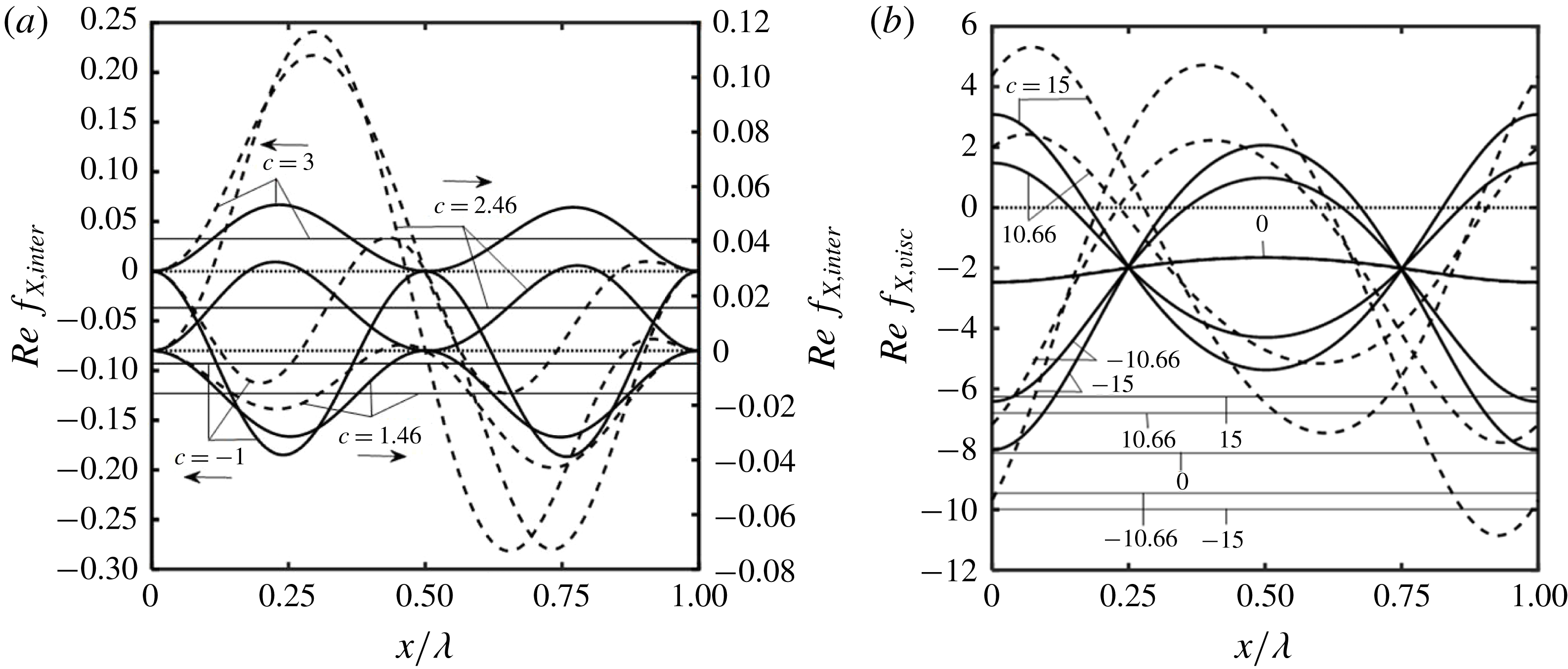
. The change is quite pronounced for pressure forces illustrated in figure 16(a) as the symmetry between the upstream and downstream sides is lost. Moreover, when
 $c>c_{cr,pi}$
, the forward face produces a large positive force while the rear face produces a large negative force. When
 $c<c_{cr,pi}$
, both faces produce negative forces. In both cases, the mean values remain unchanged when scaled with
 $Re$
. Variations of shear stresses illustrated in figure 16(b) show similar loss of symmetry with the stresses increasing on the upstream face for waves propagating forward and on the downstream face for waves propagating backwards. Changes in their magnitudes are however not as pronounced as for pressure forces (compare figure 16
a,b). It is interesting to note that the pressure gradient correction illustrated in figure 10 is just proportional to
 $Re$
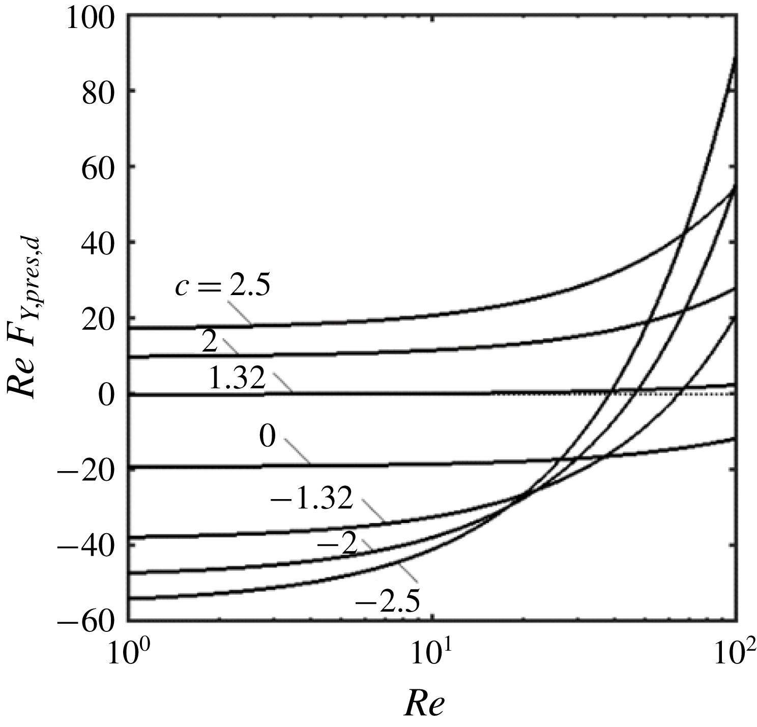
. The forces acting in the
 $y$
-direction are quite sensitive to variations of
 $Re$
, especially for waves propagating upstream, as illustrated in figure 17.
Distributions of
 $Ref_{X,inter}$
(a) and of
 $Ref_{X,visc}$
(b) for
 $Re=1,100$
,
 $A=0.2$
,
 $\unicode[STIX]{x1D6FC}=0.01$
. Solid and dashed lines correspond to
 $Re=1$
and
 $Re=100$
, respectively. Thick and thin lines identify the local and mean values, respectively. The special value of
 $c$
for these conditions is
 $c_{cr,pi}=1.96$
. Results in (b) overlap for
 $c=0$
. Mean values in (b) have been multiplied by 4 for display purposes.

Variations of
 $ReF_{Y,pres,d}$
for
 $A=0.2$
,
 $\unicode[STIX]{x1D6FC}=0.01$
and
 $c=0,\pm 1.32,\pm 2,\pm 2.5$
as a function of
 $Re$
.

7 Mixing induced by the one-wall vibrations
Particles follow straight lines in a smooth channel producing no transverse mixing. Wall corrugations provide spatial modulations, but additional mixing may occur either (i) through dynamical effects, i.e. system bifurcation producing streamwise vortices and/or travelling waves (Floryan Reference Floryan2015; Gepner & Floryan Reference Gepner and Floryan2016) or (ii) through kinematic effects created by the system geometry and resulting in a chaotic advection (Aref Reference Aref1984; Sturman et al. Reference Sturman, Ottino and Wiggins2006). In all cases one is interested in creating transverse motions that will stretch and fold volumes of fluid over the channel cross-section. Such stirring reduces the mixing length by decreasing the average distance over which diffusion must act in the transverse direction to homogenize unmixed volumes. Wall movement represents a different concept as it directly produces mechanical mixing with its effectiveness depending on the type of movement. Wall vibrations are of interest as, if one focusses attention on a specific spatial location, the surface waves may be viewed as a piston moving up and down, assisting diffusion of scalar quantities across the channel. The mixing process is especially effective close to the wall where the axial translation is very slow and the transverse movement is very large. This is a kinematic process driven by a known velocity field and, thus, it does not require any dynamic analysis.
The velocity field exhibits two periodicities, one in space with wavelength
 $\unicode[STIX]{x1D706}=2\unicode[STIX]{x03C0}/\unicode[STIX]{x1D6FC}$
and one in time with period
 $T=2\unicode[STIX]{x03C0}/\unicode[STIX]{x1D6FC}c$
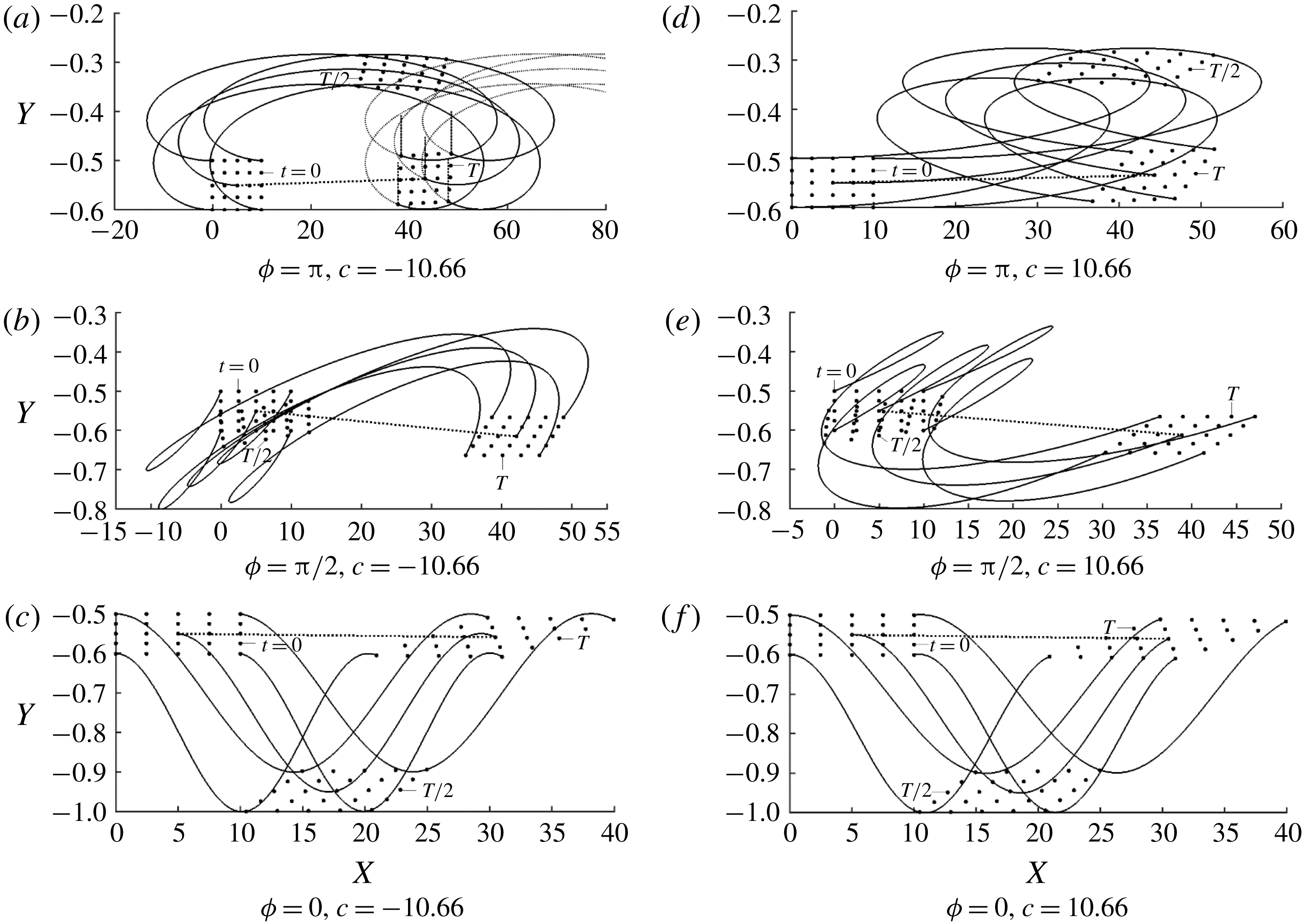
. The particle trajectories exhibit complex structure due to the existence of shear and changes of the
 $X$
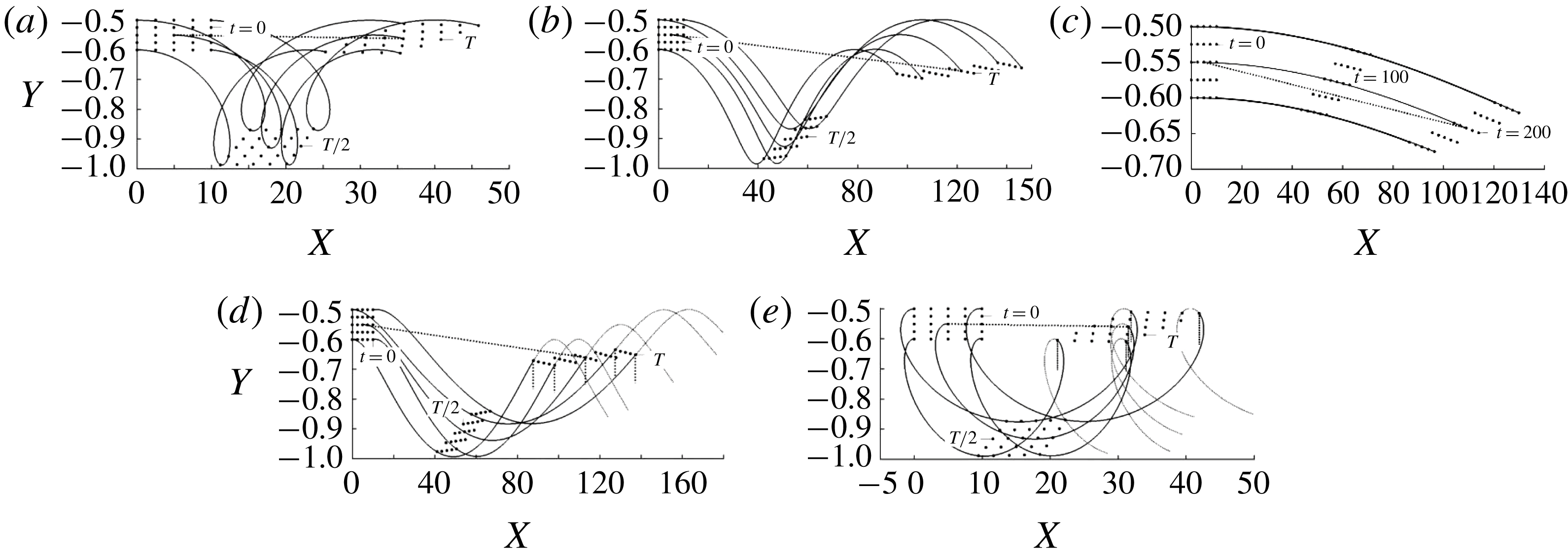
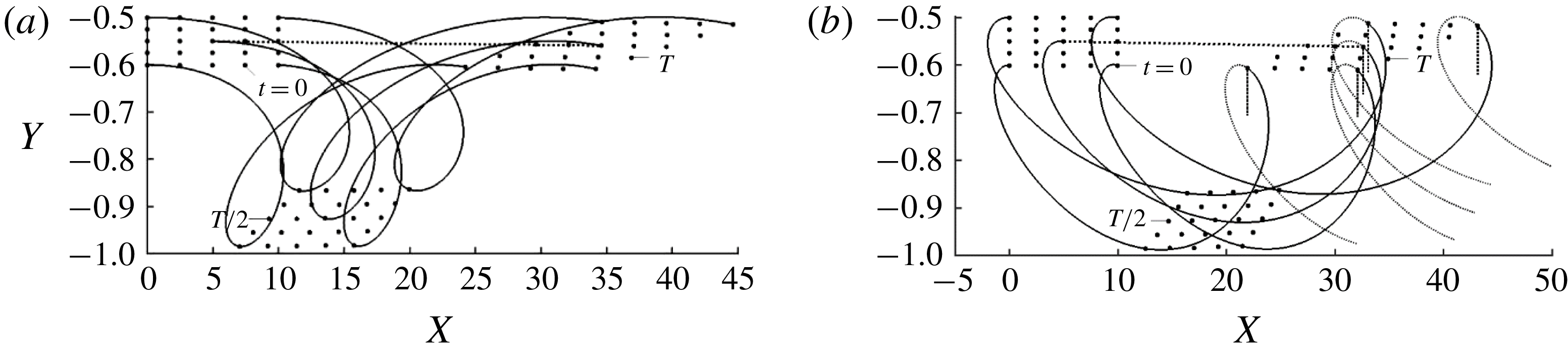
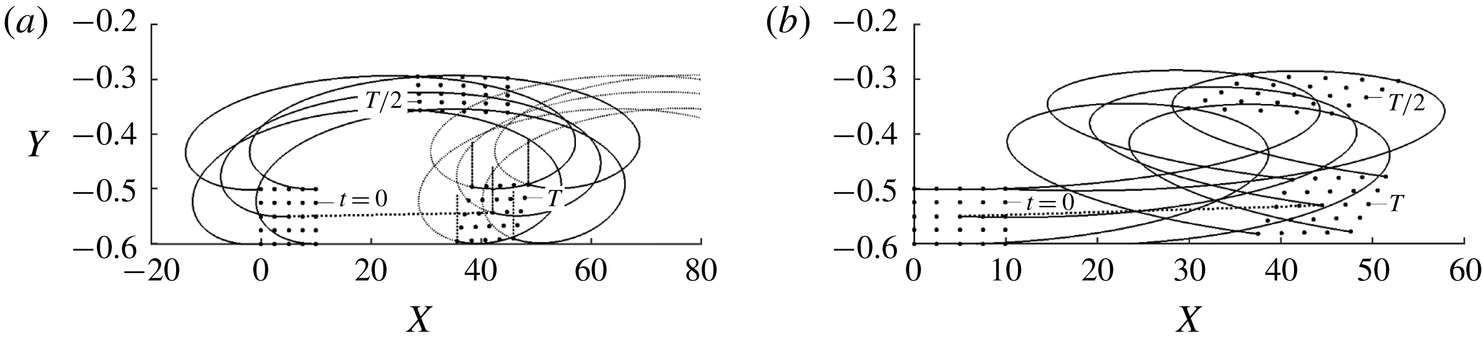
-velocity when a particle moves across the channel. Figure 18 displays trajectories of particle blobs released at the same time and location extending over one period. Their form results from a combination of the axial movement driven by the axial pressure gradient and the transverse movement driven by the waves. The former creates strong shear which leads to blob stretching. The latter changes particle positions in the shear field affecting this stretching. The trajectories show marginal transverse movement for stationary grooves (
 $c=0$
) as illustrated in figure 18(c). Since in this case the period is undefined, this plot extends over an
 $X$
-distance like that used in the other plots. Slow forward moving waves create a significant transverse movement which, when combined with the axial translation, creates trajectories steep in the upward portion and gentle in the downward portion (see results for
 $c=2.66$
in figure 18
d). Waves fast enough to cause flow separation initiate the same transverse movement but occurring over a significantly shorter axial distance. These trajectories acquire a characteristic backward looping, as illustrated in figure 18(e) for
 $c=10.66$
. The steepness of their upper portions, as compared to their lower portions, is more pronounced. Slow backward moving waves create trajectories with opposite characteristics, i.e. they are steep in the lower portions and rather smooth in the upper portions (see results for
 $c=-2.66$
in figure 18
b). Increase of their speed to
 $c=-10.66$
produces trajectories very smooth in the upper portions and but very steep and back looping close to the vibrating wall.
Trajectories of rectangular blobs of size (10
 $\times$
0.1) made of
 $5\times 5$
particles with their top left corners placed initially at
 $(X,Y)=(0,-0.5)$
for
 $Re=1$
,
 $A=0.2$
,
 $\unicode[STIX]{x1D6FC}=0.01$
, and
 $c=-10.66,-2.66,0,2.66,10.66$
in (a–e), respectively, at times
 $t=T/2$
,
 $t=T$
where
 $T=2\unicode[STIX]{x03C0}/\unicode[STIX]{x1D6FC}c$
is the period of the oscillations. Thin solid lines identify trajectories of the central and corner particles, dotted lines connect positions of the central particles at the beginning and end of the cycle. Short vertical dotted lines in (d,e) identify the end of the cycle.

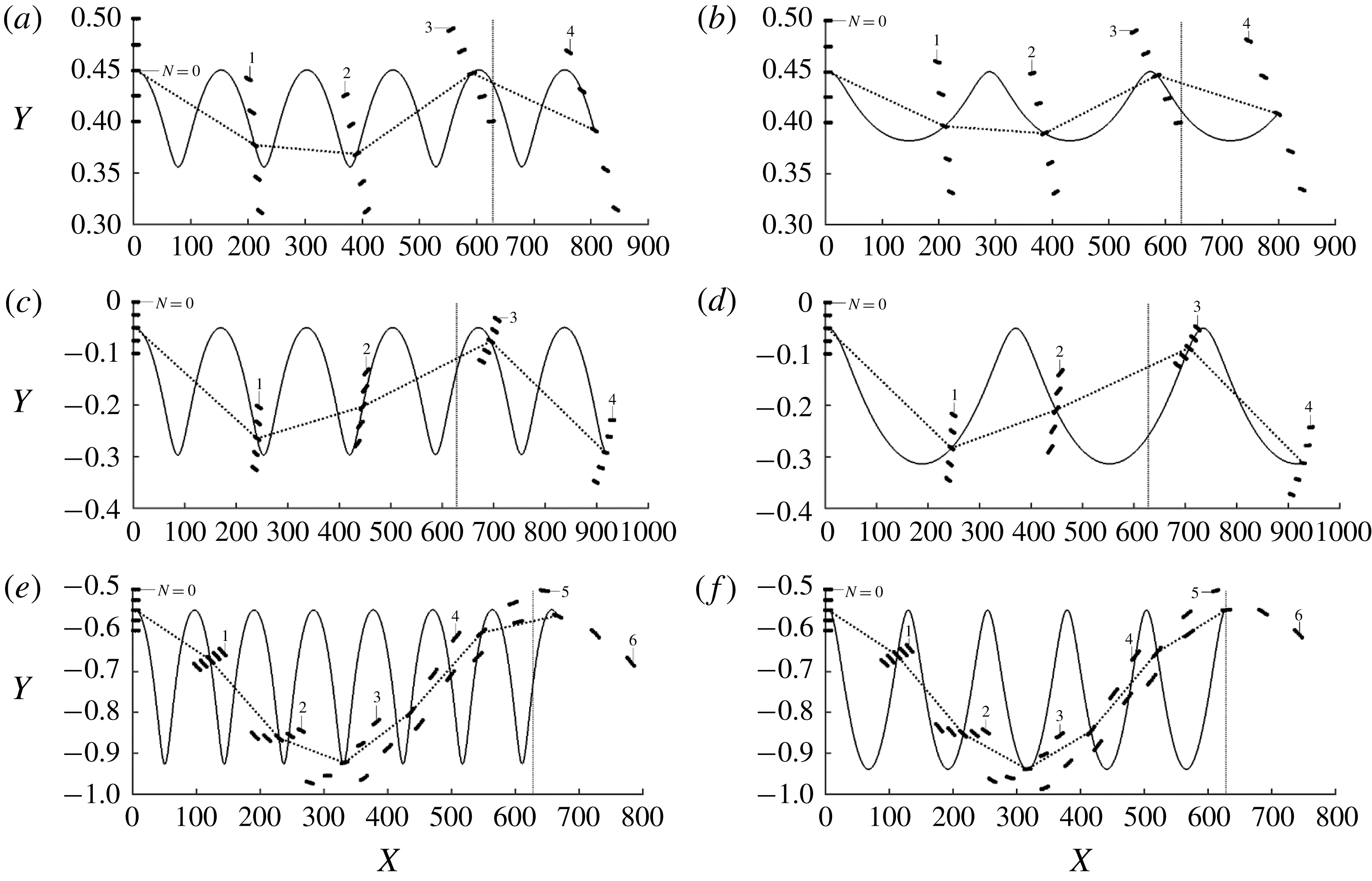
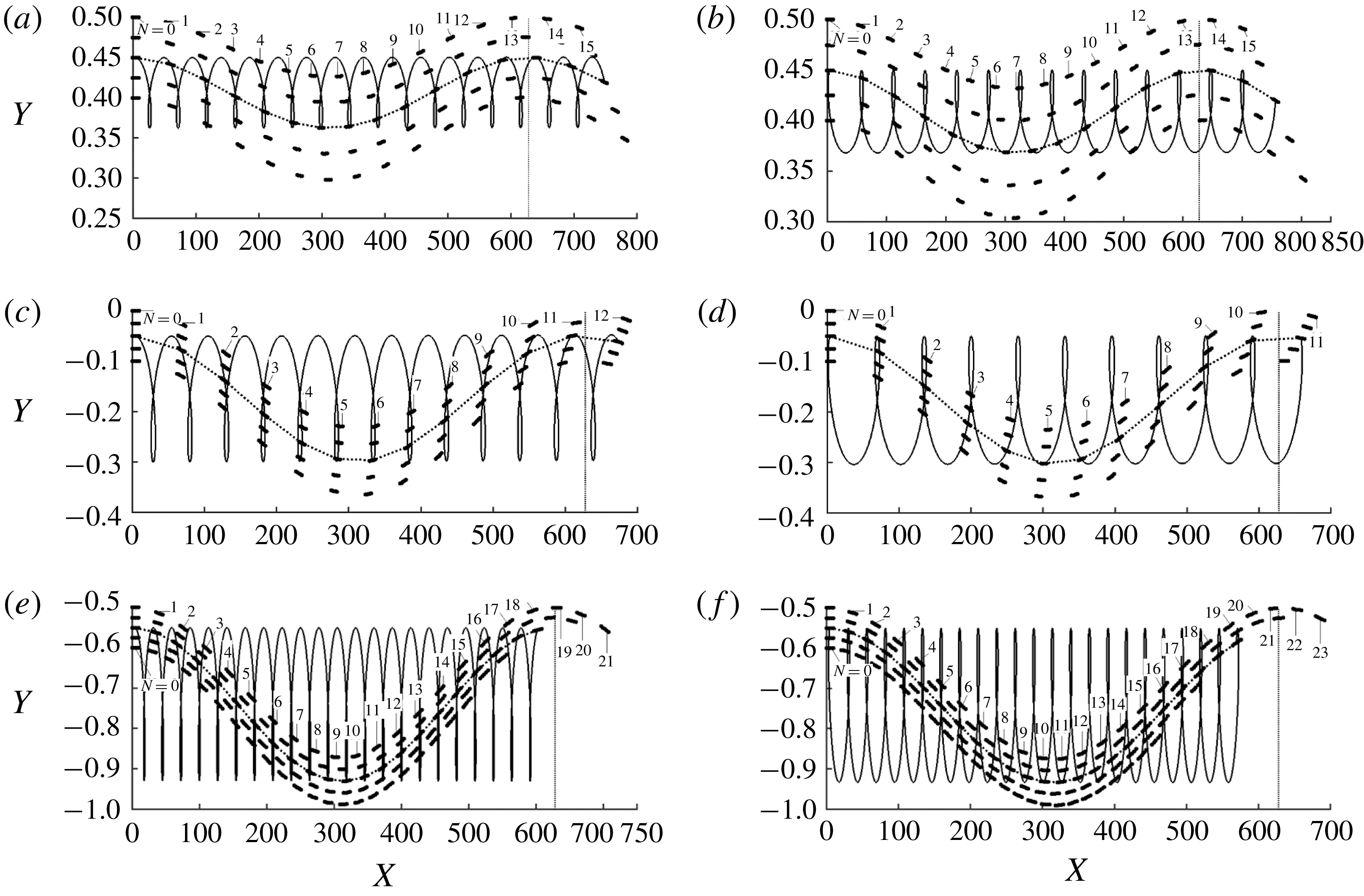
Interesting features of mixing are revealed by following blobs over an
 $X$
-distance corresponding approximately to a single wavelength, as illustrated in figure 19 for slow waves and figure 20 for faster waves. These blobs were released at different distances from the wall, resulting in different magnitudes of the axial velocity component. It can be seen that the amplitude of the transverse movement decreases with distance away from the wall (compare figures 19
a,b with e,f, and 20
a,b with e,f). The peak-to-peak
 $X$
-distance on a particle trajectory is different from the
 $X$
-distance covered by a particle during one wave cycle; it is shorter for waves propagating upstream and longer for waves propagating downstream. This leads to a long-wavelength
 $X$
-periodicity of the blob movement clearly visible in figure 20 and corresponding approximately to the wave wavelength. It takes many more wave cycles to traverse this distance when the blob is released close to the wall compared to the situation when the blob is released close to the channel centre (compare figures 19
c,d with e,f, and 20
c,d with e,f). The mean axial velocity is much smaller in the former case compared to the latter case. One may also observe that many more wave cycles are required for waves with large phase speeds when compared with waves with small phase speeds (compare figures 19 and 20). The forward moving waves accelerate the blob while the backward moving waves decelerate it. This effect is clearly visible in the case of slow waves (see figure 19) but becomes overshadowed by the complexity of trajectories for fast waves (figure 20).
Blobs undergo shearing deformation whose magnitude is related to their mean position in the shear layer. Relatively little deformation is observed for blobs released near the channel centre but they move quite fast and cover the axial distance equal to one wavelength using 3–4 cycles for the slow waves (see figure 19 c,d) and 10 cycles for the fast waves (see figure 20 c,d). Large deformations are observed for blobs released near the vibrating wall but such blobs move slowly; this effect is clearly visible in the case of fast waves where 23 cycles are required to cover the same distance (see figure 20 e,f). The effectiveness of shearing per length of the channel is therefore different from the same effectiveness measured per unit time. The former one is likely of more interest in applications and this is why figures 19 and 20 use spatial representation.
The effects of
 $Re$
are illustrated in figure 21. The trajectories remain qualitatively the same regardless of
 $Re$
, with their segments close to the wall bending in the direction of the wave motion resulting in the obliqueness of the back loops.
Trajectories of blobs of size (
 $10\times 0.1$
) made of
 $5\times 5$
particles with their top left corners placed initially at
 $(X,Y)=(0,0.5),(0,0),(0,-0.5)$
in (a–f), respectively, at times equal to
 $t=N\ast T$
where
 $T=2\unicode[STIX]{x03C0}/\unicode[STIX]{x1D6FC}c$
is the period of the oscillations. Thin solid lines identify trajectories of the central particles, dotted lines connect positions of these particles at times
 $t=N\ast T$
. (a,c,e) Show
 $c=-2.66$
and (b,d,f)
 $c=2.66$
. All other conditions are as in figure 18. The vertical line in each panel identifies the end of the wave wavelength.


Trajectories of blobs for
 $Re=100$
, and
 $c=-10.66$
and
 $c=10.66$
in (a,b), respectively. All remaining conditions are the same as in figure 18. Short vertical dotted lines in (b) identify the end of the cycle.

A quantitative measure of mixing is provided by the length
 $L$
of trajectories of particles travelling over one wavelength in the
 $X$
-direction. The length in the smooth channel for conditions used in table 1 is
 $\unicode[STIX]{x1D706}=2\unicode[STIX]{x03C0}/\unicode[STIX]{x1D6FC}=628.3$
and serves as the reference. Data displayed in this table demonstrate that trajectories are practically unaffected by the introduction of corrugations. Vibrations however produce significant changes which increase with
 $|c|$
, regardless of the direction of wave propagation. The downstream travelling waves are more effective when
 $Re=1$
and the lengths of their trajectories remain unaffected by an increase of the Reynolds number to
 $Re=100$
. The upstream-propagating waves are strongly affected by
 $Re$
with trajectory lengths increasing by approximately 80 % when
 $Re$
increases from
 $Re=1$
to
 $Re=100$
. Such waves appear to be significantly more effective at higher
 $Re$
than the downstream travelling waves. Such waves are also more energy efficient, as discussed in § 5.
Lengths
 $L/\unicode[STIX]{x1D706}$
of trajectories of particles released at
 $(X,Y)=(0,-0.5)$
for
 $A=0.2$
,
 $\unicode[STIX]{x1D6FC}=0.01$
travelling over one wavelength
 $\unicode[STIX]{x1D706}=2\unicode[STIX]{x03C0}/\unicode[STIX]{x1D6FC}$
in the
 $X$
-direction.

8 Vibrations of both walls
We shall investigate how vibrations of the second wall affect the system response and what the effect is of a phase difference between the upper and lower waves. We shall refer to variations of the relative position of these waves as wave tuning/de-tuning. The channel geometry is described by (2.2) and the Galileo transformation leads to the following geometry description
 $$\begin{eqnarray}\displaystyle y_{U}(x)=1+A_{U}\cos (\unicode[STIX]{x1D6FC}x),\quad y_{L}(x)=-1+A_{L}\cos (\unicode[STIX]{x1D6FC}x+\unicode[STIX]{x1D719}). & & \displaystyle\end{eqnarray}$$
This problem can be viewed as a pattern interaction problem with
 $\unicode[STIX]{x1D719}$
defining the relative position of both wave patterns and serving as a de-tuning parameter. The solution was determined using a method analogous to that described in § 3 but details are not given due to their length. Results displayed in figure 22 demonstrate that the phase angle
 $\unicode[STIX]{x1D719}$
has a very strong effect, with the waves effectively unable to affect the pressure gradient for perfect tuning (
 $\unicode[STIX]{x1D719}=0$
), i.e. the waves are in phase, and have a very strong effect for perfect de-tuning (
 $\unicode[STIX]{x1D719}=\unicode[STIX]{x03C0}$
), i.e. the waves are out of phase. The former situation corresponds to a channel in the form of a periodic wave train while the latter corresponds to a channel with a system of expansion/contraction waves. The drag reducing abilities remain marginally affected as
 $\unicode[STIX]{x1D719}$
decreases from
 $\unicode[STIX]{x1D719}=\unicode[STIX]{x03C0}$
to
 $\unicode[STIX]{x1D719}\approx 0.5\unicode[STIX]{x03C0}$
, but further reduction rapidly reduces
 $B$
(see figure 22). The effectiveness of a system involving vibrations of both walls with perfect de-tuning
 $(\unicode[STIX]{x1D719}=\unicode[STIX]{x03C0})$
is illustrated in figure 23. Comparison with the results for a single vibrating wall (figure 10) shows an order of magnitude increase of the pressure gradient correction.
Variations of the pressure gradient correction
 $ReB$
as a function of
 $c$
and
 $\unicode[STIX]{x1D719}$
for a channel with two vibrating walls. The channel geometry is described by (8.1) with
 $A=A_{L}=A_{U}=0.2$
. The light shaded area identifies conditions leading to a reduction of the pressure gradient while the dark shaded area identifies conditions where the pressure gradient must change direction to maintain the same flow rate.

Variations of the pressure gradient correction
 $ReB$
as a function of
 $c$
and
 $A=A_{L}=A_{U}$
for a channel with two walls vibrating out of phase. The channel geometry is described by (8.1) with
 $\unicode[STIX]{x1D719}=\unicode[STIX]{x03C0}$
. The light shaded area identifies conditions leading to reduction of the pressure gradient while the dark shaded area identifies conditions where the pressure gradient must change direction to maintain the same flow rate.

The energy efficiency of the system changes significantly through the addition of the second wall vibrations. Distribution of
 $Re\unicode[STIX]{x0394}{\wp}_{net}$
as a function of
 $c$
and
 $\unicode[STIX]{x1D719}$
illustrated in figure 24 demonstrates the existence of a range of the downstream propagating waves which lead to the overall reduction of the energy consumption with some of these waves leading to the reduction of pressure losses (compare figures 22 and 24). This range changes marginally as a function of the phase difference
 $\unicode[STIX]{x1D719}$
but the energy efficiency changes significantly in favour of the perfectly de-tuned waves
 $(\unicode[STIX]{x1D719}=\unicode[STIX]{x03C0})$
. The range of phase speeds which leads to the lowering of the energy consumption is very wide for waves with small amplitudes, where the effect is weak, but narrow for large amplitudes where the effect is strong (see figure 25). A large part of this range overlaps with conditions leading to the reduction of pressure gradient, as demonstrated by comparisons of figures 23 and 25.
Variations of the energy savings
 $Re\unicode[STIX]{x0394}{\wp}_{net}$
as a function of
 $c$
and
 $\unicode[STIX]{x1D719}$
for a channel with two vibrating walls. The channel geometry is described by (8.1) with
 $A=A_{L}=A_{U}=0.2$
. Shaded area identifies conditions leading to the reduction of power consumption below the smooth channel level.

Variations of the energy savings
 $Re\unicode[STIX]{x0394}{\wp}_{net}$
as a function of
 $c$
and
 $A=A_{L}=A_{U}$
for a channel with two walls vibrating out of phase. The channel geometry is described by (8.1) with
 $\unicode[STIX]{x1D719}=\unicode[STIX]{x03C0}$
. Shaded area identifies conditions leading to the reduction of power consumption below the smooth channel level.

Vibrations affect velocity distributions as illustrated in figure 26. The character of the flow changes is more pronounced than those observed for the one-wall vibrations illustrated in figure 15. In the case of the forward moving waves (figure 26 a), it is possible to select a wave speed which brings the fluid to a standstill in the wave crest area. The same flow feature should occur in the case of turbulent flow which means that the flow laminarization should occur in the crest areas while the locally turbulent flow should persist in the trough areas. The wall friction will be near zero in the former areas but will increase in the latter areas. Nakanishi et al. (Reference Nakanishi, Mamori and Fukagata2012) demonstrated using numerical experiments that the reduction of pressure gradient can be achieved in such cases. The situation is reversed in the case of the upstream travelling waves with the reduction of velocity occurring in the trough areas and increase in the crest areas (figure 26 b).
Distributions of
 $u$
across the channel for
 $Re=100$
,
 $A=A_{L}=A_{U}=0.2$
and
 $\unicode[STIX]{x1D6FC}=0.01$
with
 $\unicode[STIX]{x1D719}=\unicode[STIX]{x03C0}$
. (a) Displays data for the stationary grooves
 $c=0$
(dotted line) and waves propagating downstream with
 $c=2.66$
(solid line),
 $6.66$
(dashed-dotted line) and
 $10.66$
(dashed line). (b) Displays data for waves propagating upstream with
 $c=-2.66$
(solid line),
 $-6.66$
(dashed-dotted line) and
 $-10.66$
(dashed line); data for
 $c=0$
is added for reference.

Vibrations of both walls generate significant changes to the particle trajectories which result from a combination of the pressure-driven and upper and lower vibrations’ effects. Figure 27 displays trajectories generated by waves with perfect de-tuning (
 $\unicode[STIX]{x1D719}=\unicode[STIX]{x03C0}$
), tuning corresponding to
 $\unicode[STIX]{x1D719}=\unicode[STIX]{x03C0}/2$
and perfect tuning (
 $\unicode[STIX]{x1D719}=0$
). Trajectories produced by the perfectly de-tuned downstream moving waves (figure 27
d) exhibit large back loops with the largest shear deformation occurring half-way through the cycle with the blob recovering during the next half-cycle. The back loops are significantly reduced for the upstream moving waves (figure 27
a) with minimal shear deformation between the beginning and the end of the cycle. In both cases, the particles lift above the release point, the amplitude of the
 $Y$
-movement is limited to approximately 0.3 and the
 $X$
-distance travelled is approximately 50. Change of tuning to
 $\unicode[STIX]{x1D719}=\unicode[STIX]{x03C0}/2$
produces complex trajectories. In the case of the downstream moving waves, the particles move above the release point during the first half of the cycle and follow a back-looping movement returning to the starting position and move below the release point during the next half of the cycle and rapidly translate forward (figure 27
e). The structure of the movement is similar for the upstream moving waves with the particles moving below the release point and back looping during the first half of the cycle and moving above the release point and rapidly translating forward during the second half of the cycle (see figure 27
b). The back looping is significantly reduced as compared to
 $\unicode[STIX]{x1D719}=\unicode[STIX]{x03C0}$
, the amplitude of the
 $Y$
-variations increases to approximately 0.4 and the
 $X$
-distance travelled is reduced to approximately 40. Perfect tuning results in the elimination of the back loops, further increase of the
 $Y$
-amplitude to approximately 0.5 and reduction of the
 $X$
-distance to approximately 30 (see figure 27
c,f). The particles move below the release point and return to it at the end of the cycle with trajectories for the upstream and downstream moving waves being nearly identical. It may be concluded that the perfect de-tuning promotes the
 $X$
-movement while reducing the
 $Y$
-translations, while the prefect tuning promotes the
 $Y$
-translation while reducing the
 $X$
-movement.
Positions of rectangular blobs of size (10
 $\times$
0.1) made of
 $5\times 5$
particles with their top left corners placed initially at
 $(X,Y)=(0,-0.5)$
for
 $Re=1$
,
 $A(=A_{L}=A_{U})=0.2$
,
 $\unicode[STIX]{x1D6FC}=0.01$
, at times
 $t=T/2$
and
 $t=T$
, where
 $T=2\unicode[STIX]{x03C0}/\unicode[STIX]{x1D6FC}c$
is the period of the oscillations. Thin solid lines identify trajectories of the central and corner particles, dotted lines connect positions of the central particles at the beginning and end of the cycle. Short vertical dotted lines in (a) identify the end of the cycle.

Another insight is offered by determining the lengths of particle trajectories whose change with respect to the length of similar trajectories in smooth channels can serve as a measure of mixing effectiveness. These lengths illustrated in table 2 demonstrate marginal changes in the perfectly tuned channels but, in the case of the perfectly de-tuned channels, increase by approximately 50 % above trajectories generated by the one-wall vibrations. The upstream-propagating waves are more effective at small
 $Re$
while the direction of propagation plays no role at larger
 $Re$
(see data in table 2 for
 $Re=100$
). An increase of
 $Re$
decreases the effectiveness of the upstream-propagating waves and increases the effectiveness of the downstream-propagating waves. The latter are however preferable as they are significantly more energy efficient, as discussed at the beginning of this section.
Lengths
 $L/\unicode[STIX]{x1D706}$
of trajectories of particles released at
 $(X,Y)=(0,-0.5)$
for
 $A=0.2$
,
 $\unicode[STIX]{x1D6FC}=0.01$
travelling over one wavelength
 $\unicode[STIX]{x1D706}=2\unicode[STIX]{x03C0}/\unicode[STIX]{x1D6FC}$
in the
 $X$
-direction for perfectly tuned vibrations (
 $\unicode[STIX]{x1D719}=0$
) and perfectly de-tuned vibrations (
 $\unicode[STIX]{x1D719}=\unicode[STIX]{x03C0}$
).

The evolution of blobs over an
 $X$
-distance corresponding approximately to a single wavelength
 $\unicode[STIX]{x1D706}$
is illustrated in figure 28. The increase of tuning, from the perfect one (
 $\unicode[STIX]{x1D719}=0$
) illustrated in figure 28(c,f) to the perfect de-tuning (
 $\unicode[STIX]{x1D719}=\unicode[STIX]{x03C0}$
) illustrated in figure 28(a,d), decreases the axial travel time from approximately 21 cycles in the former case to approximately 12 cycles in the latter case. The blob shear deformation in the
 $X$
-direction is largest for the perfectly tuned waves but in the
 $Y$
-direction it is largest for the waves with the intermediate tuning corresponding to
 $\unicode[STIX]{x1D719}=\unicode[STIX]{x03C0}/2$
. In this case, the blob particles form nearly a single line (see figure 28
e).
Positions of the blobs from figure 27 at times equal to
 $t=N\ast T$
for
 $c=-10.66$
, 10.66 in (a–c) and (d–f), respectively. Thin solid lines identify trajectories of central particles; dotted lines connect positions of these particles at times
 $t=N\ast T$
. All other conditions are as in figure 27. The vertical line in each panel identifies the end of the wave wavelength.

The effects of
 $Re$
are illustrated in figure 29. The trajectories remain qualitatively the same for
 $Re=1$
and 100 (compare figures 28 and 29) without any bending found in the case of the single-wall vibrations but with an increase of shear deformation.
Trajectories of blobs for
 $Re=100$
, perfect de-tuning
 $\unicode[STIX]{x1D719}=\unicode[STIX]{x03C0}$
and phase speeds
 $c=-10.66$
, 10.66 in (a,b), respectively. The remaining conditions are the same as in figure 27. Short vertical dotted lines in (a) identify the end of the cycle.

9 Conclusions
Pressure losses and mixing in vibrating channels were analysed. The analysis was focused on vibrations in the form of long-wavelength waves travelling either downstream or upstream. The effects of de-tuning between the upper and lower waves were considered, with in-phase waves (perfect tuning) resulting in a channel in the form of a periodic wave train and out-of-phase waves (perfect de-tuning) resulting in a channel modified by a system of expansion/contraction waves.
The wave-induced changes in the velocity field were described. It was shown that fast enough waves produce flow separation, with forward moving waves producing separation at the wave crest and backward moving waves producing separation at the wave trough.
The analysis of the forces opposing the fluid movement was carried out by comparing the pressure gradient required to drive a specified flow rate through a vibrating channel with the pressure gradient required to drive the same fluid volume through a stationary channel. It was shown that forward moving waves can reduce pressure losses, with larger reduction found for faster waves. The mechanisms responsible for this effect were identified. The presence of waves results in an interaction between the pressure field and the wall geometry. The resulting axial pressure force may either assist or oppose the fluid movement, depending on the phase difference between the wave pattern and the pattern of the periodic part of the pressure field. The conditions leading to the phase shift, changing the direction of the pressure force from opposing the fluid motion to supporting this motion, were determined. The fluid motion is also affected by the friction which, in general, opposes the fluid movement. It was shown that fast forward moving waves, which create large separation zones, lead to a change in direction of the friction force when averaged over one wavelength, with this force assisting the fluid movement. Use of the perfectly de-tuned waves on both walls increases the pressure gradient reducing effect by an order of magnitude when compared with single-wall vibrations, while perfect tuning changes this effect marginally. Conditions when the externally imposed pressure gradient must be reversed to prevent fluid acceleration have been identified. No externally imposed pressure gradient is required at the reversal point as the desired flow rate is driven by vibrations only. This demonstrates the potential of surface vibrations for generating a propulsive force. Analysis of energy fluxes demonstrates that it is possible to identify waves which reduce the overall energy consumption despite of energy expenditures associated with their actuation. Use of the two-wall vibrations is required in this case, with the perfectly de-tuned waves being more effective.
An analysis of particle trajectories was carried out to determine the vibrations’ potential for improvement of transverse mixing. The velocity field exhibits periodicity in time as well as periodicity in the axial direction, and varies parabolically in the transverse direction. As a result, particle trajectories exhibit two periodicities, one temporal and one spatial, with their axial movements mediated by altering position in the shear field. They move rapidly in the axial direction when placed near the channel centre, where the axial velocity component is dominant. They move slowly when placed near the channel wall, where the transverse velocity component is dominant. Significant transverse movement occurs within one time period, including back loops, with the particles travelling across the channel by a distance equal to nearly 50 % of the channel height. This distance strongly depends upon particle position with respect to the vibrating wall, with particles near the wall exhibiting a larger range of movements. The particles travel over the same transverse distance when moving in the axial direction over a distance approximately equal to the wave wavelength, resulting in a near double periodicity of trajectories. Out-of-phase vibrations of both walls (perfect de-tuning) produce large changes in the pressure gradient while, at the same time, they increase lengths of particle trajectories generating larger mixing potential. In-phase vibrations of both walls (perfect tuning) reduce the lengths of particle trajectories and, thus, reduce potential for mixing while producing changes in the pressure gradient like those generated by one wall vibrations. Use of the perfectly de-tuned waves is recommended due to their better energy efficiency as well as higher mixing potential.
Acknowledgements
This work has been carried out with support from the Natural Sciences and Engineering Research Council (NSERC) of Canada.
Appendix A. Definitions of functions used in § 3
 $$\begin{eqnarray}\displaystyle G_{1}=2-A\cos (\unicode[STIX]{x1D709}),\quad G_{2}=4+\unicode[STIX]{x1D6FC}^{2}A^{2}\sin ^{2}(\unicode[STIX]{x1D709})(\unicode[STIX]{x1D702}-1)^{2},\quad G_{3}=\unicode[STIX]{x1D702}_{x}^{2}+\unicode[STIX]{x1D702}_{y}^{2}\qquad & & \displaystyle\end{eqnarray}$$
 $$\begin{eqnarray}\displaystyle F_{1}=\unicode[STIX]{x1D702}_{xx}G_{3}^{-1}={\textstyle \frac{1}{4}}\unicode[STIX]{x1D6FC}^{2}[-G_{1}A\cos (\unicode[STIX]{x1D709})+2A^{2}\sin ^{2}(\unicode[STIX]{x1D709})](\unicode[STIX]{x1D702}-1)+O(\unicode[STIX]{x1D6FC}^{4}), & & \displaystyle\end{eqnarray}$$
 $$\begin{eqnarray}\displaystyle F_{2}=Re\unicode[STIX]{x1D702}_{x}G_{3}^{-1}=-{\textstyle \frac{1}{4}}\unicode[STIX]{x1D6FC}ReG_{1}A\sin (\unicode[STIX]{x1D709})(\unicode[STIX]{x1D702}-1)+O(\unicode[STIX]{x1D6FC}^{3}), & & \displaystyle\end{eqnarray}$$
 $$\begin{eqnarray}\displaystyle F_{3}=Re\unicode[STIX]{x1D702}_{y}G_{3}^{-1}={\textstyle \frac{1}{2}}ReG_{1}-{\textstyle \frac{1}{8}}ReG_{1}(G_{2}-4)+O(\unicode[STIX]{x1D6FC}^{4}), & & \displaystyle\end{eqnarray}$$
 $$\begin{eqnarray}\displaystyle F_{4}=2\unicode[STIX]{x1D6FC}\unicode[STIX]{x1D702}_{x}G_{3}^{-1}=-{\textstyle \frac{1}{2}}\unicode[STIX]{x1D6FC}^{2}G_{1}A\sin (\unicode[STIX]{x1D709})(\unicode[STIX]{x1D702}-1)+O(\unicode[STIX]{x1D6FC}^{4}), & & \displaystyle\end{eqnarray}$$
 $$\begin{eqnarray}\displaystyle F_{5}=\unicode[STIX]{x1D6FC}^{2}G_{3}^{-1}={\textstyle \frac{1}{4}}{\unicode[STIX]{x1D6FC}^{2}G}_{1}^{2}+O(\unicode[STIX]{x1D6FC}^{4}),\quad F_{6}=\unicode[STIX]{x1D6FC}ReG_{3}^{-1}={\textstyle \frac{1}{4}}\unicode[STIX]{x1D6FC}ReG_{1}^{2}+O(\unicode[STIX]{x1D6FC}^{3}), & & \displaystyle\end{eqnarray}$$
 $$\begin{eqnarray}\displaystyle F_{7}=\unicode[STIX]{x1D702}_{x}=-\unicode[STIX]{x1D6FC}A(\unicode[STIX]{x1D702}-1)\sin (\unicode[STIX]{x1D709})G_{1}^{-1},\quad F_{8}=\unicode[STIX]{x1D702}_{y}=2G_{1}^{-1}, & & \displaystyle\end{eqnarray}$$
 $$\begin{eqnarray}\displaystyle \left.\begin{array}{@{}c@{}}\displaystyle H_{1}=-{\textstyle \frac{1}{80}}\unicode[STIX]{x1D702}^{6}+{\textstyle \frac{3}{32}}\unicode[STIX]{x1D702}^{4}-{\textstyle \frac{1}{8}}\unicode[STIX]{x1D702}^{3}-{\textstyle \frac{27}{280}}\unicode[STIX]{x1D702}^{2}+{\textstyle \frac{1}{8}}\unicode[STIX]{x1D702}+{\textstyle \frac{17}{1120}},\\ \displaystyle H_{2}=-{\textstyle \frac{1}{80}}\unicode[STIX]{x1D702}^{6}+{\textstyle \frac{1}{4}}\unicode[STIX]{x1D702}^{3}+{\textstyle \frac{9}{560}}\unicode[STIX]{x1D702}^{2}-{\textstyle \frac{1}{4}}\unicode[STIX]{x1D702}-{\textstyle \frac{1}{280}},\end{array}\right\} & & \displaystyle\end{eqnarray}$$
 $$\begin{eqnarray}\displaystyle H_{3}={\textstyle \frac{1}{12}}\unicode[STIX]{x1D702}^{4}-{\textstyle \frac{1}{6}}\unicode[STIX]{x1D702}^{3}-{\textstyle \frac{1}{10}}\unicode[STIX]{x1D702}^{2}+{\textstyle \frac{1}{6}}\unicode[STIX]{x1D702}+{\textstyle \frac{1}{60}},\quad H_{4}=-{\textstyle \frac{1}{12}}\unicode[STIX]{x1D702}^{4}+{\textstyle \frac{1}{10}}\unicode[STIX]{x1D702}^{2}-{\textstyle \frac{1}{60}}, & & \displaystyle\end{eqnarray}$$
 $$\begin{eqnarray}\displaystyle \left.\begin{array}{@{}c@{}}\displaystyle H_{5}={\textstyle \frac{1}{24}}\unicode[STIX]{x1D702}^{6}-{\textstyle \frac{1}{4}}\unicode[STIX]{x1D702}^{4}+{\textstyle \frac{1}{6}}\unicode[STIX]{x1D702}^{3}+{\textstyle \frac{69}{280}}\unicode[STIX]{x1D702}^{2}-{\textstyle \frac{1}{6}}\unicode[STIX]{x1D702}-{\textstyle \frac{4}{105}},\\ \displaystyle H_{6}={\textstyle \frac{1}{60}}\unicode[STIX]{x1D702}^{6}-{\textstyle \frac{1}{3}}\unicode[STIX]{x1D702}^{3}-{\textstyle \frac{3}{140}}\unicode[STIX]{x1D702}^{2}+{\textstyle \frac{1}{3}}\unicode[STIX]{x1D702}+{\textstyle \frac{1}{210}},\end{array}\right\} & & \displaystyle\end{eqnarray}$$
 $$\begin{eqnarray}\displaystyle H_{7}=-{\textstyle \frac{1}{8}}\unicode[STIX]{x1D702}^{4}+{\textstyle \frac{1}{6}}\unicode[STIX]{x1D702}^{3}+{\textstyle \frac{3}{20}}\unicode[STIX]{x1D702}^{2}-{\textstyle \frac{1}{6}}\unicode[STIX]{x1D702}-{\textstyle \frac{1}{40}},\quad H_{8}=-{\textstyle \frac{1}{30}}\unicode[STIX]{x1D702}^{6}+{\textstyle \frac{1}{6}}\unicode[STIX]{x1D702}^{4}-{\textstyle \frac{11}{70}}\unicode[STIX]{x1D702}^{2}+{\textstyle \frac{1}{42}},\qquad \quad & & \displaystyle\end{eqnarray}$$
 $$\begin{eqnarray}\displaystyle H_{9}=-{\textstyle \frac{1}{4}}\unicode[STIX]{x1D702}^{3}+{\textstyle \frac{3}{4}}\unicode[STIX]{x1D702}-{\textstyle \frac{1}{2}},\quad H_{10}={\textstyle \frac{1}{4}}\unicode[STIX]{x1D702}^{3}-{\textstyle \frac{3}{8}}\unicode[STIX]{x1D702}^{2}+{\textstyle \frac{1}{8}},\quad H_{11}={\textstyle \frac{1}{2}}\unicode[STIX]{x1D702}^{3}-{\textstyle \frac{1}{2}}\unicode[STIX]{x1D702}^{2}-{\textstyle \frac{1}{2}}\unicode[STIX]{x1D702}+{\textstyle \frac{1}{2}}. & & \displaystyle \nonumber\\ \displaystyle & & \displaystyle\end{eqnarray}$$