




1. Introduction
Heat transfer enhancement by passive or active control is a critical research topic. For passive control, adding wall roughness to heat transfer surfaces, such as transverse/longitudinal ribs (Liou, Hwang & Chen Reference Liou, Hwang and Chen1993; Murata & Mochizuki Reference Murata and Mochizuki2001) and dimples/protrusions (Mahmood, Sabbagh & Ligrani Reference Mahmood, Sabbagh and Ligrani2001; Hwang et al. Reference Hwang, Dong, Hyun and Cho2008), is a simple and widely used control technique. It is well known that there is a similarity between the momentum and heat transfer because the governing equations for scalar and flow fields are similar, with the exception of the pressure term. When the diffusivities for flow and scalar fields are identical, the ratio of the Stanton number  $S_t$ to the skin friction coefficient
 $C_f$, which is referred to as the Reynolds analogy factor,
 $RA=2S_t/C_f$, is close to unity for a smooth wall-bounded flow. However, the wall roughness generally breaks the similarity between the momentum and heat transfer unfavourably, i.e. augmentation of
 $C_f$ is larger than that of
 $S_t$ for rough surfaces. This phenomenon is supported by many experimental data (Dipprey & Sabersky Reference Dipprey and Sabersky1963; Kays & Crawford Reference Kays and Crawford1993; Bons Reference Bons2002), theoretical analysis (Katoh, Choi & Azuma Reference Katoh, Choi and Azuma2000) and direct numerical simulations (DNS) data (Forooghi, Stripf & Frohnapfel Reference Forooghi, Stripf and Frohnapfel2018; MacDonald, Hutchins & Chung Reference MacDonald, Hutchins and Chung2019; Peeters & Sandham Reference Peeters and Sandham2019; Kuwata Reference Kuwata2021). The key factor that causes an unfavourable breakdown of the Reynolds analogy is an increased pressure drag acting on roughness elements. The pressure drag directly increases
 $C_f$ but not
 $S_t$ because no corresponding mechanisms exists for an increase in the heat transfer rate (Katoh et al. Reference Katoh, Choi and Azuma2000; MacDonald et al. Reference MacDonald, Hutchins and Chung2019; Kuwata Reference Kuwata2021). Therefore, the breakdown of the Reynolds analogy can be circumvented to some degree by the use of the roughness that does not offer the pressure drag – for example, obstacles aligned with the flow directions (Stalio & Nobile Reference Stalio and Nobile2003; Jin & Herwig Reference Jin and Herwig2014; Stroh et al. Reference Stroh, Schäfer, Forooghi and Frohnapfel2020). Recent theoretical studies by Alben (Reference Alben2017) and Motoki, Kawahara & Shimizu (Reference Motoki, Kawahara and Shimizu2018) demonstrated the possibility of an optimized shear flow with a much higher heat transfer rate than skin friction, i.e. enabling the favourable breakdown of the Reynolds analogy. Although the optimized shear flows in those studies were driven by an arbitrary body force, it was demonstrated that a heat transfer rate higher than skin friction can be realized by Coriolis force for shear flows subjected to system rotation (Brethouwer Reference Brethouwer2021) and buoyancy force for mixed convection with unstable stratification (Pirozzoli et al. Reference Pirozzoli, Bernardini, Verzicco and Orlandi2017). Nevertheless, to the best of the author's knowledge, there is no report on the passive control technique with a roughness obstacle that yields significant favourable breakdown of the Reynolds analogy.
In contrast to the passive control, several active control techniques successfully achieve favourable breakdown of the Reynolds analogy. Specifically, travelling-wave-like local blowing/suction from the wall is one of the most outstanding techniques to achieve favourable dissimilar heat transfer enhancement (Hasegawa & Kasagi Reference Hasegawa and Kasagi2011; Yamamoto, Hasegawa & Kasagi Reference Yamamoto, Hasegawa and Kasagi2013; Kaithakkal, Kametani & Hasegawa Reference Kaithakkal, Kametani and Hasegawa2020). Notably, the turbulent structure near the wall with travelling-wave-like local blowing/suction is visually similar to the turbulent structure modulated by the spanwise rollers associated with the Kelvin–Helmholtz (K–H) instability, which we encounter commonly in porous wall turbulence (Breugem, Boersma & Uittenbogaard Reference Breugem, Boersma and Uittenbogaard2006; Suga et al. Reference Suga, Matsumura, Ashitaka, Tominaga and Kaneda2010; Kuwata & Suga Reference Kuwata and Suga2016a, Reference Kuwata and Suga2017). This serves as a motivation to exploit the spanwise rollers for the heat transfer control. The aim of the present DNS study is to open the way for the favourable breakdown of the Reynolds analogy by the spanwise rollers. The high-aspect-ratio longitudinal ribs aligned with the flow directions, which can induce the spanwise rollers associated with the K–H instability, were considered in the study. We performed DNS of turbulent heat transfer over high-aspect-ratio longitudinal ribs with Prandtl number unity, and discussed the possibility of the favourable breakdown of the Reynolds analogy by the spanwise rollers in a passive manner.
2. DNS methodology
Figure 1 illustrates a schematic of a turbulent open-channel flow over rib roughness in which the streamwise-aligned longitudinal ribs were mounted regularly at the bottom wall. The computational box was  $L_x=6.0H$ and
 $L_z=3.3H$, with
 $H$ being the clear channel height. The flow was periodic in the streamwise (
 $x$) and spanwise (
 $z$) directions, and simulations were run at a constant streamwise pressure difference. The friction Reynolds number for the clear flow region (
 $0< y< H$) was fixed at
 $Re_\tau =u_\tau H/\nu =300$, where
 $u_\tau$ is the average friction velocity at the position of the rib crest (
 $y=0$), and
 $\nu$ is the kinematic viscosity. An incompressible fluid was considered, and the fluid Prandtl number
 $Pr$ was assumed to be unity. Constant wall temperature
 $T_w$ was specified at the surfaces of the ribs and bottom wall, whereas slip and adiabatic boundary conditions were imposed for the top boundary face. The heat transfer is driven by volumetric heat generation
 $q_v$. In this set of heat transfer and fluid flow conditions, the time-averaged momentum and heat transport equations in non-dimensional form were similar (Kasagi et al. Reference Kasagi, Hasegawa, Fukagata and Iwamoto2010; Hasegawa & Kasagi Reference Hasegawa and Kasagi2011). Specifically, the normalized heat generation in the energy equation corresponds to the normalized mean pressure gradient in the momentum equation. We considered high-aspect-ratio longitudinal ribs with various distances between the neighbouring ribs. The height and width of the rib were
 $h=0.67H$ and
 $w=0.05h$, respectively, which resulted in aspect ratio
 $h/w=20$. The separation between the ribs was varied:
 $s/h=0.05$, 0.075, 0.2, 0.45 and
 $1.2$. For reference, we additionally performed smooth-wall simulation with the box of
 $6.0\,H(x)\times H(y) \times 3.3\,H(z)$.
Configuration of a turbulent open-channel flow over longitudinal ribs.

For the numerical method, in following earlier works (Suga, Chikasue & Kuwata Reference Suga, Chikasue and Kuwata2017; Kuwata, Tsuda & Suga Reference Kuwata, Tsuda and Suga2020; Nishiyama, Kuwata & Suga Reference Nishiyama, Kuwata and Suga2020; Kuwata Reference Kuwata2021), the three-dimensional 27-velocity multiple-relaxation-time lattice Boltzmann method (LBM) for the flow field was used, whereas the scalar field was simulated by the three-dimensional 19-velocity regularized LBM. The number of grid points was determined as  $1080(x)\times 301(y)\times 600(z)$, which yields
 $\varDelta ^+=1.67$ in all directions, with
 $\varDelta ^+$ being the grid spacing normalized by wall unit
 $\nu /u_\tau$. This resolution is comparable to those used in previous DNS (Kuwata & Suga Reference Kuwata and Suga2016a, Reference Kuwata and Suga2019; Kuwata & Kawaguchi Reference Kuwata and Kawaguchi2019; Kuwata & Nagura Reference Kuwata and Nagura2020; Kuwata et al. Reference Kuwata, Tsuda and Suga2020). To validate the independence of grid resolution and box size, we performed grid and domain size sensitivity tests for the case
 $s/h=0.2$ in which
 $S_t$ is the largest among the simulation cases. A comparison of the results for
 $\varDelta ^+=1.67$ and
 $2.5$ confirmed that the differences in
 $S_t$ and
 $C_f$ were within
 $0.7$ % and
 $1.4$ %, respectively. Regarding the domain size, we performed DNS with a domain size enlarged by a factor 1.5 in wall-parallel directions, and found that the difference in the maximum peak values of the Reynolds stresses and turbulent heat fluxes was
 $1.4$ % at most. We also confirmed that the enlargement of the domain size yielded a change of less than
 $0.7$ % in
 $S_t$ and
 $C_f$.
To discuss the profiles of the turbulence statistics near rib roughness from a macroscopic perspective, we considered a variable averaged over the  $x$–
 $z$ plane and time in the following discussion. Superficial and intrinsic averaging operators for a variable
 $\phi (x,y,z)$ are introduced as
 \begin{align}
{\langle \phi \rangle}(y,t)
= \frac{1}{A} \int_x \int_z \phi(x,y,z,t) \,{\rm d}x\,{\rm
d}z, \quad {\langle \phi \rangle}^{f}(y,t) = \frac{1}{A_f}
\int_x \int_z \phi(x,y,z,t) \,{\rm d}x\,{\rm d}z,
\end{align}
where  $A=L_xL_z$ is the area of the
 $x$–
 $z$ plane, and
 $A_{f}$ is the area occupied by the fluid in the
 $x$–
 $z$ plane. Therefore, a relationship exists between the superficial and intrinsic plane-averaged values as
 ${\langle \phi \rangle } =\varphi {\langle \phi \rangle }^{f}$, with the volume fraction of the fluid phase,
 $\varphi =s/(s+w)$, below the roughness crest (
 $y<0$), while
 $\varphi =1$ in the clear flow region (
 $y>0$) for the geometry presented herein. The deviation from the intrinsic averaged value
 $\tilde {\phi }(x,y,z,t)$, which is referred to as the dispersion, is
 \begin{equation} \tilde{\phi}(x,y,z,t) = \phi(x,y,z,t) - {\langle \phi \rangle}^{f}(y,t). \end{equation}
We additionally considered the Reynolds decomposition that decomposes a variable into a time-averaged value  $\bar {\phi }(x,y,z)$ and its fluctuation
 $\phi '(x,y,z,t)$ as
 $\phi (x,y,z,t) = \bar {\phi }(x,y,z)$
 $+\,\phi '(x,y,z,t)$. After a flow had reached a fully developed state, statistical properties were assembled over a period
 $50H/u_\tau$.
All the quantities in plus units  $(\cdot )^+$ are scaled with the average friction velocity
 $u_\tau$ or average friction temperature
 $\theta _\tau$. The friction velocity
 $u_\tau$ was based on the average wall shear stress at the rib crest position,
 $\tau _w=\rho u_\tau ^2$, with
 $\rho$ denoting the fluid density. The average wall shear stress was calculated using the pressure gradient via the momentum balance in the clear flow region as in Kuwata & Suga (Reference Kuwata and Suga2016a, Reference Kuwata and Suga2017):
 \begin{equation} \tau_w A = \int_0^{L_z} \int_0^H \int_0^{L_x} \left( -\frac{\partial \bar{p}}{\partial x} \right) \,{\rm d}x\,{\rm d}y\,{\rm d}z, \end{equation}
where  $A=L_xL_z$ is the
 $x$–
 $z$ plane area. Analogous to the friction velocity, the friction temperature
 $\theta _\tau$ was based on the average wall heat flux evaluated at the rib crest position
 $q_w=\rho c u_\tau \theta _\tau$, with
 $c$ denoting the specific heat. The average wall heat flux was calculated by a heat source for volumetric heating,
 $q_v$, via the energy balance in the clear flow region,
 \begin{equation} q_w A= \int_0^{L_z} \int_0^H \int_0^{L_x} q_v \,{\rm d}x\,{\rm d}y\,{\rm d}z, \end{equation}
where the volumetric heat source  $q_v$ has a non-zero constant value in the fluid phase but value zero in the solid phase.
3. Results and discussion
To discuss briefly augmentations of heat and momentum transfer by the rib roughness, we investigate the skin friction coefficient  $C_f$ and Stanton number
 $S_t$, which are given as
 $C_f=2/(U_b^+)^2$ and
 $S_t=1/(U_b^+\varTheta _a^+)$, respectively. Here,
 $U_b$ and
 $\varTheta _a$ are the bulk mean velocity and arithmetic mean temperature in the clear flow region
 $(y>0)$, which are defined as
 \begin{equation} U_b = \frac{1}{H} \int_0^H {\langle \bar{u} \rangle}\,{{\rm d} y}, \quad \varTheta_a = \frac{1}{H} \int_0^H {\langle \bar{\theta} \rangle}\,{{\rm d} y}, \end{equation}
Note that for the present definition, the identical inner-scaled mean velocity and temperature profiles give  $C_f=2S_t$. Augmentations of
 $S_{t}$ and
 $C_f$ from the corresponding smooth wall values
 $S_{t0}$ and
 $C_{f0}$ are displayed in figure 2(a) along with the DNS data for random cone roughness (Forooghi et al. Reference Forooghi, Stripf and Frohnapfel2018), three-dimensional irregular rough surfaces (Kuwata Reference Kuwata2021), two-dimensional transverse bar roughness (Nagano, Hattori & Houra Reference Nagano, Hattori and Houra2004), porous walls (Nishiyama et al. Reference Nishiyama, Kuwata and Suga2020), and experimental data for turbine roughness (Bons Reference Bons2002). Additionally, figure 2(b) displays the Reynolds analogy factor
 $RA=2S_t/C_f$, which quantifies the similarity between the heat and momentum transfer. For the present definition, the
 $RA$ value is exactly unity when the Reynolds analogy holds because the identical inner-scaled mean velocity and temperature profiles give
 $C_f=2S_t$.
(a) Stanton number  $S_t/S_{t0}$ against the skin friction coefficient
 $C_f/C_{f0}$, and (b) Reynolds analogy factor
 $RA$ against the rib separation
 $s/h$. The DNS data for random cone roughness (Forooghi et al. Reference Forooghi, Stripf and Frohnapfel2018), three-dimensional irregular rough surfaces (Kuwata Reference Kuwata2021), two-dimensional transverse bar roughness (Nagano et al. Reference Nagano, Hattori and Houra2004) and porous walls (Nishiyama et al. Reference Nishiyama, Kuwata and Suga2020), and experimental data for turbine roughness (Bons Reference Bons2002), are included. The thin line in (a) indicates
 $S_t/S_{t0} = C_f/C_{f0}$, and that in (b) indicates
 $RA=1.007$ for a smooth wall.

In figure 2(a), all the reference data are below a line  $S_t/S_{t0} = C_f/C_{f0}$, which is an expected result that indicates the unfavourable breakdown of the Reynolds analogy by the passive controls. By contrast, the present results are all above the line
 $S_t/S_{t0} = C_f/C_{f0}$, which indicate that the augmentation of
 $S_t$ from the smooth wall value is larger than that of
 $C_f$. This favourable breakdown of the Reynolds analogy is quantified by the
 $RA$ value in figure 2(b), which reveals that the
 $RA$ value is close to unity for the smooth wall case, whereas the
 $RA$ value exceeds unity for the rib cases. It is found that the
 $RA$ value attains the maximum peak value
 $RA=1.45$ for
 $s/h=0.2$, where the favourable breakdown of the Reynolds analogy is the most pronounced. Note that for the present study, global quantities such as
 $Re_\tau$,
 $C_f$,
 $S_t$ and
 $RA$ were calculated based on the assumption that the rib crest position was an origin of the
 $y$-coordinate. However, there are other possible choices for the origin, and alternative candidates include the rib bottom and level at the zero plane displacement (Pokrajac et al. Reference Pokrajac, Finnigan, Manes, McEwan and Nikora2006). Accordingly, global quantities are affected significantly by the choice of the origin. However, it was confirmed that the
 $RA$ value, which quantifies the similarity between the heat and momentum transfer, was unaffected by the choice of the origin, ensuring the occurrence of the favourable breakdown of the Reynolds analogy. For example, when we consider the rib bottom as the origin for
 $s/h=0.2$,
 $C_f$ is increased by a factor
 $3.8$, but a change of
 $2.7\,\%$ is observed in
 $RA$.
To identify the heat flow changes occurring due to the presence of the high-aspect-ratio longitudinal ribs, the time–mean velocity and temperature averaged over the  $x$–
 $z$ plane are shown in figure 3. For the smooth wall case, mean velocity
 $U^+$ and temperature
 $\varTheta ^+$ are almost indistinguishable, whereas a significant deviation can be observed for the rib cases. Additionally, for rib cases, owing to the increased heat and momentum transfer, the profiles of
 $U^+$ and
 $\varTheta ^+$ are lower than the corresponding smooth wall results. Notably, the decreases in the
 $\varTheta ^+$ profiles with respect to the smooth wall results are larger than those in the
 $U^+$ profiles, suggesting the occurrence of the breakdown of the Reynolds analogy. Another observation from the insets is that the detachment between the
 $\varTheta ^+$ and
 $U^+$ profiles occurs mainly near the rib crest, suggesting that the flow modification near the rib crest is the root cause of the favourable breakdown of the Reynolds analogy.
Comparison of mean velocity and temperature profiles for (a)  $s/h=0.075$, (b)
 $s/h=0.2$, and(c)
 $s/h=0.45$. Insets show the difference in the mean velocity and temperature.

To obtain a physical understanding of the favourable breakdown of the Reynolds analogy, the momentum and energy budgets were considered. Applying the  $x$–
 $z$ plane and time averaging to the momentum and energy equations for an incompressible fluid, the double-averaged equations non-dimensionalized with
 $u_\tau$ and
 $\theta _\tau$ can be derived for the present flow system as (Kuwata Reference Kuwata2021)
 $$\begin{gather} C_u-\frac{1}{H}\int_{{-}h}^{y}\varphi \,{{\rm d} y} = \frac{\partial {\langle \bar{u} \rangle}^+}{\partial y^+} -{\langle \overline{u'v'} \rangle}^+{-}{\langle \tilde{\bar{u}}\ \tilde{\bar{v}} \rangle}^+{+} \int_{y^+}^{0} f^+_x \,{{\rm d} y}^+, \end{gather}$$
 $$\begin{gather}C_\theta-\frac{1}{H}\int_{{-}h}^{y}\varphi\, {{\rm d} y} =\frac{\partial {\langle \bar{\theta} \rangle}^+}{\partial y^+} -{\langle \overline{v'\theta'} \rangle}^+{-}{\langle \tilde{\bar{v}} \tilde{\bar{\theta}} \rangle}^+{+} \int_{y^+}^{0} s^+_w \,{{\rm d} y}^+, \end{gather}$$
where the constants of integration on the left-hand sides of (3.2) and (3.3) are obtained from the boundary conditions (zero shear stress and zero heat flux) at  $y=H$ as
 \begin{equation} C_u=C_\theta=\frac{h}{H}\,\frac{s}{s+w}+1. \end{equation}
In (3.2) and (3.3), the turbulent fluxes of  $R_{12}={\langle \overline {u'v'} \rangle }$ and
 $H_2={\langle \overline {v'\theta '} \rangle }$ are the plane-averaged Reynolds stress and turbulent heat flux, respectively. The spatial averaging produces the dispersive fluxes, namely the dispersive covariance
 $\mathcal {T}_{12}={\langle \tilde {\bar {u}}\ \tilde {\bar {v}} \rangle }$ and the dispersion heat flux
 $\mathcal {H}_{2}={\langle \tilde {\bar {v}}\ \tilde {\bar {\theta }} \rangle }$. Additionally, the spatial averaging produces contribution terms by the viscous drag term
 $f_x$ and wall heat transfer term
 $s_w$, which are given as
 $$\begin{gather} f_x = \frac{\nu }{A} \int_L\left({-}n_k\,\frac{\partial \bar{u }}{\partial x_k} \right) {\rm d}\ell, \end{gather}$$
 $$\begin{gather}s_w = \frac{\alpha}{A}\int_L \left({-}n_k\,\frac{\partial \bar{\theta}}{\partial x_k} \right) {\rm d}\ell, \end{gather}$$
where  $\alpha$ is the thermal diffusivity,
 $L$ represents the obstacle perimeter within an averaging
 $x$–
 $z$ plane,
 $\ell$ represents circumferential length of obstacle, and
 $n_k$ is the unit normal vector pointing outwards from the fluid to the solid phase. Note that the wall-integration terms represent contributions by the wall shear stress or the wall heat flux at the rib and bottom wall surfaces, whereas the first terms on the right-hand sides of (3.2) and (3.3) account for the molecular diffusion effects driven by the gradients of the
 $x$–
 $z$-plane-averaged velocity and temperature, respectively. Hence the wall-integration terms are zero in the clear flow region, whereas they play an important role in the momentum and heat transfer below the rib crest.
Figure 4 compares the wall-integration terms  $f_x/(U_b^2/h)$ and
 $s_w/(U_b\varTheta _a/h)$, which represent the
 $x$–
 $z$-plane-averaged skin friction coefficient and Stanton number, respectively. It is observed that the wall-integration terms are significant at the rib top and decrease in magnitude towards the bottom wall. Although the results are not shown here, the wall-integration terms are considerably small near the bottom of the ribs, suggesting that most of the heat and momentum transfers take place near the top of the ribs. Consistent with an inequality for the global skin friction coefficient and Stanton number (
 $S_t>C_f$), the relation
 $s_w/(U_b \varTheta _a/h) > f_x/(U_b^2/h)$ is retained below the rib crest. Notably, significant disparity between
 $s_w/(U_b \varTheta _a/h)$ and
 $f_x/(U_b^2/h)$ can be found at the top of the ribs, and the heat transfer considerably outweighs the momentum transfer at the rib top. Interestingly, the wall-integration terms in
 $y/H<0.02$ do not monotonically increase with rib separation
 $s/h$, owing to a result of two competing effects. An increase in
 $s/h$ enables the fluid to flow easily below the rib crest, resulting in increased local wall shear stress and local wall heat flux. In contrast, an increase in
 $s/h$ decreases the total surface area of the ribs, resulting in decreases in total wall shear stress and total wall heat flux. Given that the integrations of
 $f_x/(U_b^2/h)$ and
 $s_w/(U_b\varTheta _a/h)$ over the rib region (
 $-h< y<0$) correspond to
 $C_f$ and
 $S_t$, respectively, the maximum values of
 $C_f$ and
 $S_t$ attained for
 $s/h=0.2$ are considered to be a result of those competing effects.
Comparison of the wall-integration terms  $f_x/(U_b^2/h)$ and
 $s_w/(U_b\varTheta _a/h)$ for (a)
 $s/h=0.075$,(b)
 $s/h=0.2$, and (c)
 $s/h=0.45$. Insets display enlarged profiles below the rib crest. The closed symbols represent the wall-integration terms at the top of the ribs.

Figure 5 compares the turbulent and dispersion fluxes for three rib separation cases,  $s/h=0.075$,
 $0.2$ and
 $0.45$. The turbulent fluxes of
 $R_{12}^+$ and
 $H_2^+$ are displayed in figures 5(a–c), whereas the dispersive fluxes of
 $\mathcal {T}_{12}^+$ and
 $\mathcal {H}_{2}^+$ are shown in figures 5(d–f). The dispersive fluxes for the smooth wall case are not shown because they become zero in the absence of the ribs. In figures 5(a–c), the profiles of
 $-R_{12}^+$ and
 $-H_2^+$ for the smooth wall case are overlapped perfectly, whereas for the rib cases,
 $-H_2^+$ outweighs
 $-R_{12}^+$ near the ribs, which contributes to the favourable breakdown of the Reynolds analogy. Regarding the dispersion fluxes in figures 5(d–f),
 $\mathcal {T}_{12}^+$ and
 $\mathcal {H}_{2}^+$ are generated by the secondary mean flow between the ribs as shown in figure 6. The counter-rotating two vortex pairs, which is induced by the spanwise inhomogeneity of the turbulent stress distribution (Hinze Reference Hinze1973), induce the upward and downward mean flows, convecting the low- and high-momentum (temperature) fluids, respectively. Figure 5(d–f) confirms that
 $-\mathcal {H}_{2}^+$ is generally smaller than
 $-\mathcal {T}_{12}^+$, which diminishes the favourable breakdown of the Reynolds analogy. Therefore, the decrease in the
 $RA$ value with
 $s/h$ for
 $s/h>0.2$, as shown in figure 2(b), can be attributed partly to the smaller dispersion heat flux compared with the dispersive covariance.
Comparison of turbulent and dispersion fluxes: (a–c) compare turbulent fluxes of  $R_{12}^+$ and
 $H_2^+$, and (d–f) compare dispersion fluxes of
 $\mathcal {T}_{12}^+$ and
 $\mathcal {H}_{2}^+$.

Secondary flow intensity along with the cross-sectional velocity vectors for the case with  $s/h=0.45$.

The turbulent and dispersion fluxes occupy a large fraction of the total shear stress and heat flux, and have considerable impacts on mean velocity and temperature profiles. However, one needs to keep in mind that the mean velocity and temperature also affect the turbulent and dispersion fluxes themselves. To better understand the heat and momentum transfer due to turbulence and dispersion, we see the effective diffusivities, which are calculated based on the concept of the gradient diffusion hypothesis. The turbulent momentum and thermal diffusivities are defined using the linear eddy viscosity model as
 \begin{equation} \nu_T={-}R_{12}\left( \frac{\partial {\langle \bar{u} \rangle}}{\partial y} \right)^{{-}1}, \quad \alpha_T={-}H_{2}\left( \frac{\partial {\langle \bar{\theta} \rangle}}{\partial y} \right)^{{-}1}. \end{equation}
Similarly, the dispersion momentum and thermal diffusivities may be defined as (Nakayama, Kuwahara & Kodama Reference Nakayama, Kuwahara and Kodama2006; Suga et al. Reference Suga, Chikasue and Kuwata2017)
 \begin{equation} \nu_D={-}\mathcal{T}_{12}\left( \frac{\partial {\langle \bar{u} \rangle}}{\partial y} \right)^{{-}1}, \quad\ \alpha_D={-}\mathcal{H}_{2}\left( \frac{\partial {\langle \bar{\theta} \rangle}}{\partial y} \right)^{{-}1}. \end{equation}
To clarify the roles of turbulence and dispersion (secondary mean flow) in the breakdown of the Reynolds analogy, figure 7 displays differences in the turbulent and dispersion diffusivities, i.e.  $\alpha _T^+-\nu _T^+$ and
 $\alpha _D^+-\nu _D^+$, respectively. The figure confirms that the turbulent thermal diffusivity
 $\alpha _T^+$ is generally larger than the turbulent viscosity
 $\nu _T^+$, i.e.
 $\alpha _T^+-\nu _T^+>0$, suggesting that turbulence enhances heat transfer more efficiently than momentum transfer. This trend is more pronounced for
 $s/h=0.2$ in figure 7(b), wherein the
 $RA$ value attains the maximum value. Another observation is that the region where the turbulent diffusivity outweighs the dispersion diffusivity extends further away from the ribs. This implies that relatively large-scale turbulent motions that cause
 $\alpha _T^+-\nu _T^+>0$ dominate the flows, which will be discussed later. Similar to the turbulent diffusivities, the difference in the dispersion diffusivities,
 $\alpha _D^+-\nu _D^+$, exhibits a positive value below the rib crest. Nevertheless, the positive value of
 $\alpha _D^+-\nu _D^+$ is much smaller than that of
 $\alpha _T^+-\nu _T^+$. Additionally, the considerably smaller
 $\varTheta ^+$ in comparison with
 $U^+$, as shown in figure 3, yields a smaller temperature gradient compared with the mean velocity gradient, resulting in a smaller
 $-\mathcal {H}_{2}^+$ value than the
 $-\mathcal {T}_{2}^+$ value, as observed in figure 5. Therefore, it can be interpreted that the secondary flow itself does not bring an unfavourable breakdown of the Reynolds analogy but merely acts to restore the dissimilar heat and momentum transfer caused by turbulent motions.
Differences in the turbulent eddy diffusivities  $\alpha _T^+-\nu _T^+$ and the effective diffusivities due to the secondary flows
 $\alpha _D^+-\nu _D^+$ for (a)
 $s/h=0.075$, (b)
 $s/h=0.2$, and (c)
 $s/h=0.45$.

For a better understanding of the cause of the turbulent heat flux outweighing the Reynolds shear stress, figure 8 presents streamwise one-dimensional cospectra for  $-R_{12}$ and
 $-H_2$ at
 $y^+\simeq 10$. The spectra of
 $-R_{12}$ and
 $-H_2$ for the smooth wall case in figure 8(a) are observed to be very close to each other, whereas the spectra for
 $-H_2$ generally outweigh those for
 $-R_{12}$ for the rib case, as shown in figures 8(b–e). Additionally, the spectra of
 $-H_2$ and
 $-R_{12}$ for the rib cases exhibit a pronounced peak in the long-wavelength region
 $\lambda _x/H > 1$, and considerable detachment between the energy spectra for
 $-H_2$ and
 $-R_{12}$ is observed near the maximum peak location. This implies that the favourable breakdown of the Reynolds analogy is responsible for the turbulent motions that correspond to the maximum spectral peak. Apparently, the maximum peak location tends to shift to a longer-wavelength region with increasing
 $s/h$, and reaches an asymptotic value
 $\lambda _x/H \simeq 3$. Notably, the asymptotic wavelength
 $\lambda _x/H \simeq 3$ corresponds roughly to the characteristic wavelength of the spanwise rollers associated with the K–H instability; see Kuwata & Suga (Reference Kuwata and Suga2017, Reference Kuwata and Suga2019) Suga et al. (Reference Suga, Okazaki, HO and Kuwata2018). They reported that the characteristic wavelength of the spanwise rollers is approximately 2–5.5 times as large as the boundary layer thickness.
Streamwise one-dimensional pre-multiplied cospectra of the turbulent heat flux and Reynolds shear stress at  $y^+\simeq 10$ for (a) the smooth wall case, (b)
 $s/h=0.05$, (c)
 $s/h=0.075$, (d)
 $s/h=0.2$, and(e)
 ${s/h=0.45}$.

Evidence of the spanwise rollers associated with the K–H instability can be found in the two-dimensional cospectra shown in figure 9, where the pre-multiplied two-dimensional cospectra for  $-R_{12}$ at
 $y^+\simeq 10$ are shown. The spectra for
 $s/h=0.05$ in figure 9(b) show stronger coherence in the spanwise direction compared with the smooth wall result in figure 9(a). An enhancement in the larger spanwise wavelength region is more pronounced with increasing
 $s/h$ from
 $0.075$ to
 $0.2$ in figures 9(c,d), whereas the further increase in
 $s/h$ from
 $0.2$ to
 $0.45$ attenuates the spectra at larger spanwise wavelengths in figures 9(d,e). Notably, the spectral map for
 $s/h=0.05$ in figure 9(b) is similar to that for turbulent flows over drag-increasing riblets where the frictional resistance is increased due to the presence of spanwise rollers (Garcia-Mayoral & Jiménez Reference Garcia-Mayoral and Jiménez2012; Endrikat et al. Reference Endrikat, Modesti, García-Mayoral, Hutchins and Chung2021); however, the corresponding streamwise wavelength range for
 $s/h=0.05$ (
 $300<\lambda _x^+<600$) is somewhat larger than the reported range of the spanwise rollers (
 $65<\lambda _x^+<290$) for the riblet flows (Garcia-Mayoral & Jiménez Reference Garcia-Mayoral and Jiménez2012). A possible explanation for the discrepancy is the difference in the rib geometry. Indeed, Endrikat et al. (Reference Endrikat, Modesti, García-Mayoral, Hutchins and Chung2021) showed that the streamwise wavelengths that were affected by the spanwise rollers increased with increasing riblet size. We can assume that the reported range
 $2 < \lambda _x/H < 5.5$ for a porous-walled turbulent channel (Kuwata & Suga Reference Kuwata and Suga2017, Reference Kuwata and Suga2019; Suga et al. Reference Suga, Okazaki, HO and Kuwata2018) may be the maximum possible size of the spanwise rollers confined by the channel walls, and the smaller spanwise rollers may develop immaturely in slightly drag-increasing flows over rib roughness. The one- and two-dimensional cospectra suggest that spanwise rollers associated with the K–H instability develop for all rib cases; the weak and immature spanwise rollers develop for
 $s/h=0.05$ and
 $0.075$, and the fully developed spanwise rollers are sustained at
 $s/h=0.2$ where the
 $RA$ value attains the maximum peak value. The spanwise rollers are less organized for
 $s/h=0.45$, probably resulting from increased flow disturbance near the rib crest. Given that the difference in
 $-R_{12}^+$ and
 $-H_2^+$, which is the primary source of the favourable breakdown of the Reynolds analogy, arises in the spectral space that is enhanced by the spanwise rollers, the favourable breakdown of the Reynolds analogy is connected closely to the presence of spanwise rollers.
Two-dimensional pre-multiplied cospectra of the Reynolds shear stress at  $y^+\simeq 10$ for (a) the smooth wall case, (b)
 $s/h=0.05$, (c)
 $s/h=0.075$, (d)
 $s/h=0.2$, and (e)
 $s/h=0.45$.

The dissimilar temperature and velocity fluctuations induced by the spanwise rollers can be observed from the visualization of the streamwise velocity and temperature fluctuations displayed in figure 10. The streamwise-elongated high- and low-speed streaks develop near the smooth wall, as shown in figure 10(a), whereas the streamwise-alternating high- and low-speed regions, which have strong spanwise coherence, are found for the rib cases in figures 10(b–e). For the rib cases, the wavelength of the streamwise perturbation increases with the  $s/h$ value, and turbulence is dominated eventually by relatively large spanwise rollers for
 $s/h=0.2$ in figure 10(c). These observations are consistent with the energy spectra in figures 8 and 9. It is worth noting that the turbulence structure for
 $s/h=0.2$ is visually similar to the active-controlled near-wall flow by travelling-wave-like blowing/suction from the wall, which achieved substantial favourable breakdown of the Reynolds analogy (Hasegawa & Kasagi Reference Hasegawa and Kasagi2011; Yamamoto et al. Reference Yamamoto, Hasegawa and Kasagi2013; Kaithakkal et al. Reference Kaithakkal, Kametani and Hasegawa2020). An inspection of the temperature fluctuations confirms that the high (low)-temperature regions are found preferentially in the high-speed (low-speed) region, and the interfaces between the high- and low-temperature regions are visually sharper. More noticeable is that the streamwise-alternating patterns are more distinct for temperature fluctuations than velocity fluctuations, suggesting that the spanwise rollers affect temperature fluctuations more than velocity fluctuations.
Snapshots of fluctuating velocity and temperature at  $y^+\simeq 10$ for (a) the smooth wall case,(b)
 $s/h=0.05$, (c)
 $s/h=0.075$, (d)
 $s/h=0.2$, and (e)
 $s/h=0.45$.

Note that the origin of the spanwise rollers is the inflection point of the mean velocity just above the rib top; however, the effects of the spanwise rollers are not confined near the rib top. For turbulent flows over porous walls, it was reported that the spanwise rollers dominate the boundary layer and even affect the turbulence in the logarithmic region (Kuwata & Suga Reference Kuwata and Suga2019; Kuwata Reference Kuwata2022). Moreover, Kuwata & Suga (Reference Kuwata and Suga2016a) reported that the large-scale perturbations associated with the spanwise rollers do not decay deep inside the porous wall even where the small-scale turbulent fluctuations are dissipated. Similarly, for the present flows, the effects of the spanwise rollers, i.e. breakdown of the analogy between the heat and momentum transfer, are not confined near the top of the ribs. Indeed,  $-H_2^+$ outweighs
 $-R_{12}^+$ even near the bottom of the ribs, as shown figure 5, and
 $\alpha _T^+$ outweighs
 $\nu _T^+$ further away above the top of the ribs, as can be seen in figure 7.
To provide a physical explanation for the reason why the spanwise rollers lead to the favourable breakdown of the Reynolds analogy, we analyse the conditional average statistics. The study focuses on the flow structures that affect directly the favourable breakdown of the Reynolds analogy. Thus the ensemble average is obtained for the snapshots that include the local favourable dissimilarity of the turbulent fluxes at the reference point. Specifically, we accumulate the snapshots that satisfy the inequality  $-(v'\theta ')^+>-(u'v')^+$ at the reference point and apply ensemble average for those accumulated snapshots. We select the following two reference points: one point is just above the rib crest at
 $(x,y,z) = (L_x/2, 10\nu /u_\tau, L_z/2)$, and the other point is below the rib crest at (
 $L_x/2, -0.2H, L_z/2$). Figure 11 presents the conditional average pressure and temperature distributions in a centre
 $x$–
 $y$ plane along with the cross-sectional conditional average velocity vectors. Here,
 $[p']^+$ and
 $[\theta ']^+$ in the figure are the conditional average pressure and temperature fluctuations, respectively. The first notable observation is that the events of
 $-(v'\theta ')^+>-(u'v')^+$ are accompanied by a recirculating flow whose vortex core locates just above the rib crest. Since almost identical recirculating flow patterns are retained for both reference point cases, a single recirculating flow motion is responsible for the local favourable breakdown at two reference points. Moreover, this recirculating flow pattern is retained in the other
 $x$–
 $y$ plane at various
 $z$ locations (the results are not shown here). Thus the recirculating flow has two-dimensional roller structure, which indicates that the recirculating flow can be considered as the footprint of the spanwise rollers. The inspection of the velocity vectors reveals that the events
 $-(v'\theta ')^+>-(u'v')^+$ at the reference point of
 $y^+\simeq 10$ in figure 11(a) could be attributed to the spanwise-rollers-induced ejection, whereas those at
 $y=-0.2H$ in figure 11(b) could be attributed to the spanwise-rollers-induced sweep. As shown in figures 11(c,d), the spanwise-rollers-induced ejection and sweep motions convect the low- and high-temperature fluid, respectively, which generates a positive
 $-H_2^+$ value. Similarly, those motions generate a positive
 $-R_{12}^+$; however, near the reference points, the pressure gradient along the sweep and ejection motions is generally positive, which reveals that the ejection and sweep motions are suppressed by pressure. That is, generation of a positive
 $-R_{12}^+$ tends to be inhibited by the pressure gradient term, which appears in the momentum equation but not in the energy equation. This is the reason why the spanwise rollers lead to the local favourable breakdown of the Reynolds analogy. Spanwise rollers lead to a substantial enhancement of the pressure perturbation (Kuwata & Suga Reference Kuwata and Suga2016b). The maximum peak value of the root-mean-square of the pressure fluctuations
 $p^+_{rms}$ for
 $s/h=0.2$ is
 $p^+_{rms}=5.3$, which is increased by a factor
 $2.4$ from the smooth wall case. This result may be another implication that the pressure fluctuations play a crucial role in the momentum transfer for porous wall turbulence. Finally, it should be noted that the present results do not imply that the favourable breakdown of the Reynolds analogy can always be achieved for porous wall turbulence because porous media typically offer substantial pressure drag. Thus the Reynolds analogy is usually broken in the unfavourable manner for turbulent heat transfer over porous media, as presented from the data by Nishiyama et al. (Reference Nishiyama, Kuwata and Suga2020) in figure 2.
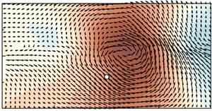
Contour maps of conditional average statistics along with the cross-sectional velocity vector for  $s/h=0.2$: (a,c) results with the reference point
 $(x,y,z) = (L_x/2, 10\nu /u_\tau, L_z/2)$; (b,d) results with the reference point (
 $L_x/2, -0.2H, L_z/2$). Panels (a,b) show the pressure fluctuations, and (c,d) show the temperature fluctuations. The reference point is denoted by an open circle.

4. Conclusions
To study the favourable breakdown of the Reynolds analogy by the spanwise rollers associated with the K–H instability, we performed DNS of turbulent heat transfer over high-aspect-ratio streamwise-aligned longitudinal ribs at the friction Reynolds number  $300$. The temperature was assumed as a passive scalar with Prandtl number unity to discuss the similarity between the heat and momentum transfer. The high-aspect-ratio longitudinal ribs lead to the favourable breakdown of the Reynolds analogy, that is, the Reynolds analogy factor exceeds unity. The maximum Reynolds analogy factor
 $RA=1.45$ is attained when the separation between the neighbouring ribs is
 $0.2$ times as large as the rib height. The favourable breakdown of the Reynolds analogy is dominantly attributed to the enhanced turbulent heat flux compared with the Reynolds shear stress, whereas the rib-induced secondary mean flow plays a role in diminishing the favourable breakdown of the Reynolds analogy. The conditional average statistics reveals that the high-pressure region, which is accompanied by the spanwise rollers, suppresses the sweep and ejection motions, which results in the smaller Reynolds shear stress than the turbulent heat flux.
In this study, only flows with a single Prandtl number at a single Reynolds number were considered, and the solid rib ideally has a constant wall temperature with the assumption of the infinite conductivity. However, considering that the spanwise rollers associated with K–H instability, which primarily cause the favourable breakdown of the Reynolds analogy, develop over various types of porous walls at various Reynolds numbers, the passive flow control by spanwise rollers may be used in numerous practical applications. In addition, there is probably room for improvement of the heat transfer performance in the geometric configuration of the ribs, which will be the focus of our future work.
Funding
The author expresses their gratitude to their colleagues PhD K. Suga and Dr M. Kaneda for their support. A part of this study was supported financially by JSPS Japan (no. 21H01266). The numerical calculations were carried out on the TSUBAME3.0 supercomputer in the Tokyo Institute of Technology.
Declaration of interests
The author reports no conflict of interest.



