Laser tracker-based surface measurement of antenna

The measurement schematic based on the laser tracker to detect the surface of the antenna is shown in Fig. 1.

Figure 1.

Measurement schematic for detecting the surface of antenna based on laser tracker.

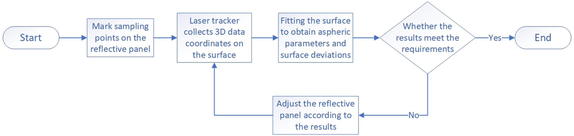
First of all, determine the sampling interval and mark the sampling point according to the size and shape of the panel. The spherically mounted retroreflector (SMR) is positioned on the marked sampling points after the laser tracker has been benchmarked. The corner cube prism inside the SMR reflects the laser from the laser tracker back in the original direction, allowing the coordinate data of the sampling points to be recorded. After sampling the 3D coordinates of the points on the panel, the aspherical parameters and surface deviations of the reflective panel can be fitted using the SF-DMC method investigated in this paper. Eventually, the position and internal deviation of sub-panels can be adjusted in accordance with the fitting results. The specific process is shown in Fig. 2.

Figure 2.

Flowchart of the surface measurement of antenna reflector panel.

Fundamentals of the SF-DMC method

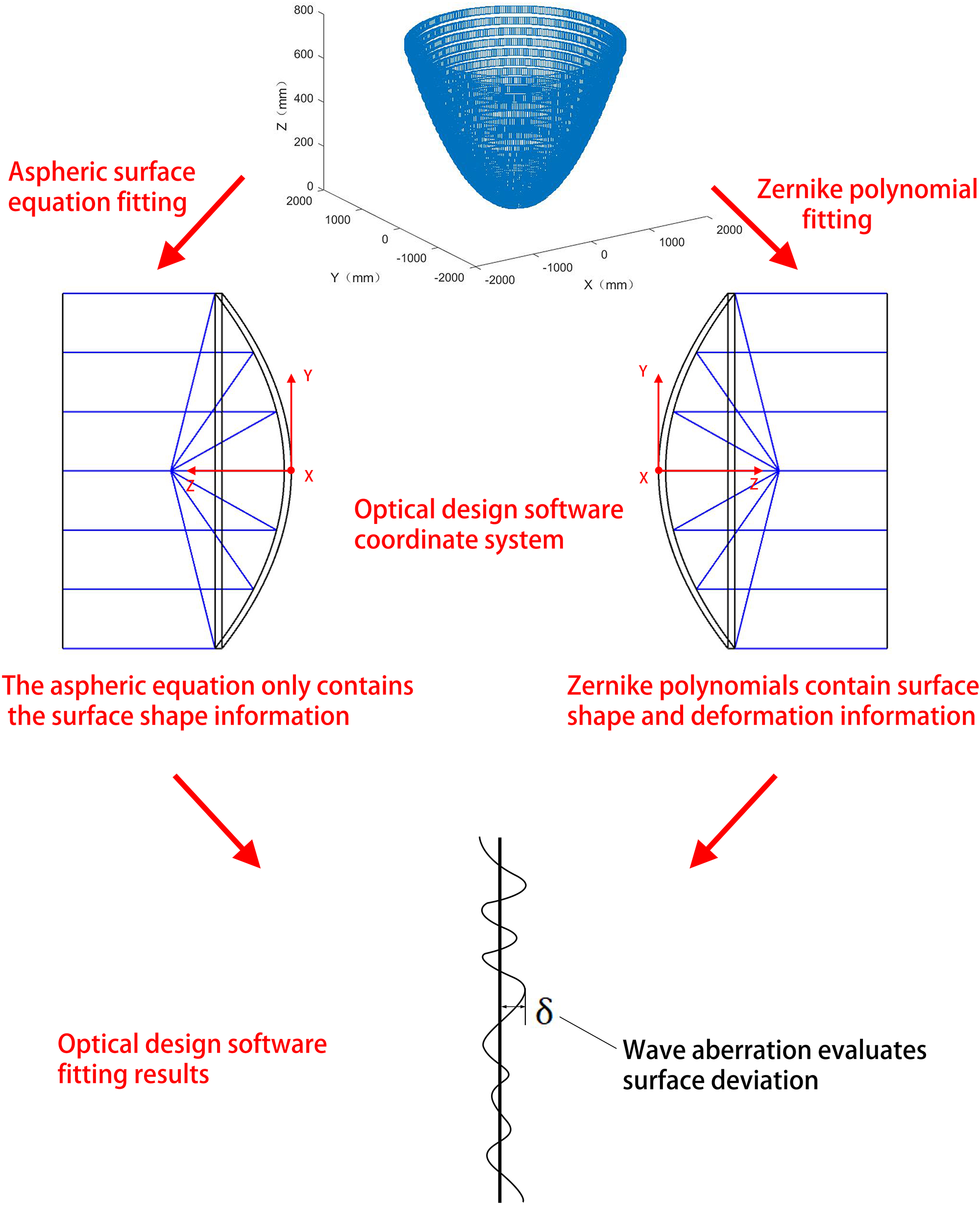
The SF-DMC method is proposed for obtaining the antenna’s aspherical surface parameters and evaluating its surface accuracy. The principle is shown in Fig. 3. The surface to be measured is characterized by two models: the asphere equation and the Zernike polynomial. The optical design software is then utilized to optimize the difference between the two expressions above and obtain the parameters and deviations of the surface to be measured.

Figure 3.

The schematic diagram of surface fitting principle.

The 3D coordinate dataset (x, y, z) measured by the laser tracker can be fitted with Zernike polynomials:

(1)\begin{equation}\bar Z\left( {r,\,\theta } \right) = \mathop \sum \limits_{k = 0}^n {A_k}{Z_k}\left( {r,\,\theta } \right)\end{equation}

where $\bar Z\left( {r,{ }\theta } \right)$ is the vertical height measured on the surface of the asphere. The ${A_k}$ in the above formula denotes the coefficient of each term of the Zernike polynomials. The $r = \sqrt {\left( {{x^2} + {y^2}} \right)} $ denotes the horizontal distance of the point measured on the surface of the asphere from the origin. The $\theta = {\text{actan}}\left( {y/x} \right)$ denotes the angle on the horizontal plane with respect to the origin. The n denotes the total number of terms in the Zernike polynomials. Also, any aspherical surface can be characterized by the aspherical surface equation [Reference Pan13]:

(2)\begin{align}z &= \left( {{r^2}/{R_0}} \right)/\left( {1 + \sqrt {1 - \left( {K + 1} \right){{\left( {x/{R_0}} \right)}^2}} } \right) \nonumber\\ &\quad + {a_1}{r^2} + {a_2}{r^4} + {a_3}{r^6} + {a_4}{r^8} + {a_5}{r^{10}} + \ldots \end{align}

where z is the vertical height of the point on the surface of the aspherical element measured from the origin. The ${R_0}$ denotes the radius of curvature of the aspherical element. The K denotes the conic coefficient. The ${a_1}$, ${a_2}$, ${a_3}$, ${a_4}$, and ${a_5}$ denote the higher order coefficients. After getting the aspherical parameters, the surface deviation can be calculated using the following equation:

(3)\begin{equation}\delta = \bar Z\left( {r,\,\theta } \right) - z\left( {{R_0},\,K,\,{a_1},\,{a_2},\,{a_3}\ldots} \right)\end{equation}

In optical design software, a difference model δ is generated based on two surface representations: the aspherical equation and the Zernike polynomials. The difference model is equivalent to an ideal plane when these two representations characterize the same ideal surface but have opposite z directions. As the aspherical surface to be measured has surface deviations or the feature parameters of the processed surface stray from the design values, the difference model will, therefore, deviate from the plane. The Levenberg–Marquardt algorithm (LMA) performs the optimization iteration by minimizing deviations to search for the aspherical parameters that are closest to the aspherical surface to be tested. This allows for the aspherical parameters to be acquired [Reference Marquardt14]. Finally, the surface deviations can be obtained from Equation (3). The specific flow is shown in Fig. 4.

Figure 4.

Flowchart of surface fitting.

Emulation verification and scope of application analysis

In order to verify the feasibility of this research method, an aspherical surface with known parameters is constructed based on Equation (2) for surface fitting. The difference model δ is established in the optical design software based on the two surface representations: aspherical equations and Zernike polynomials. The Zernike polynomial coefficients are calculated by converting the 3D coordinate data from the simulated model. The simulation was run for different values of the conic coefficient K, with the initial radius of curvature of the simulated objects set at 2048 mm. Through the optimization iteration of the LMA, the aspherical parameters R0 and K, which are closest to the aspherical elements to be tested, can be searched for.

The simulation results using 66-term Zernike polynomials are shown in Fig. 6, where the maximum deviation percentage of the radius of curvature in the range of −4 ≤ K ≤ 0.3 is 0.036%, the deviation percentage of the conic coefficient is 0.14%, and the RMS and Peak to Valley (PV) are 0.1505 mm and 0.7652 mm, respectively. As shown in Fig. 5, the paraboloid has the best fitting results, with almost no deviation; for the other aspherical surfaces, the closer to the paraboloid, the better the aspherical surface is fitted. Thus, this method works well for fitting paraboloid-type antennas. Furthermore, depending on the scope of application of K, it can also be used for fitting spherical-type antennas and other antennas with large hyperboloidal or ellipsoidal secondary mirrors [Reference Castleberg and Xilouris15–Reference Bolli, Orlai, Stringhetti, Orfei, Righini, Ambrosini, Bartolini, Bortolini, Bortolotti, Fiocchi, Gaudiomonte, Maccaferri, Mariotti, Marongiu, Melis, Migoni, Morsiani, Nanni, Nasyr, Pellizzoni, Pisanu, Poloni, Poppi, Porceddu, Prandoni, Roda, Roma, Scalambra, Serra, Trois, Valente, Vargiu and Zacchiroli17].

Figure 5.

Parabolic surface fitting data cloud and surface deviation.

Figure 6.

The fitting results of the aspherical parameters with the change of the cone coefficient.

Additionally, a simulation is conducted to evaluate the fitting accuracy between the 36-term Zernike polynomials and the 66-term Zernike polynomials. Figure 6 displays that the 36-term Zernike polynomial fitting also works well for paraboloid, but the RMS and PV for the remaining aspherical surfaces are worse than the 66-term Zernike polynomial fit. Therefore, when fitting the complicated aspherical surface, the 66-term Zernike polynomial fit is recommended.

Analysis of key factors

Effect of measurement errors

When sampling the antenna panel, the manual sampling process, as well as the instrument’s accuracy, will cause errors in the data. Therefore, it is necessary to analyze the error’s order of magnitude. As can be seen in Table 1, the laser tracker utilized in this study, the API Radiant Core, has a measurement error of 0.015 mm; the manually measured error is approximately 0.02 mm; and the roughness of the surfaces for most antennas is typically between a few and a dozen micrometers [Reference Gao18]. Consequently, the study assumes a normal distribution for random measurement errors with a variance of ±0.1 mm.

Table 1.

Key parameters of radian core laser tracker

Depending on the source of mistakes, random errors are added to the simulation data in all three directions (X, Y, and Z) to investigate the impact of measurement errors on simulation fitting results. For this purpose, a parabolic element with a radius of curvature R of 2048 mm and a conic coefficient K of −1 is constructed using Equation (2) for discussion.

The Zernike polynomials are more effective only with continuous data, and the high-frequency errors lead to their higher-order coefficients being abnormally large. In that case, it is more accurate to choose fewer terms to fit as long as the quantity of data points is high enough. Therefore, we compared the 36-term and 66-term Zernike polynomial fits, respectively, and the number of data points used in the simulation is 81 × 81. As indicated by Fig. 7, the deviation of the radius of curvature from the initial design value and the RMS fitting results grow as the error increases, and the fitting with 36-term Zernike polynomials is more accurate. When the random error is 0.1 mm, the percentage deviation of the radius and RMS fitting results are 0.00057% and 0.009 mm, respectively.

Figure 7.

The fitting results of curvature radius and RMS under different random errors.

Analysis of sampling influences

Number of samples

We adjust the number of samples for fitting from roughly 10²–10⁶, with a random error of 0.05 mm. As displayed in Fig. 8, the deviation of its radius of curvature fitting results decreases significantly with the increase in sample size, and we conclude that the data points must be guaranteed to be above 10³ to ensure their accuracy. When the number of sampling points is 1681, the percentage deviation of the radius of curvature and the RMS fitting results fitted by 36-term Zernike polynomials are 0.00065% and 0.0169 mm, respectively. And when the number of sampling points is 196, the percentage deviation of the radius of curvature and the RMS fitting results are 0.0126% and 0.0507 mm. Although the error increases, the fitting method is accurate enough for millimeter-wave band antennas. Therefore, this method can be used in the case of different sampling points. More sampling points correspond to the sub-millimeter-wave band, and fewer sampling points correspond to the millimeter-wave band.

Figure 8.

Fitting results of curvature radius and RMS with the number of sampling points.

Sampling distribution

In practice, antennas are usually sampled along radial and tangential directions, as shown in Fig. 9(b), rather than uniformly in the simulation above. Therefore, simulation studies were conducted for different sampling distributions and repeated five times to rule out the serendipity of the data while maintaining the same sample size and noise level. The simulation results are shown in Fig. 10. The RMS of the 36-term Zernike polynomial fitting results is smaller compared with the 66-term, and the difference in results is not significant between uniform and radial sampling. The maximum surface deviation RMS is 0.0092 mm, and the percentage of radius of curvature deviation is 0.0032% when adopting the radial distribution for sampling.

Figure 9.

Sampling distribution: (a) uniform sampling and (b) radial sampling.

Figure 10.

Fitting results of radius of curvature and RMS under different sampling distributions.

Subjects and measurement process

In this paper, our main implementation object of the surface fitting method is the Antarctic 3.2 m-aperture millimeter-wave radio telescope. As shown in Fig. 11, the antenna is of the parabolic type, with an all-aluminum receiving surface and a radius of curvature designed at 2048 mm.

Figure 11.

Design of 3.2 m splicing radio antenna.

Because of the large aperture sector antenna’s processing technique, cost, and other constraints, it cannot be employed in a one-piece structure, necessitating the use of a multi-panel structural combination. The number of sub-panels affects the complexity of the back-frame support structure and antenna performance, and the processing accuracy diminishes as panel area increases [Reference Qian, Wen, Wang and Lin19]. Taking the above factors into account, the antenna measured in this paper adopts 12 pieces of rotationally symmetric sector sub-panel splicing. For the design characteristics of this telescope, we adopt the laser tracker interferometric distance measurement method, which can realize high-precision measurement in a wide range.

As shown in Fig. 12, each sub-panel of the antenna is sequentially measured with a laser tracker. Every 5 cm along the tangential direction, samples are taken and marked on the panel’s surface. The target ball is placed in the position of the marker to reflect back the laser tracker-emitted laser, allowing the 3D coordinates of the data at each point to be acquired $\left( {{x_1},{y_1},{z_1}} \right),\left( {{x_2},{y_2},{z_2}} \right), \ldots ,\left( {{x_i},{y_i},{z_i}} \right)$.

Figure 12.

The process of antenna measurement based on laser tracker.

Surface fitting results

Repeated measurements and fitting results

When we apply the methods studied in this paper to fit the 3.2 m radio telescope, the 36-term Zernike polynomials are adopted due to the influence of manual error in coordinate data. Since the discrete point data are sensitive to the step signal, the data of the laser tracker are used to adjust the panel splicing. The fitted surface deviation distribution is used to adjust the internal surface of the single panel. Then the panel is fitted into an aspheric surface for subsequent fixed focus mounting. Subsequently, further debugging is carried out until the radio telescope’s accuracy meets the design specification.

The results are shown in Fig. 13; a total of eight sets of data are measured with the telescope aperture placed facing upward. We employ two types of fitting ways in the experiment: aspherical fit with an unknown cone factor and radius of curvature, and parabolic fit with an unknown radius of curvature. The aspherical fit is used to evaluate the similarity between the antenna’s surface under test and the paraboloid, and the paraboloidal fit is used to detect the deviation of the surface between the antenna’s surface and the ideal paraboloid. As can be seen in Fig. 13, the values of the radius of curvature stabilize as the panel is rectified, the conic coefficient values tend to −1, and the RMS and PV values follow a synchronized downward trend. In the final set of measurements, the paraboloidal fit’s radius of curvature is 2032.3839 mm, the RMS is 0.8407 mm, and the PV is 6.5377 mm. The asphere fit’s radius of curvature is 2012.3204 mm, the conic coefficient is −1.0476, the RMS is 0.6232 mm, and the PV is 6.5353 mm. The RMS for the aspherical fit decreased by about 61.84% compared with the first measurement. Since the antenna needs to adjust the sub-panel continuously in order to reduce surface deviation, its final radius of curvature is not always consistent with the theoretical design value, and the change in surface deviation during the measurement process is shown in Fig. 14.

Figure 13.

The fitting results of the surface in the adjustment process of the telescope panel.

Figure 14.

The surface deviation variation of aspherical fitting in the adjustment process of the telescope panel.

Measurements with different telescope attitudes

During the actual measurement, the telescope needs to be adjusted to align with the celestial bodies to be observed. However, while adjusting its orientation, the telescope’s surface may change due to gravity, airflow, and other factors. Therefore, this experiment investigates the effects of positioning the telescope horizontally and obliquely at 80°. These two telescope attitudes are shown in Fig. 15.

Figure 15.

Different attitudes of radio telescopes: (a) placed horizontally and (b) placed obliquely at 80°.

The percentage deviations of different parameters provided in Table 2 indicate that the telescope panel is susceptible to external variables such as gravity, and the RMS and PV are more sensitive due to their smaller order of magnitude. The reason for these results may be that there are gaps in the splicing between each sub-panel, which cause it to shift and tilt when the telescope changes its attitude. Apart from this, the thin panels and large aperture of the telescope also make it more sensitive to gravity. The surface deviations of the two attitude parabolic fits are shown in Fig. 16.

Table 2.

Aspherical surface fitting results of different attitudes of radio telescopes

Figure 16.

The surface deviation of spherical surface fitting under different attitudes of telescope: (a) placed horizontally and (b) placed obliquely at 80°.

By fitting and correcting the panels, we can control the surface deviation of the telescope at 0.6232 mm. As Fig. 17 shows, we have successfully transported the radio telescope to the South Pole for observation, thereby verifying the feasibility of the present study’s method. The impact of different factors on the experimental results will be discussed below.

Figure 17.

3.2 m radio telescope (left) transported to the Antarctic site.