1 Introduction
The hydrodynamic interaction of a sphere moving in the vicinity of a plane wall constitutes a classic problem of fluid mechanics (Lorentz Reference Lorentz and Lorentz1907; Faxen Reference Faxen1923; Brenner Reference Brenner1961; Maude Reference Maude1961; O’Neill Reference O’Neill1964; Goldman, Cox & Brenner Reference Goldman, Cox and Brenner1967; O’Neill & Stewartson Reference O’Neill and Stewartson1967; Goren Reference Goren1973; Happel & Brenner Reference Happel and Brenner1983; Loussaief, Pasol & Feuillebois Reference Loussaief, Pasol and Feuillebois2015). It has an impact on the dynamics of settling, Brownian motion and collision or deposition kinetics of particles at walls. For Stokes flow with no-slip boundary conditions, the hydrodynamic force on a sphere of radius  $R$ approaching a plane wall at constant velocity
 $U$ in the normal direction diverges inversely proportional to the width
 $H$ of the gap (Hocking Reference Hocking1973). Due to the finite mean free path
 $\ell$ of gas molecules it is clear that this classic approach poses an approximation in the gas phase which must be refined by taking into account velocity slip at small Knudsen numbers,
 $Kn=\ell /R\lesssim 0.1$. For larger
 $Kn$, however, the Stokes equation loses its validity and must be replaced by the Boltzmann equation.
In the slip-flow regime the movement of a sphere close to a wall was investigated using a Navier-slip condition (Goren Reference Goren1973; Hocking Reference Hocking1973; Vinogradova Reference Vinogradova1995; Luo & Pozrikidis Reference Luo and Pozrikidis2008) or following the singular perturbation scheme of Sone & Onishi (Reference Sone and Onishi1978) in Ying & Peters (Reference Ying and Peters1989, Reference Ying and Peters1991). In this case a much weaker logarithmic divergence of the force on the width of the gap is found on close approach, but these results are limited to non-overlapping Knudsen layers,  $\ell \ll H$, in the gap. For small gap widths, Sundararajakumar & Koch (Reference Sundararajakumar and Koch1996) provide a non-continuum lubrication approximation based on results of Cercignani & Daneri (Reference Cercignani and Daneri1963) for the flow of a rarefied gas between parallel plates. This analysis is valid for
 $Kn=\ell /R\ll \sqrt{H/R}\ll 1$, while a less rigorous argument is employed to extend the result to cases with a narrow gap at large
 $Kn$. The hydrodynamic interaction of a sphere with a plane wall in free molecular and transition regimes is yet to be addressed.
There is a significant overlap between the analysis of the motion of a single particle near a wall and particle–particle interactions. Many of the treatments in the slip-flow regime mentioned in the previous paragraph contain an analysis of the relative motion between two spheres. Gopinath & Koch (Reference Gopinath and Koch1997, Reference Gopinath and Koch1999) have investigated the interaction between spheres and cylinders in the free molecular regime through an integral equation formalism. Ramanathan, Koch & Bhiladvala (Reference Ramanathan, Koch and Bhiladvala2010) have calculated the drag force on a cylinder vibrating normal to a plane wall using analytical techniques in both the free molecular and slip-flow regimes as well as Bhatnagar–Gross–Krook-based low-Mach-number direct simulation Monte Carlo (DSMC) treatments for intermediate Knudsen numbers. They provide a fit function for the drag force on a wire in the whole range of  $Kn$.
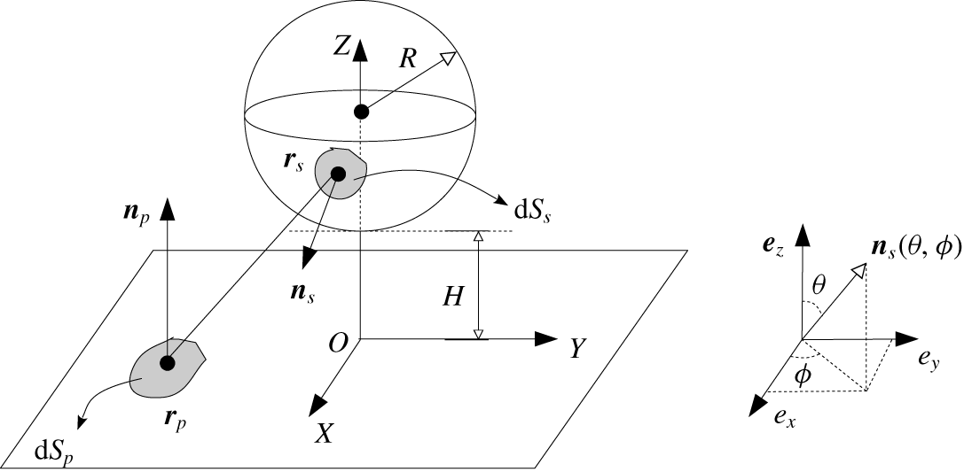
In this article, we quantify the free molecular drag force on a spherical particle moving normal and tangential to a plane wall (see figure 1). We employ an integral-equation-based approach to obtain the drag force, assuming isothermal conditions and diffuse reflection at walls. This analysis is compared to and complemented by DSMC results, extending the study to the transition flow regime.
Sketch of the geometry. A sphere of radius  $R$ is located with its centre at a distance
 $D=R+H$ above the plane
 $Z=0$. Points on the plane are parameterized by
 $\boldsymbol{r}_{p}=X\boldsymbol{e}_{x}+Y\boldsymbol{e}_{y}$ and points on the sphere by
 $\boldsymbol{r}_{s}=D\boldsymbol{e}_{z}+R\boldsymbol{n}_{s}(\unicode[STIX]{x1D703},\unicode[STIX]{x1D719})$, where
 $\boldsymbol{n}_{p}=\boldsymbol{e}_{z}$ and
 $\boldsymbol{n}_{s}(\unicode[STIX]{x1D703},\unicode[STIX]{x1D719})=\boldsymbol{e}_{x}\sin \unicode[STIX]{x1D703}\cos \unicode[STIX]{x1D719}+\boldsymbol{e}_{y}\sin \unicode[STIX]{x1D703}\sin \unicode[STIX]{x1D719}+\boldsymbol{e}_{z}\cos \unicode[STIX]{x1D703}$ are the unit normals on the plane and sphere, respectively.

2 Theoretical framework
A spherical particle of radius  $R$, whose centre is located at a height
 $(R+H)$ above the
 $XOY$ plane, is moving at a velocity
 $\boldsymbol{U}$ in a direction either normal
 $(\boldsymbol{U}=-U\boldsymbol{e}_{z})$ or parallel
 $(\boldsymbol{U}=U\boldsymbol{e}_{x})$ to the plane (figure 1). The motion of rarefied gas induced by the moving sphere is governed by the Boltzmann equation, which in the absence of any external force reads
 $$\begin{eqnarray}\frac{\unicode[STIX]{x2202}(nf)}{\unicode[STIX]{x2202}t}+\boldsymbol{c}\boldsymbol{\cdot }\unicode[STIX]{x1D735}_{r}(nf)=J\left(nf,nf\right),\end{eqnarray}$$
where  $f(\boldsymbol{r},\boldsymbol{c},t)$ is the velocity distribution function of the gas molecules,
 $\boldsymbol{c}$ is the molecular velocity,
 $\boldsymbol{r}$ is the position vector,
 $t$ is time,
 $n(\boldsymbol{r},t)$ is the molecular number density and
 $J(nf,nf)$ represents intermolecular collisions, which are neglected in the free molecular regime. Let
 $n\sim n_{\infty }$,
 $\boldsymbol{c}\sim \bar{c}$,
 $t\sim R/U$ and
 $\boldsymbol{r}\sim R$ be characteristic scales for the respective variables, where
 $\bar{c}=\sqrt{2kT/m}$ is the most probable thermal velocity of gas molecules,
 $k=1.380649\times 10^{-23}$ J K
 $^{-1}$ is the Boltzmann constant,
 $T$ is the temperature,
 $m$ is the molecular mass and
 $n_{\infty }$ is the number density far away from the plane. Using non-dimensional variables based on this scaling the collisionless Boltzmann equation becomes
 $Sh\,\unicode[STIX]{x2202}_{\tilde{t}}({\tilde{n}}f)+\tilde{\boldsymbol{c}}\boldsymbol{\cdot }\unicode[STIX]{x1D735}_{\tilde{r}}({\tilde{n}}f)=0$, where
 $Sh=U/\bar{c}$ is the Strouhal number (closely related to the Mach number) and a tilde indicates the respective non-dimensional quantity. Expanding the distribution function in
 $Sh$ as
 $({\tilde{n}}f)=({\tilde{n}}f)^{(0)}+Sh({\tilde{n}}f)^{(1)}+\cdots \,$, where
 $({\tilde{n}}f)^{(0)}$ corresponds to the stationary and homogeneous Maxwellian distribution for a sphere at rest, shows that to
 $O(Sh)$ the Boltzmann equation (2.1) without collision term reduces to the quasi-stationary expression
 $$\begin{eqnarray}\boldsymbol{c}\boldsymbol{\cdot }\unicode[STIX]{x1D735}_{r}(nf)=0.\end{eqnarray}$$
The molecular distribution function  $(nf)$ at some position
 $\boldsymbol{r}_{0}$ can thus be obtained by tracing back the trajectory of a molecule along the ray (or characteristic)
 $\boldsymbol{r}=(\boldsymbol{r}_{0}-\boldsymbol{c}s)$,
 $s>0$, until a boundary is reached where the distribution function is known. In the present case molecules either will come from the far field, where the velocity distribution function is assumed to be a Maxwellian,
 $$\begin{eqnarray}f_{M}(\boldsymbol{c})=\left(\frac{m}{2\unicode[STIX]{x03C0}kT}\right)^{3/2}\exp \left(-\frac{m}{2kT}\left|\boldsymbol{c}\right|^{2}\right),\end{eqnarray}$$
with number density  $n_{\infty }$, or will originate from the surface of the sphere or the plane. In the case of molecules having been reflected, a Maxwellian velocity distribution in the respective inertial frame of reference moving with the scattering surface and a position-dependent number density
 $n(\boldsymbol{r})$ applies.
To obtain the molecular number densities on the sphere and plane, we employ the flux conservation equation assuming that both surfaces are impermeable and no adsorption occurs. Therefore, at any point on the sphere or plane, the flux of incident molecules equals the flux of reflected molecules:
 $$\begin{eqnarray}j_{s}^{in}(\boldsymbol{r}_{s})=j_{s}^{out}(\boldsymbol{r}_{s}),\quad j_{p}^{in}(\boldsymbol{r}_{p})=j_{p}^{out}(\boldsymbol{r}_{p}),\end{eqnarray}$$
where the subscripts  $s$ and
 $p$ are for the sphere and the plane, respectively, and
 $\boldsymbol{r}_{s}$ and
 $\boldsymbol{r}_{p}$ are positions on these surfaces. For diffuse reflection, molecules reflected from the surface of the sphere have their velocities distributed according to
 $f_{M}(\boldsymbol{c}-\boldsymbol{U})$, while molecules reflected from the plane obey the velocity distribution
 $f_{M}(\boldsymbol{c})$. With the number densities
 $n_{s}(\boldsymbol{r}_{s})$ and
 $n_{p}(\boldsymbol{r}_{p})$, the outgoing fluxes of molecules reflected from the sphere and plane are
 $$\begin{eqnarray}\displaystyle & \displaystyle j_{s}^{out}(\boldsymbol{r}_{s})=n_{s}(\boldsymbol{r}_{s})\int _{(\boldsymbol{c}-\boldsymbol{U})\boldsymbol{\cdot }\boldsymbol{n}_{s}>0}|(\boldsymbol{c}-\boldsymbol{U})\boldsymbol{\cdot }\boldsymbol{n}_{s}|\,f_{M}(\boldsymbol{c}-\boldsymbol{U})\,\text{d}\boldsymbol{c}=\unicode[STIX]{x1D706}n_{s}(\boldsymbol{r}_{s}), & \displaystyle\end{eqnarray}$$
 $$\begin{eqnarray}\displaystyle & \displaystyle j_{p}^{out}(\boldsymbol{r}_{p})=n_{p}(\boldsymbol{r}_{p})\int _{\boldsymbol{c}\boldsymbol{\cdot }\boldsymbol{n}_{p}>0}|\boldsymbol{c}\boldsymbol{\cdot }\boldsymbol{n}_{p}|\,f_{M}(\boldsymbol{c})\,\text{d}\boldsymbol{c}=\unicode[STIX]{x1D706}n_{p}(\boldsymbol{r}_{p}), & \displaystyle\end{eqnarray}$$
where  $\boldsymbol{n}_{s}$ and
 $\boldsymbol{n}_{p}$ are unit normal vectors on the surface of the sphere and plane pointing into the gas phase and
 $\unicode[STIX]{x1D706}=\bar{c}/(2\sqrt{\unicode[STIX]{x03C0}})$. The flux due to incident molecules on the sphere
 $j_{s}^{in}(\boldsymbol{r}_{s})$ (or plane
 $j_{p}^{in}(\boldsymbol{r}_{p})$) consists of two components, one due to far-field molecules and one due to molecules reflected from the plane (or sphere):
 $$\begin{eqnarray}\displaystyle j_{s}^{in}\left(\boldsymbol{r}_{s}\right) & = & \displaystyle n_{\infty }\int _{\left(\boldsymbol{c}-\boldsymbol{U}\right)\boldsymbol{\cdot }\boldsymbol{n}_{s}<0}\left|\left(\boldsymbol{c}-\boldsymbol{U}\right)\boldsymbol{\cdot }\boldsymbol{n}_{s}\right|f_{M}\left(\boldsymbol{c}\right)\text{d}\boldsymbol{c}-n_{\infty }\int _{\unicode[STIX]{x1D6FA}_{ps}}|(\boldsymbol{c}-\boldsymbol{U})\boldsymbol{\cdot }\boldsymbol{n}_{s}|f_{M}(\boldsymbol{c})\,\text{d}\boldsymbol{c}\nonumber\\ \displaystyle & & \displaystyle +\,\int _{\unicode[STIX]{x1D6FA}_{ps}}\left|\left(\boldsymbol{c}-\boldsymbol{U}\right)\boldsymbol{\cdot }\boldsymbol{n}_{s}\right|n_{p}(\boldsymbol{r}_{p})f_{M}(\boldsymbol{c})\,\text{d}\boldsymbol{c},\end{eqnarray}$$
 $$\begin{eqnarray}\displaystyle j_{p}^{in}\left(\boldsymbol{r}_{p}\right) & = & \displaystyle n_{\infty }\int _{\boldsymbol{c}\boldsymbol{\cdot }\boldsymbol{n}_{p}<0}|\boldsymbol{c}\boldsymbol{\cdot }\boldsymbol{n}_{p}|\,f_{M}\left(\boldsymbol{c}\right)\text{d}\boldsymbol{c}-n_{\infty }\int _{\unicode[STIX]{x1D6FA}_{sp}}|\boldsymbol{c}\boldsymbol{\cdot }\boldsymbol{n}_{p}|\,f_{M}(\boldsymbol{c})\,\text{d}\boldsymbol{c}\nonumber\\ \displaystyle & & \displaystyle +\,\int _{\unicode[STIX]{x1D6FA}_{sp}}|\boldsymbol{c}\boldsymbol{\cdot }\boldsymbol{n}_{p}|n_{s}(\boldsymbol{r}_{s})f_{M}(\boldsymbol{c}-\boldsymbol{U})\,\text{d}\boldsymbol{c}.\end{eqnarray}$$
Here  $\unicode[STIX]{x1D6FA}_{ps}$ denotes the solid angle under which molecules emanating from the plane reach the point
 $\boldsymbol{r}_{s}$ on the sphere (implying
 $(\boldsymbol{c}-\boldsymbol{U})\boldsymbol{\cdot }\boldsymbol{n}_{s}<0$ in the integrals), whereas
 $\unicode[STIX]{x1D6FA}_{sp}$ is the solid angle under which reflected molecules from the sphere reach the point
 $\boldsymbol{r}_{p}$ on the plane (implying
 $\boldsymbol{c}\boldsymbol{\cdot }\boldsymbol{n}_{p}<0$ in the integrals). In both expressions the contribution from far-field molecules has been written as an integral over molecules impinging from all directions, while subtracting a correction due to regions screened by the plane and sphere, respectively.
The motion of the sphere induces a small modification,  $\unicode[STIX]{x1D708}_{i}\sim O(Sh)$, of the number densities
 $n_{i}(\boldsymbol{r}_{i})=n_{\infty }(1+\unicode[STIX]{x1D708}_{i}(\boldsymbol{r}_{i}))$, and the velocity distribution is expanded as
 $f_{M}(\boldsymbol{c}\mp \boldsymbol{U})\approx f_{M}(\boldsymbol{c})\{1\pm (m/kT)\boldsymbol{c}\boldsymbol{\cdot }\boldsymbol{U}\}$ to first order in
 $Sh$ whenever required. Using these expressions in (2.7) and (2.8), we obtain integral equations for the excess molecular densities
 $\unicode[STIX]{x1D708}_{s}(\boldsymbol{r}_{s})$ on the sphere and
 $\unicode[STIX]{x1D708}_{p}(\boldsymbol{r}_{p})$ on the plane to first order in
 $Sh$ as
 $$\begin{eqnarray}\displaystyle & \displaystyle \unicode[STIX]{x1D706}\unicode[STIX]{x1D708}_{s}(\boldsymbol{r}_{s})=-\frac{3}{4\unicode[STIX]{x03C0}}\int _{\boldsymbol{e}_{w}\boldsymbol{\cdot }\boldsymbol{n}_{s}<0}|\boldsymbol{e}_{w}\boldsymbol{\cdot }\boldsymbol{n}_{s}|(\boldsymbol{e}_{w}\boldsymbol{\cdot }\boldsymbol{U})\,\text{d}\unicode[STIX]{x1D6FA}_{w}+\frac{\unicode[STIX]{x1D706}}{\unicode[STIX]{x03C0}}\int _{\unicode[STIX]{x1D6FA}_{ps}}|\boldsymbol{e}_{w}\boldsymbol{\cdot }\boldsymbol{n}_{s}|\unicode[STIX]{x1D708}_{p}(\boldsymbol{r}_{p})\,\text{d}\unicode[STIX]{x1D6FA}_{w}, & \displaystyle\end{eqnarray}$$
 $$\begin{eqnarray}\displaystyle & \displaystyle \unicode[STIX]{x1D706}\unicode[STIX]{x1D708}_{p}(\boldsymbol{r}_{p})=\frac{3}{4\unicode[STIX]{x03C0}}\int _{\unicode[STIX]{x1D6FA}_{sp}}\left|\boldsymbol{e}_{c}\boldsymbol{\cdot }\boldsymbol{n}_{p}\right|\left(\boldsymbol{e}_{c}\boldsymbol{\cdot }\boldsymbol{U}\right)\,\text{d}\unicode[STIX]{x1D6FA}_{c}+\frac{\unicode[STIX]{x1D706}}{\unicode[STIX]{x03C0}}\int _{\unicode[STIX]{x1D6FA}_{sp}}\left|\boldsymbol{e}_{c}\boldsymbol{\cdot }\boldsymbol{n}_{p}\right|\unicode[STIX]{x1D708}_{s}(\boldsymbol{r}_{s})\,\text{d}\unicode[STIX]{x1D6FA}_{c}. & \displaystyle\end{eqnarray}$$
For points  $\boldsymbol{r}_{s}$ and
 $\boldsymbol{r}_{p}$ on the sphere and plane, the unit vectors
 $\boldsymbol{e}_{c}$ and
 $\boldsymbol{e}_{w}$ are
 $\boldsymbol{e}_{c}=-\boldsymbol{e}_{w}=\boldsymbol{r}_{sp}/r_{sp}=(\boldsymbol{r}_{p}-\boldsymbol{r}_{s})/|\boldsymbol{r}_{p}-\boldsymbol{r}_{s}|$. As before, the integrals over the solid angles
 $\unicode[STIX]{x1D6FA}_{ps}$ and
 $\unicode[STIX]{x1D6FA}_{sp}$ imply
 $\boldsymbol{e}_{w}\boldsymbol{\cdot }\boldsymbol{n}_{s}<0$ and
 $\boldsymbol{e}_{c}\boldsymbol{\cdot }\boldsymbol{n}_{p}<0$, respectively.
Evaluating the integrals independent of  $\unicode[STIX]{x1D708}_{i}(\boldsymbol{r}_{i})$ and converting the integrals over solid angles into integrals over surface elements, the above equations can be put into the form
 $$\begin{eqnarray}\unicode[STIX]{x1D708}_{s}(\boldsymbol{r}_{s})=\frac{\sqrt{\unicode[STIX]{x03C0}}}{\bar{c}}(\boldsymbol{U}\boldsymbol{\cdot }\boldsymbol{n}_{s})+\frac{1}{\unicode[STIX]{x03C0}}\int _{\unicode[STIX]{x2202}P}\frac{\left|\left(\boldsymbol{r}_{sp}\boldsymbol{\cdot }\boldsymbol{n}_{s}\right)\left(\boldsymbol{r}_{sp}\boldsymbol{\cdot }\boldsymbol{n}_{p}\right)\right|}{r_{sp}^{4}}\unicode[STIX]{x1D708}_{p}\left(\boldsymbol{r}_{p}\right)\,\text{d}S_{p},\end{eqnarray}$$
 $$\begin{eqnarray}\displaystyle \unicode[STIX]{x1D708}_{p}(\boldsymbol{r}_{p}) & = & \displaystyle \frac{3}{2\unicode[STIX]{x03C0}}\frac{\sqrt{\unicode[STIX]{x03C0}}}{\bar{c}}\left\{\frac{2\unicode[STIX]{x03C0}}{3}\left(\sqrt{1-\frac{R^{2}}{D^{2}+\unicode[STIX]{x1D70C}^{2}}}\left[1+\frac{R^{2}(\unicode[STIX]{x1D70C}^{2}/2-D^{2})}{(D^{2}+\unicode[STIX]{x1D70C}^{2})^{2}}\right]-1\right)(\boldsymbol{U}\boldsymbol{\cdot }\boldsymbol{n}_{p})\right.\nonumber\\ \displaystyle & & \displaystyle +\,\left.\unicode[STIX]{x03C0}\sqrt{1-\frac{R^{2}}{D^{2}+\unicode[STIX]{x1D70C}^{2}}}\frac{R^{2}D(\boldsymbol{r}_{p}\boldsymbol{\cdot }\boldsymbol{U})}{(D^{2}+\unicode[STIX]{x1D70C}^{2})^{2}}\right\}+\frac{1}{\unicode[STIX]{x03C0}}\int _{\unicode[STIX]{x2202}S}\frac{|(\boldsymbol{r}_{sp}\boldsymbol{\cdot }\boldsymbol{n}_{s})(\boldsymbol{r}_{sp}\boldsymbol{\cdot }\boldsymbol{n}_{p})|}{r_{sp}^{4}}\unicode[STIX]{x1D708}_{s}(\boldsymbol{r}_{s})\,\text{d}S_{s},\nonumber\\ \displaystyle & & \displaystyle\end{eqnarray}$$
where  $D=R+H$,
 $\unicode[STIX]{x1D70C}^{2}=\boldsymbol{r}_{p}\boldsymbol{\cdot }\boldsymbol{r}_{p}$ and
 $\unicode[STIX]{x2202}P$ and
 $\unicode[STIX]{x2202}S$ are segments of the plane and sphere visible from
 $\boldsymbol{r}_{s}$ and
 $\boldsymbol{r}_{p}$, respectively. The first term on the right-hand side of (2.11) represents the excess number of molecules for a sphere moving in an unbounded rarefied gas, as first evaluated by Epstein (Reference Epstein1924). Equations (2.11) and (2.12) constitute a coupled pair of Fredholm integral equations for
 $\unicode[STIX]{x1D708}_{s}$ and
 $\unicode[STIX]{x1D708}_{p}$ which are solved iteratively.
The integrals were evaluated by discretizing the spherical surface with a homogeneous  $(2N+1)\times (2N+1)$ grid and the plane with an inhomogeneous
 $(2M+1)\times (2M+1)$ grid using the shape functions
 $x_{pj}=5\times 10^{-7}\text{sgn}(\bar{x}_{j})|\bar{x}_{j}|^{1.2}$,
 $y_{pj}=x_{pj}$ and
 $\bar{x}_{j}=-1+(j-1)/M$. For numerical calculation, we have chosen
 $M$ and
 $N$ sufficiently large and iterated the integral equations sufficient times, so that an accuracy of
 $\Vert \unicode[STIX]{x1D708}_{p,s}^{(l+1)}-\unicode[STIX]{x1D708}_{p,s}^{(l)}\Vert _{inf}<10^{-4}$ is achieved.
Once the molecular number density is known, all other quantities of interest follow. In particular, the force on the sphere is
 $$\begin{eqnarray}\boldsymbol{F}_{s}=\int _{\unicode[STIX]{x2202}S}\int m\boldsymbol{c}|(\boldsymbol{c}-\boldsymbol{U})\boldsymbol{\cdot }\boldsymbol{n}_{s}|n(\boldsymbol{r}_{s})f\left(\boldsymbol{c},\boldsymbol{r}_{s}\right)\,\text{d}\boldsymbol{c}\,\text{d}S,\end{eqnarray}$$
where the integral extends over the momenta of both incoming and outgoing molecules over the whole surface of the sphere. Details of the calculation are given in appendix A. The error in non-dimensional drag force obtained using the Fredholm integral equation approach is of the order of  $10^{-3}$.
3 Numerical method
We use a variant of the DSMC method (Bird Reference Bird1994) suggested by Nanbu (Reference Nanbu1980) and investigated in Babovsky & Illner (Reference Babovsky and Illner1989) and Neunzert & Struckmeier (Reference Neunzert and Struckmeier1995). This method is based on a time-splitting algorithm for the Boltzmann equation. In the first step, the collisionless Boltzmann equation is solved and the boundary conditions are applied. In the second step, local homogenization over cells is performed, and the spatially homogeneous Boltzmann equation is solved (i.e. the equation that only contains the time derivative and the collision term), where the solution of the first step is considered as the initial condition. Finally, an explicit Euler scheme is performed with a time-step restriction related to the Knudsen number. The main difference between the original DSMC method and its variant is the simulation of the collision process in each cell (see Cercignani, Illner & Pulvirenti (Reference Cercignani, Illner and Pulvirenti2013) for details). Throughout this work, the hard-sphere collision kernel is employed.
We consider a computational domain consisting of a sphere of radius  $R=0.1~\unicode[STIX]{x03BC}\text{m}$ immersed in a cube of side length
 $L=10R$ or a rectangular cuboid of twice this extension in the
 $z$ direction when motion normal to the plane is considered. The computational domain is divided into small cubes of side length smaller than the mean free path. For example, for
 $Kn=\infty$ each axis is subdivided into intervals of length
 $L/20$ and for
 $Kn=1$ into intervals of length
 $L/100$. The constant time step is chosen as
 $\unicode[STIX]{x0394}t=10^{-11}$ s for all Knudsen numbers. In each cell gas molecules are initialized according to a Maxwellian (2.3), with parameters given by the initial density, temperature and mean velocity. The method consists of two steps: a free molecular and a collision step. In the free molecular step gas molecules are propagated with their respective velocity over a time interval
 $\unicode[STIX]{x0394}t$. When gas molecules cross a boundary they are reflected or removed according to the boundary conditions. On solid-wall boundaries a diffuse reflection boundary condition is applied. A far-field boundary condition applies at the surface of the computational domain. It is implemented by generating gas molecules according to the Maxwellian (2.3) in the vicinity of the boundary cells, i.e. in ghost cells. For the case of a moving sphere, the sphere is translated together with the gas molecules in the free-flow step with the same time interval
 $\unicode[STIX]{x0394}t$ as for the gas molecules.
In order to compute the force on the sphere we sum over all incident and reflected molecules during the free-flow step. We obtain the drag force according to
 $$\begin{eqnarray}\boldsymbol{F}=\frac{m_{s}\displaystyle \mathop{\sum }_{i}(\boldsymbol{c}_{i}^{in}-\boldsymbol{c}_{i}^{ref})}{\unicode[STIX]{x0394}t},\end{eqnarray}$$
where  $m_{s}$ is the simulated mass (see Shrestha et al. (Reference Shrestha, Tiwari, Klar and Hardt2015) for details).
Three situations were considered, corresponding to a sphere moving through a virtually unbounded domain and motion parallel as well as normal to a wall. For the unbounded domain and motion parallel to the wall the simulations were performed in a frame of reference with the sphere at rest. By contrast, for the normal motion the wall determines the rest frame, with the sphere moving towards it. While the former cases are quasistatic and mean values of desired quantities are obtained by continuous integration based on the same simulation run, the latter case requires averaging over a large number of individual runs. The sphere is surrounded by a hard-sphere gas resembling argon of molecular mass  $m=6.63\times 10^{-26}~\text{kg}$ and diameter
 $d=3.68\times 10^{-10}~\text{m}$ (Sone Reference Sone2007) at temperature
 $T=300~\text{K}$ and number density
 $n=1/(\sqrt{2}\unicode[STIX]{x03C0}d^{2}\ell )$. The velocity of the sphere relative to the gas and wall was
 $50~\text{m}~\text{s}^{-1}$ throughout, corresponding to
 $Sh\approx 0.14$. It was verified that this is within the regime where the force scales linearly with
 $Sh$ to within the numerical accuracy. Note that with viscosity
 $\unicode[STIX]{x1D707}=(5/16)\sqrt{mkT/\unicode[STIX]{x03C0}}/d^{2}$ (Bird Reference Bird1994), the Reynolds number becomes
 $Re=2RU\unicode[STIX]{x1D70C}/\unicode[STIX]{x1D707}=32Sh/(5\sqrt{\unicode[STIX]{x03C0}}Kn)\approx 0.5/Kn$.
Drag on a spherical particle moving in an unbounded domain.

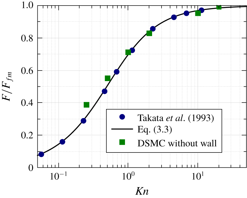
The method was tested for a spherical particle in an unbounded domain and compared to results reported in Takata, Sone & Aoki (Reference Takata, Sone and Aoki1993), obtained using the linearized Boltzmann equation with a hard-sphere collision model, in figure 2. There the drag force is shown normalized with the free molecular drag on a diffusely reflecting sphere at velocity  $U$, first calculated by Epstein (Reference Epstein1924):
 $$\begin{eqnarray}F_{fm}=\frac{\sqrt{\unicode[STIX]{x03C0}}}{3}(8+\unicode[STIX]{x03C0})R^{2}nm\sqrt{\frac{2kT}{m}}U.\end{eqnarray}$$
Included in the graph is a least-squares fit to the data of Takata et al. (Reference Takata, Sone and Aoki1993) by a rational function with quadratic polynomials in  $Kn$ in both numerator and denominator, exhibiting a linear increase at small
 $Kn$ and obeying the free molecular limit at large
 $Kn$:
 $$\begin{eqnarray}\frac{F}{F_{fm}}=\frac{0.657Kn+Kn^{2}}{0.420+0.957Kn+Kn^{2}}.\end{eqnarray}$$
This correlation agrees to better than 0.2 % with the results of Takata et al. (Reference Takata, Sone and Aoki1993) over the whole range of  $Kn$. We will use (3.3) as an estimate for the drag in an unbounded domain at finite
 $Kn$ in the following.
Excellent agreement between the DSMC results and the prediction by (3.3) is obtained for large  $Kn$, indicative of the fact that in the free molecular regime the distribution function for molecules impinging onto the sphere remains unaltered by the presence of the sphere. In the transition regime and below, the drag force is overestimated by the DSMC method. This is to be expected, as the flow around a sphere in the continuum and slip regime falls off slowly
 ${\sim}r^{-1}$ at large distances from the sphere, and the box used for DSMC simulation becomes too small to suppress boundary effects. In cases where we present results in the transition regime, we will use the difference between our DSMC results and correlation (3.3) to gauge the error due to finite size of the computational domain.
4 Results and discussion
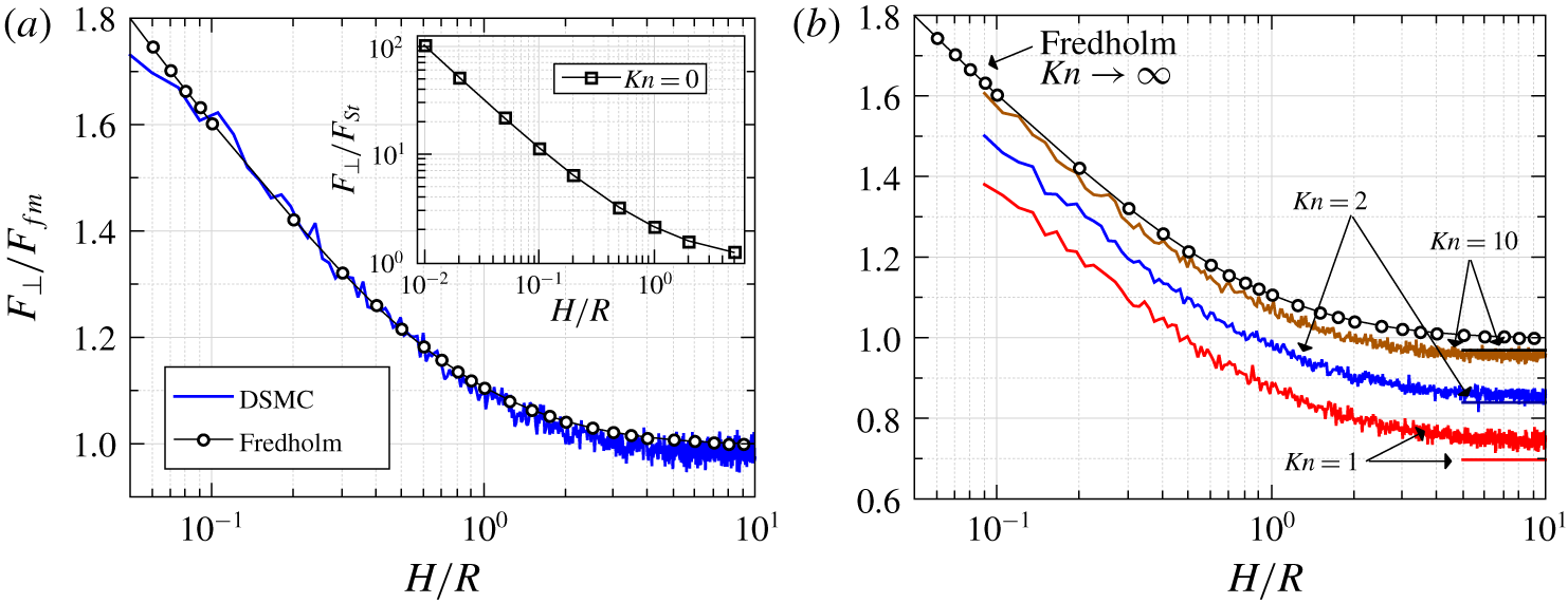
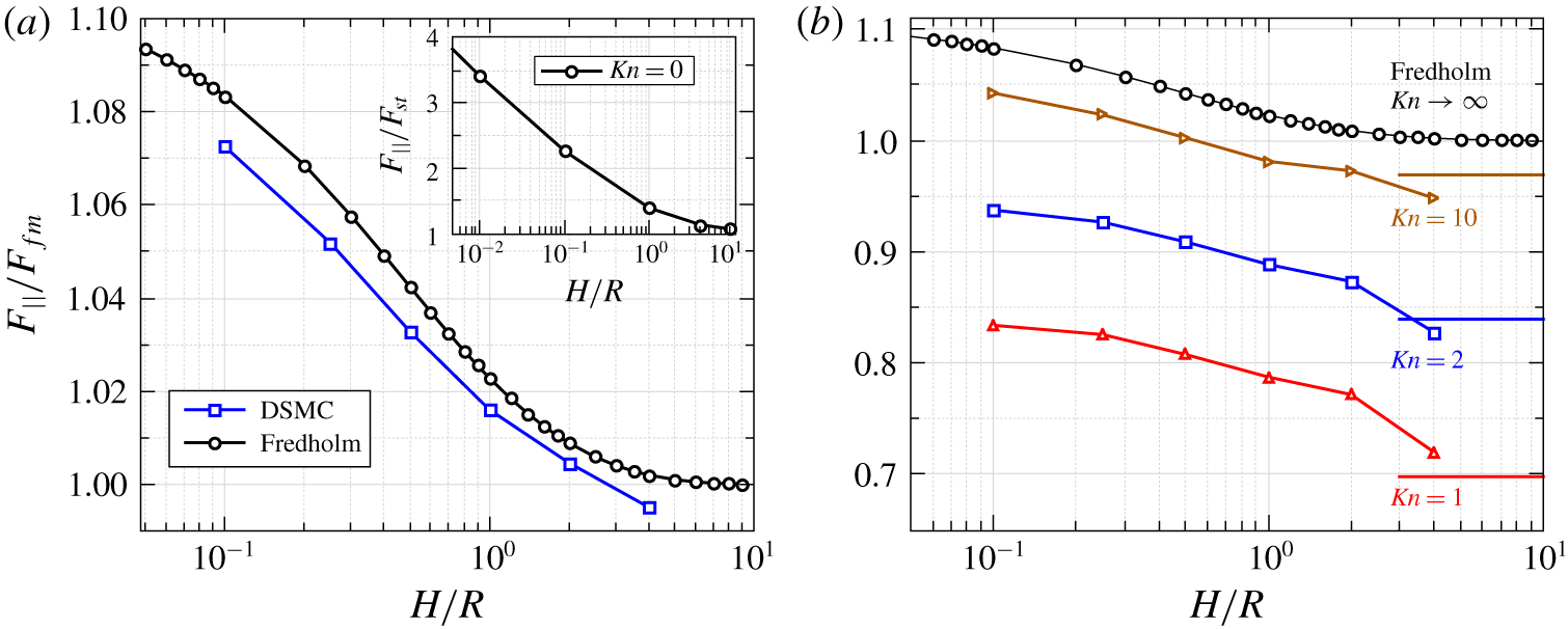
Drag on a sphere moving normal to a plane wall: (a) collisionless regime; (b) at finite  $Kn$. For comparison, the inset in (a) shows the drag in the continuum regime for a no-slip boundary condition normalized by the Stokes drag (Brenner Reference Brenner1961; Maude Reference Maude1961; Goren Reference Goren1973). Horizontal lines in (b) indicate values according to (3.3) for the drag on a sphere moving in an unbounded domain and serve to assess the accuracy of the DSMC calculations.

The normalized drag on a sphere moving normal to a planar wall in the collisionless regime,  $Kn\rightarrow \infty$, is shown in figure 3(a) as a function of the distance to the wall. Note that from the integral equation approach it is evident that due to linearity in
 $Sh$ this increase in drag occurs irrespective of whether the sphere moves towards or away from the plane. For distances above
 $H/R\gtrsim 5$, the difference between the drag obtained based on the integral equations described in section 2 and the drag in an unbounded domain remains below 1 %. In the near-wall region,
 $H/R\lesssim 1$, the wall has a marked influence on the drag, with an 80 % increase for the smallest gap size of
 $H/R=0.05$. For
 $H/R\lesssim 0.1$, the increase is approximately logarithmic. This logarithmic dependence was also found in the slip-flow regime by Hocking (Reference Hocking1973). Sundararajakumar & Koch (Reference Sundararajakumar and Koch1996) argue that in the limit
 $H/R\rightarrow 0$ the dependence becomes
 $\log \log (R/H)$ for free molecular flow. Figure 3(a) also shows corresponding results obtained via the DSMC method, where each data point represents an average of
 $N=870$ individual runs, with the scatter between neighbouring data points indicating the stochastic error inherent in the method. Overall, there is good agreement between the methods used, although there is a tendency of the DSMC method to slightly underestimate the drag by a few per cent for large distances. For comparison, the inset of figure 3(a) shows the drag in the continuum regime for a fluid of viscosity
 $\unicode[STIX]{x1D707}$ and no-slip boundary conditions normalized by the Stokes drag
 $F_{St}=6\unicode[STIX]{x03C0}\unicode[STIX]{x1D707}RU$ (Brenner Reference Brenner1961; Maude Reference Maude1961; Goren Reference Goren1973), highlighting the inverse proportionality of the force on the gap width in this limit. These data indicate the marked difference between the continuum and the free molecular regimes: while within the considered range of
 $H/R$ values, the drag increases by more than one order of magnitude in the continuum regime, it only increases by a factor of 1.8 in the free molecular regime.


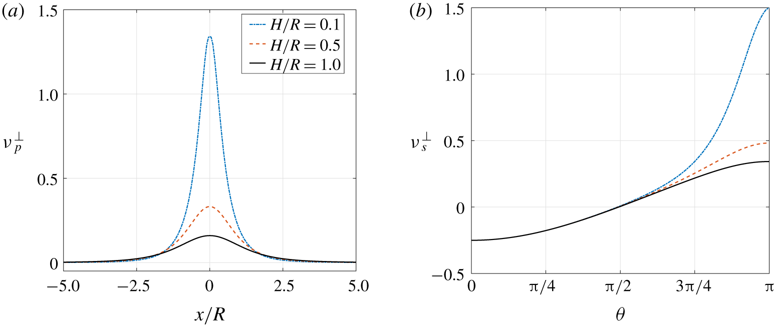
Some exemplary plots of the excess molecular densities  $\unicode[STIX]{x1D708}$ on the plane and the sphere for normal motion corresponding to the results obtained by the Fredholm integral approach, equations (2.11) and (2.12), are shown in figure 4. It is observed that on the plane the molecular density is mainly affected within a region of roughly 2.5 diameters of the sphere for all separations. Correspondingly, on the sphere only the lower spherical cap sees a marked influence of the molecular flux due to the wall. When relating the molecular density to the flux density, we find that for large
 $H/R$ the molecular flux density on the sphere is approximately anti-symmetric between the top,
 $\unicode[STIX]{x1D703}=0$, and the bottom,
 $\unicode[STIX]{x1D703}=\unicode[STIX]{x03C0}$, of the sphere. This nearly corresponds to the molecular density around a moving sphere undisturbed by the wall, as first calculated by Epstein (Reference Epstein1924) and indicated by the first term in (2.11). Note that as mentioned above, the excess molecular flux density is directly proportional to
 $Sh$ due to the linearity of the equations. In particular,
 $\unicode[STIX]{x1D708}$ would change its sign both on the plane and on the sphere in the case of motion away from the plane.
Based on that, the increase in drag on the sphere due to the proximity of the wall can be qualitatively explained as follows. In an unbounded medium, the sphere already experiences an increased molecular flux at its front side and a reduced flux at its back. This flux asymmetry is responsible for the drag force, and is approximately represented by the black solid curve in figure 4(b). The proximity of the wall amplifies the molecular flux at the front side. An approaching sphere locally increases the molecular flux on the plane, and the reflected molecules, in turn, increase the flux at the front side of the sphere. The additional flux corresponds to additional transferred momentum, thereby increasing the drag on the sphere.
In order to assess the influence of molecular collisions on the drag, we show results obtained for  $Kn=1,2$ and 10 in figure 3(b) for a sphere moving normal to the wall. For finite Knudsen numbers an average over
 $N=84$ (for
 $Kn=1$) to 870 (for
 $Kn=10$) independent runs was performed. At
 $Kn=10$ the agreement between DSMC and integral equation results remains good, and for large
 $H/R$ the limiting value for a sphere moving in an unbounded domain is reached. For smaller
 $Kn$ the values for large distances obtained with DSMC lie 5 %–10 % above the values for an unbounded domain predicted from (3.3). A similar observation was already made in the context of figure 2, where discrepancies of a similar magnitude occur and were explained by the finite size of the computational domain. With the magnitude of this error in mind, one can nevertheless state that the normalized drag force on the sphere follows a curve similar to that in the collisionless case, even down to the transition regime. This is plausible, since for the considered
 $Kn$ the flow in the gap increasingly resembles the collisionless situation when
 $H/R$ is reduced.
Drag on a sphere moving parallel to a plane wall: (a) collisionless regime; (b) at finite  $Kn$. The inset in (a) shows the drag in the continuum regime for no-slip boundary conditions normalized by the Stokes drag (Loussaief et al. Reference Loussaief, Pasol and Feuillebois2015). Horizontal lines in (b) indicate values from (3.3) for the drag on a sphere moving in an unbounded domain and serve to asses the accuracy of the DSMC calculation.

Figure 5(a) shows the normalized drag on a sphere moving parallel to a planar wall in the collisionless regime. In this case the presence of the wall only results in a drag increase in excess of 1 % compared to the unbounded situation for  $H/R\lesssim 2$. Note that the influence of the wall on drag for motion parallel to the plane is much smaller than the corresponding influence during normal motion. We remark that in the limit of small
 $Sh$ and large
 $Kn$ considered here, the sphere experiences no lift force, since the excess molecular density
 $\unicode[STIX]{x1D708}_{i}$ on the sphere as well as on the plane is anti-symmetric with respect to the direction of motion. This parallels the result obtained at low
 $Re$ in the continuum regime, where the (dimensional) wall-induced lift is an inertial effect of
 $O(U^{2})$ (Cox & Hsu Reference Cox and Hsu1977; Vasseur & Cox Reference Vasseur and Cox1977; Zeng, Balachandar & Fischer Reference Zeng, Balachandar and Fischer2005). Similarly, in the limit of large
 $Kn$, lift is expected to occur at the same order in
 $U$, with contributions from a rotation of
 $O(U)$ induced by a torque of
 $O(U)$ due to the fore–aft asymmetry in
 $\unicode[STIX]{x1D708}$, which in turn leads to an ‘inverse’ Magnus force (Wang Reference Wang1972) of
 $O(U^{2})$. Due to the smallness of this effect, rotation is neglected in the present study and the exhaustive exploration of lift at finite
 $Kn$ remains an unresolved issue.
For comparison, in figure 5(a) we have again included results obtained with the DSMC method. Note that the DSMC method again predicts a slightly smaller drag than obtained via the Fredholm integral method, although the discrepancy remains within 1 %, providing a fair agreement. The inset shows corresponding results of Loussaief et al. (Reference Loussaief, Pasol and Feuillebois2015) for the drag in the continuum regime with no-slip boundary conditions, showing an increase  ${\sim}\text{log}(R/H)$ for small gap width when the lubrication approximation applies (O’Neill & Stewartson Reference O’Neill and Stewartson1967). Again, there is a very large difference between the continuum and the free molecular regimes in terms of the increase in drag when
 $H/R$ is reduced.
The drag on a sphere in parallel motion at finite  $Kn$ is shown in figure 5(b) as a function of the distance from the wall. Similar to the case of normal motion, the inclusion of molecular collisions only has a small influence at
 $Kn=10$, although the difference from the collisionless result is more apparent. As before, for
 $Kn=1$ and 2 the finite size of the computational domain is expected to influence the result, in particular for large
 $H/R$. In order to assess the magnitude of this influence we have again included the predictions from (3.3) for an unbounded domain. The results again indicate that when collisions are included, the wall has a similar effect on the drag increase with the proximity parameter as in the collisionless case.


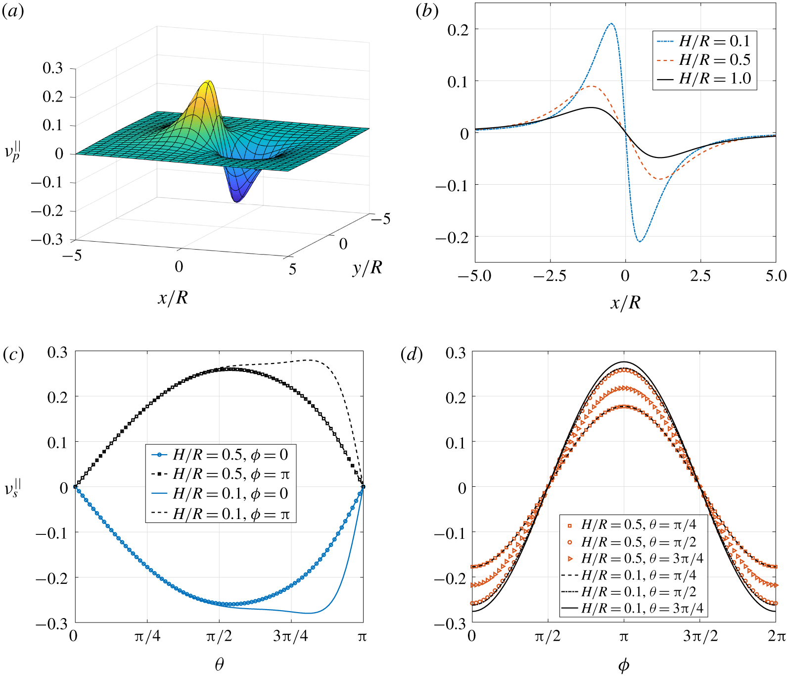
The molecular densities corresponding to the collisionless case are explored in figure 6 for the case of a sphere moving in the negative  $x$ direction. For illustrative purposes we have included a three-dimensional plot of
 $\unicode[STIX]{x1D708}_{p}$ on the planar surface for the case
 $H/R=0.1$ in figure 6(a), while corresponding plots at
 $y=0$ are shown in figure 6(b) for various values of the gap width. Compared to the case of normal motion, it is observed that the moving sphere influences the excess molecular density on the wall on a larger area. The corresponding excess molecular densities
 $\unicode[STIX]{x1D708}_{s}$ on the sphere in its direction of motion,
 $\unicode[STIX]{x1D719}=\unicode[STIX]{x03C0}$, and at the rear,
 $\unicode[STIX]{x1D719}=0$, are shown in figure 6(c), where the influence of the adjacent planar wall is seen on the entire lower hemisphere, and the upper hemisphere remains unaffected. Note the anti-symmetry of the molecular density between the forward and backward directions. In figure 6(d) this anti-symmetry between the forward and backward directions can also be observed for circles of constant
 $\unicode[STIX]{x1D703}$ on the sphere. This is the reason why the lift force on the sphere vanishes in this situation, as mentioned above. In the free molecular flow regime, the increase in drag for a sphere moving parallel to a planar wall can be understood as follows. The molecules reflected from the sphere increase the molecular density (and flux) on the planar wall in the forward direction, while they decrease it in the backward direction. In turn, the molecular flux that the sphere receives from the wall increases (decreases) at the front (at the rear), compared to the molecular flux in an unbounded domain. Therefore, the drag force on the sphere increases due to the proximity of the wall.
5 Conclusions
The hydrodynamic force on a particle moving near a wall has an impact on settling, deposition and Brownian motion. Our investigation quantifies this force for a spherical particle in the collisionless regime at small Strouhal number, using coupled Fredholm integral equations. A much larger increase in force with decreasing gap size between the sphere and the wall is observed for motion normal to the wall compared to parallel motion. The increase in drag force due to the proximity of the wall was explained by the modification of the particle flux density on the planar wall due to the presence of the sphere, which in turn influences the incoming particle flux at the surface of the sphere. Comparison of the free molecular results with DSMC results for various values of  $Kn$ indicates that a similar dependence of the force on the gap size is found in the transition regime. This can be attributed to the flow being essentially a free molecular flow in the gap. These results for the free molecular and the transition regimes represent a marked difference from the continuum regime. In the continuum regime, the increase of the drag force with decreasing gap size is much more pronounced.
Acknowledgements
Financial support by the DFG (Deutsche Forschungsgemeinschaft) under grant numbers HA 2696/41-1 and KL 1105/27-1 is gratefully acknowledged.
Declaration of interests
None.
Appendix A. Drag force on a spherical particle
The integral (2.13) for the force on the sphere can be split into surface integrals
 $$\begin{eqnarray}\boldsymbol{F}_{s}=\int _{S}\left(\frac{\text{d}\boldsymbol{F}_{s}}{\text{d}S}\right)\,\text{d}S=\int _{S}\left[\left(\frac{\text{d}\boldsymbol{F}_{s}}{\text{d}S}\right)^{in}-\left(\frac{\text{d}\boldsymbol{F}_{s}}{\text{d}S}\right)^{out}\right]\,\text{d}S\end{eqnarray}$$
over the differential force contributions due to the incident and reflected molecules:
 $$\begin{eqnarray}\displaystyle \left(\frac{\text{d}\boldsymbol{F}_{s}}{\text{d}S}\right)^{in} & = & \displaystyle n_{\infty }\int _{(\boldsymbol{c}-\boldsymbol{U})\boldsymbol{\cdot }\boldsymbol{n}_{s}<0}m\boldsymbol{c}|(\boldsymbol{c}-\boldsymbol{U})\boldsymbol{\cdot }\boldsymbol{n}_{s}|f_{M}(\boldsymbol{c})\,\text{d}\boldsymbol{c}\nonumber\\ \displaystyle & & \displaystyle +\,\int _{\unicode[STIX]{x1D6FA}_{ps}}m\boldsymbol{c}|(\boldsymbol{c}-\boldsymbol{U})\boldsymbol{\cdot }\boldsymbol{n}_{s}|(n_{p}(\boldsymbol{r}_{p})-n_{\infty })f_{M}(\boldsymbol{c})\,\text{d}\boldsymbol{c},\end{eqnarray}$$
 $$\begin{eqnarray}\left(\frac{\text{d}\boldsymbol{F}_{s}}{\text{d}S}\right)^{out}=\int _{(\boldsymbol{c}-\boldsymbol{U})\boldsymbol{\cdot }\boldsymbol{n}_{s}>0}m\boldsymbol{c}|(\boldsymbol{c}-\boldsymbol{U})\boldsymbol{\cdot }\boldsymbol{n}_{s}|n_{s}(\boldsymbol{r}_{s})f_{M}(\boldsymbol{c}-\boldsymbol{U})\,\text{d}\boldsymbol{c}.\end{eqnarray}$$
Using  $n_{i}(\boldsymbol{r}_{i})=n_{\infty }(1+\unicode[STIX]{x1D708}_{i}(\boldsymbol{r}_{i}))$ in (A 2) and (A 3), one obtains the differential force in the first order of
 $Sh$ as
 $$\begin{eqnarray}\displaystyle & \displaystyle \left(\frac{\text{d}\boldsymbol{F}_{s}}{\text{d}S}\right)^{in}=-kTn_{\infty }\left[\left\{\frac{1}{2}+\sqrt{\frac{m}{2\unicode[STIX]{x03C0}kT}}(\boldsymbol{n}_{s}\boldsymbol{\cdot }\boldsymbol{U})\right\}\boldsymbol{n}_{s}+\frac{3}{4\unicode[STIX]{x03C0}}\int _{\unicode[STIX]{x1D6FA}_{ps}}\boldsymbol{e}_{w}|\boldsymbol{e}_{w}\boldsymbol{\cdot }\boldsymbol{n}_{s}|\unicode[STIX]{x1D708}_{p}(\boldsymbol{r}_{p})\,\text{d}\unicode[STIX]{x1D6FA}_{w}\right], & \displaystyle \nonumber\\ \displaystyle & & \displaystyle\end{eqnarray}$$
 $$\begin{eqnarray}\displaystyle & \displaystyle \left(\frac{\text{d}\boldsymbol{F}_{s}}{\text{d}S}\right)^{out}=kTn_{s}(\boldsymbol{r}_{s})\left\{\frac{1}{2}\boldsymbol{n}_{s}+\sqrt{\frac{m}{2\unicode[STIX]{x03C0}kT}}\boldsymbol{U}\right\}, & \displaystyle\end{eqnarray}$$
with the integration over the solid angle  $\unicode[STIX]{x1D6FA}_{ps}$ as explained after (2.9). Integrating (A 4) and (A 5) with
 $\unicode[STIX]{x1D708}_{s}=\sqrt{\unicode[STIX]{x03C0}}(\boldsymbol{U}\boldsymbol{\cdot }\boldsymbol{n}_{s})/\bar{c}$ and
 $\unicode[STIX]{x1D708}_{p}=0$ according to (A 1) yields Epstein’s result (3.2) for the drag on a sphere, while all contributions on top of that result in the correction due to the presence of the wall.