2 Problem formulation

A leaky dielectric drop (permittivity $\bar{{\it\epsilon}}^{\ast }$ , conductivity $\bar{{\it\sigma}}^{\ast }$ , viscosity $\bar{{\it\mu}}^{\ast }$ ) is suspended in another leaky dielectric liquid (permittivity ${\it\epsilon}^{\ast }$ , conductivity ${\it\sigma}^{\ast }$ , viscosity ${\it\mu}^{\ast }$ ) of an unbounded extent. (Hereafter an asterisk is used to decorate dimensional quantities; the bar decoration is employed for drop-phase variables.) The drop settles due to gravity in a direction specified by the unit vector $\hat{\boldsymbol{\imath }}$ . (When the drop density $\bar{{\it\rho}}^{\ast }$ is larger than the density ${\it\rho}^{\ast }$ of the suspending liquid, this is the gravity direction; if $\bar{{\it\rho}}^{\ast }<{\it\rho}^{\ast }$ $\hat{\boldsymbol{\imath }}$ is in the opposite direction.) In addition, it is exposed to a uniformly applied electric field of magnitude $E^{\ast }$ in that direction. We assume that capillarity is sufficiently strong to maintain an approximately spherical drop, say of radius $a^{\ast }$ . Our interest is in the steady-state solution, and in particular in the settling speed.

The problem is characterised by two velocity scales. The first is the settling velocity in the absence of an applied field, namely

(2.1) $$\begin{eqnarray}{\mathcal{U}}^{\ast }=\frac{1}{3}\frac{M+1}{M+3/2}\frac{|\bar{{\it\rho}}^{\ast }-{\it\rho}^{\ast }|g^{\ast }{a^{\ast }}^{2}}{{\it\mu}^{\ast }},\end{eqnarray}$$

where $M={\it\mu}^{\ast }/\bar{{\it\mu}}^{\ast }$ and $g^{\ast }$ is the acceleration due to gravity. The second is the electrohydrodynamic velocity

(2.2) $$\begin{eqnarray}\frac{{\it\epsilon}^{\ast }a^{\ast }{E^{\ast }}^{2}}{{\it\mu}^{\ast }}.\end{eqnarray}$$

We employ a dimensionless notation, where length variables are normalised by $a^{\ast }$ , velocity variables by ${\mathcal{U}}^{\ast }$ and electric fields by $E^{\ast }$ . The electric potentials (normalised by $a^{\ast }E^{\ast }$ ) in the medium and drop phases are respectively denoted by ${\it\varphi}$ and $\bar{{\it\varphi}}$ ; the corresponding velocity fields are denoted by $\boldsymbol{u}$ and $\bar{\boldsymbol{u}}$ . The dimensionless problem governing these fields depends upon: (i) the ratio of the two velocity scales,

(2.3) $$\begin{eqnarray}W=\frac{{\it\epsilon}^{\ast }a^{\ast }{E^{\ast }}^{2}}{{\it\mu}^{\ast }{\mathcal{U}}^{\ast }};\end{eqnarray}$$

(ii) the material ratios $R=\bar{{\it\sigma}}^{\ast }/{\it\sigma}^{\ast }$ , $S={\it\epsilon}^{\ast }/\bar{{\it\epsilon}}^{\ast }$ and $M={\it\mu}^{\ast }/\bar{{\it\mu}}^{\ast }$ ; and (iii) the electric Reynolds number, provided by the ratio of the charge relaxation time ${\it\epsilon}^{\ast }/{\it\sigma}^{\ast }$ to the convective time $a^{\ast }/{\mathcal{U}}^{\ast }$ :

(2.4) $$\begin{eqnarray}Re=\frac{{\it\epsilon}^{\ast }{\mathcal{U}}^{\ast }}{a^{\ast }{\it\sigma}^{\ast }}.\end{eqnarray}$$

The problem is formulated in a drop-fixed reference system, using spherical coordinates $(r,{\it\theta},{\it\varpi})$ with the radial coordinate $r$ measured from the drop centre and the latitudinal angle ${\it\theta}$ measured from the direction specified by $\hat{\boldsymbol{\imath }}$ . The corresponding unit vectors are denoted $(\hat{\boldsymbol{e}}_{r},\hat{\boldsymbol{e}}_{{\it\theta}},\hat{\boldsymbol{e}}_{{\it\varpi}})$ . Because of axial symmetry, the azimuthal angle ${\it\varpi}$ is degenerate. The velocity fields in the suspending and drops phases are accordingly written $\boldsymbol{u}=\hat{\boldsymbol{e}}_{r}u+\hat{\boldsymbol{e}}_{{\it\theta}}v$ and $\bar{\boldsymbol{u}}=\hat{\boldsymbol{e}}_{r}\bar{u}+\hat{\boldsymbol{e}}_{{\it\theta}}\bar{v}$ .

The electrostatic problem consists of: (i) Laplace’s equation outside and inside the drop; (ii) electric potential continuity

(2.5) $$\begin{eqnarray}{\it\varphi}=\bar{{\it\varphi}}\quad \text{at }r=1;\end{eqnarray}$$

(iii) regularity inside the drop; and (iv) the far-field condition

(2.6) $$\begin{eqnarray}{\it\varphi}\sim -r\cos {\it\theta}\quad \text{as }r\rightarrow \infty ,\end{eqnarray}$$

corresponding to a unit field in the $\hat{\boldsymbol{\imath }}$ -direction. In addition, it also consists of the charging condition

(2.7) $$\begin{eqnarray}\frac{\partial {\it\varphi}}{\partial r}-R\frac{\partial \bar{{\it\varphi}}}{\partial r}=\frac{Re}{\sin {\it\theta}}\frac{\partial }{\partial {\it\theta}}(qv\sin {\it\theta})\quad \text{at }r=1,\end{eqnarray}$$

wherein

(2.8) $$\begin{eqnarray}q=S^{-1}\frac{\partial \bar{{\it\varphi}}}{\partial r}-\frac{\partial {\it\varphi}}{\partial r}\end{eqnarray}$$

is the surface-charge density (normalised by ${\it\epsilon}^{\ast }E^{\ast }$ ).

The SCC term in the right-hand side of (2.7) introduces a coupling to the velocity field. The flow is governed by the continuity and Stokes equations in the two phases. At the drop boundary $r=1$ it satisfies the kinematic condition of vanishing radial velocities,

(2.9) $$\begin{eqnarray}u=\bar{u}=0,\end{eqnarray}$$

the dynamic condition of tangential velocity continuity,

(2.10) $$\begin{eqnarray}v=\bar{v}\end{eqnarray}$$

(already tacitly used in (2.7)) and the shear-stress condition, balancing hydrodynamic viscous stresses with electric shear stresses,

(2.11) $$\begin{eqnarray}\hat{\boldsymbol{e}}_{r}\boldsymbol{\cdot }(\unicode[STIX]{x1D64E}-\bar{\unicode[STIX]{x1D64E}})\boldsymbol{\cdot }\hat{\boldsymbol{e}}_{{\it\theta}}=Wq\frac{\partial {\it\varphi}}{\partial {\it\theta}},\end{eqnarray}$$

wherein $\unicode[STIX]{x1D64E}$ and $\bar{\unicode[STIX]{x1D64E}}$ respectively denote the hydrodynamic stresses at the two phases. At large distances the velocity approaches a uniform velocity,

(2.12) $$\begin{eqnarray}\boldsymbol{u}\rightarrow -U\hat{\boldsymbol{\imath }}\quad \text{as }r\rightarrow \infty .\end{eqnarray}$$

The settling velocity $U$ is determined by the condition that the sum of external and hydrodynamic forces on the drop vanishes, resulting in a nonlinear ‘mobility’ problem. In general, then, the settling velocity is a function of both $W$ and $Re$ , as well as the ratios $R$ , $S$ and $M$ .

3 General properties

Due to the SCC term in (2.7) the problem is inherently nonlinear. No closed form analytic solution is accordingly expected. (Note that no analytic solution is known even in the absence of gravity.) Nonetheless, there are three general observations which can be made immediately (cf. Yariv & Frankel Reference Yariv and Frankel2016).

The first is that the net surface charge must vanish,

(3.1) $$\begin{eqnarray}\oint _{r=1}q\,\text{d}A=0\end{eqnarray}$$

(wherein the areal element $\text{d}A$ is normalised by ${a^{\ast }}^{2}$ ). Indeed, by Gauss law a net interfacial charge must be accompanied by a net electric flux through any closed surface which encloses the drop. Because of the Ohmic nature of the leaky dielectric liquid, such a flux would be equivalent to a net electric current emanating from the drop, in contradiction to the assumed steady state. Mathematically, Laplace’s equation inside the drop implies that the integral of $\partial \bar{{\it\varphi}}/\partial r$ over the unit sphere $r=1$ must vanish. The charging condition (2.7) then necessitates the same for $\partial {\it\varphi}/\partial r$ . Using (2.8), (3.1) readily follows. The absence of charge in conjunction with Laplace’s equation and the approach (2.6) to a uniform field implies that the drop does not experience any electric force (Rivette & Baygents Reference Rivette and Baygents1996; Yariv Reference Yariv2006). It follows that the external force on the drop is only due to gravity.

The second observation is that in the absence of such an external force, the problem retains the familiar symmetry about the mid-plane ${\it\theta}={\rm\pi}/2$ , implicit in the original problem of Taylor (Reference Taylor1966). Thus, under the reflection ${\it\theta}\rightarrow {\rm\pi}-{\it\theta}$ the pertinent fields transform as

(3.2a-d ) $$\begin{eqnarray}({\it\varphi},\bar{{\it\varphi}})\rightarrow (-{\it\varphi},-\bar{{\it\varphi}}),\quad q\rightarrow -q,\quad (u,\bar{u})\rightarrow (u,\bar{u}),\quad (v,\bar{v})\rightarrow (-v,-\bar{v}).\end{eqnarray}$$

Indeed, it may be readily verified that this symmetry in unaffected by nonlinear SCC term. (We do not consider here large electric Reynolds numbers, where this nonlinear term may result in a spontaneous symmetry breaking, see Yariv & Frankel Reference Yariv and Frankel2016.) It follows that the drop does not move, $U=0$ . (This, of course, is the motivation for incorporating gravity effects in the first place.)

The third observation is that nonlinearities are introduced into the problem only through the boundary conditions, namely the charging condition governing the electrostatics and the shear-stress condition governing the flow. Since the governing differential equations are linear, the electric potentials and fluid velocities may be represented via appropriate eigenfunction expansions. In particular, the harmonic electric potential outside the drop may be written as a sum of spherical harmonics. Thus, using (2.6) and the axial symmetry we write

(3.3) $$\begin{eqnarray}{\it\varphi}=-rP_{1}({\it\eta})+\mathop{\sum }_{n=1}^{\infty }A_{n}\frac{P_{n}({\it\eta})}{r^{n+1}},\end{eqnarray}$$

wherein ${\it\eta}=\cos {\it\theta}$ and $P_{n}({\it\eta})$ are the Legendre polynomials of degree $n$ . (Note the absence of a monopole term, in accordance with (3.1).) Because of (2.5) and the requirement of regularity within the drop, the potential there is

(3.4) $$\begin{eqnarray}\bar{{\it\varphi}}=-rP_{1}({\it\eta})+\mathop{\sum }_{n=1}^{\infty }A_{n}r^{n}P_{n}({\it\eta}).\end{eqnarray}$$

In the absence of SCC (i.e. for $Re=0$ ) the solution of the electrostatic problem is trivial, involving only the Legendre polynomial of the first degree (Melcher & Taylor Reference Melcher and Taylor1969)

(3.5a,b ) $$\begin{eqnarray}{\it\varphi}=-\!\left(r+\frac{1-R}{2+R}r^{-2}\right)\cos {\it\theta},\quad \bar{{\it\varphi}}=-\frac{3}{2+R}r\cos {\it\theta}.\end{eqnarray}$$

In the presence of SCC, expansions (3.3)–(3.4) generally consist of an infinite number of terms.

4 Weak fields

We focus here upon the case where the applied field is weak, in the sense that the electrohydrodynamic scale (2.2) is small compared with the characteristic settling velocity ${\mathcal{U}}^{\ast }$ :

(4.1) $$\begin{eqnarray}W\ll 1.\end{eqnarray}$$

The leading-order flow field is therefore that associated with drop settling in the absence of any electrohydrodynamic effects due to a prescribed external force. Since this field may be considered as known, the SCC term in (2.7) becomes linear in the field, as is then the entire leading-order electrostatic problem.

Given definition (2.1) of the velocity scale, the drop settles at leading order with a unit speed (i.e. $U=1$ in (2.12)). Within approximation (4.1) the leading-order ‘electrohydrodynamic’ correction to the velocity field is animated by the electrical shear stresses associated with the leading-order electric field distribution. Since the hydrodynamic force associated with the leading-order flow already balances the external force due to gravity, the electrohydrodynamic correction must result in a nil hydrodynamic force. Defining

(4.2) $$\begin{eqnarray}U=1+W\tilde{U} +\cdots \,.\end{eqnarray}$$

The correction $\tilde{U}$ to the settling velocity is set by this force-free condition. Our goal is the calculation of this correction. Note that $\tilde{U}$ represents a normalization by the electrohydrodynamic velocity scale (2.2).

The $O(W)$ electrohydrodynamic flow is governed by the continuity and Stokes equations, impermeability and velocity continuity conditions at $r=1$ (cf. (2.9)–(2.10)), far-field approach to $-\tilde{U} \hat{\boldsymbol{\imath }}$ (cf. (2.12)), and the force-free condition. It is driven by an inhomogeneous shear-stress condition (see (2.11)) associated with the distribution $-q(\partial {\it\varphi}/\partial {\it\theta})_{r=1}$ of electric shear stresses. (Hereafter $q$ and ${\it\varphi}$ refer to the respective leading-order quantities.)

Our interest lies in the electrohydrodynamic correction to the settling speed, rather than the detailed flow field associated with it. Using the reciprocal theorem of Stokes flow (Happel & Brenner Reference Happel and Brenner1965), this correction may be obtained as a linear functional of the electric-stress distribution. Thus, making use of the general result obtained by Nadim, Haj-Hariri & Borhan (Reference Nadim, Haj-Hariri and Borhan1990) we obtain here

(4.3) $$\begin{eqnarray}\tilde{U} =\frac{1}{8{\rm\pi}}\frac{M}{M+3/2}\hat{\boldsymbol{\imath }}\boldsymbol{\cdot }\oint _{r=1}\text{d}A\,\hat{\boldsymbol{e}}_{{\it\theta}}q\frac{\partial {\it\varphi}}{\partial {\it\theta}}.\end{eqnarray}$$

Upon substituting (2.8) and reverting to ${\it\eta}$ as the integration variable,

(4.4) $$\begin{eqnarray}\tilde{U} =-\frac{1}{4}\frac{M}{M+3/2}\int _{-1}^{1}(1-{\it\eta}^{2})\left.\left(\frac{\partial {\it\varphi}}{\partial r}-S^{-1}\frac{\partial \bar{{\it\varphi}}}{\partial r}\right)\frac{\partial {\it\varphi}}{\partial {\it\eta}}\right|_{r=1}\,\text{d}{\it\eta}.\end{eqnarray}$$

Substituting (3.3)–(3.4) and making use of (5.4) and (5.6) in conjunction with the orthogonality of the Legendre polynomials eventually furnishes the desirable formula

(4.5) $$\begin{eqnarray}\displaystyle \frac{M+3/2}{M}\tilde{U} & = & \displaystyle \frac{6-S^{-1}}{15}A_{2}+\mathop{\sum }_{n=1}^{\infty }\frac{n+1+nS^{-1}}{2(2n+1)}A_{n}\nonumber\\ \displaystyle & & \displaystyle \times \left[\frac{(n+1)(n+2)}{2n+3}A_{n+1}-\frac{n(n-1)}{2n-1}A_{n-1}\right].\end{eqnarray}$$

It is worth emphasising that, in the limit (4.1), the electric potential satisfies a linear problem while the drop velocity is quadratic in that potential. The assumption, made in the problem formulation, that the applied field points in the settling direction $\hat{\boldsymbol{\imath }}$ (parallel to gravity for $\bar{{\it\rho}}^{\ast }>{\it\rho}^{\ast }$ , anti-parallel to it for $\bar{{\it\rho}}^{\ast }<{\it\rho}^{\ast }$ ) is accordingly non-restrictive. Indeed, an applied field in the opposite direction would simply reverse the electric field distribution, resulting in an identical value of $\tilde{U}$ .

5 Electrostatic problem

In the drop-fixed reference system, where at large $r$ the velocity tends to $-\hat{\boldsymbol{\imath }}$ , the interfacial velocity is (Happel & Brenner Reference Happel and Brenner1965)

(5.1) $$\begin{eqnarray}v=\frac{M}{2(1+M)}\sin {\it\theta}.\end{eqnarray}$$

We accordingly consider the electrostatic problem resulting from substitution of the leading-order distribution (5.1) into the SCC term. Thus, substitution of (3.3)–(3.4) and (5.1) into the respective left- and right-hand sides of (2.7) followed by integration readily yields

(5.2) $$\begin{eqnarray}\int _{-1}^{{\it\eta}}\left[(1-R)P_{1}(t)+\mathop{\sum }_{n=1}^{\infty }(n+1+nR)A_{n}P_{n}(t)\right]\,\text{d}t=\frac{\mathscr{R}}{2}(1-{\it\eta}^{2})q,\end{eqnarray}$$

wherein the electric Reynolds number and viscosity ratio appear through the single group

(5.3) $$\begin{eqnarray}\mathscr{R}=\frac{M}{1+M}Re.\end{eqnarray}$$

Use of the following form of the Legendre equation

(5.4) $$\begin{eqnarray}n(n+1)\int _{-1}^{{\it\eta}}P_{n}(t)\,\text{d}t=-(1-{\it\eta}^{2})P_{n}^{\prime }({\it\eta})\end{eqnarray}$$

(wherein the prime denote differentiation) and substitution of (2.8) gives

(5.5) $$\begin{eqnarray}\frac{1-R}{2}P_{1}^{\prime }({\it\eta})+\mathop{\sum }_{n=1}^{\infty }\frac{n+1+nR}{n(n+1)}A_{n}P_{n}^{\prime }({\it\eta})=\frac{\mathscr{R}}{2}\left(\frac{\partial {\it\varphi}}{\partial r}-S^{-1}\frac{\partial \bar{{\it\varphi}}}{\partial r}\right).\end{eqnarray}$$

Substitution of (3.3)–(3.4) into the right-hand side and making use of the identity

(5.6) $$\begin{eqnarray}P_{n}({\it\eta})=\frac{P_{n+1}^{\prime }({\it\eta})-P_{n-1}^{\prime }({\it\eta})}{2n+1},\end{eqnarray}$$

in conjunction with the orthogonality of the derivatives of the Legendre polynomials (with respect to $1-{\it\eta}^{2}$ ), yields

(5.7) $$\begin{eqnarray}\displaystyle & & \displaystyle A_{n}+\frac{n(n+1)\mathscr{R}}{2(n+1+nR)}\left\{\frac{n+(n-1)S^{-1}}{2n-1}A_{n-1}-\frac{n+2+(n+1)S^{-1}}{2n+3}A_{n+1}\right\}\nonumber\\ \displaystyle & & \displaystyle \quad =\left\{\begin{array}{@{}ll@{}}\displaystyle \frac{R-1}{R+2}, & n=1,\\ \displaystyle \frac{S^{-1}-1}{3+2R}\mathscr{R}, & n=2,\\ 0, & n>2,\end{array}\right.\end{eqnarray}$$

where we take $A_{0}=0$ . We have therefore obtained an infinite tridiagonal system governing the coefficients $\{A_{n}\}_{n=1}^{\infty }$ .

6 Small $Re$

For small $Re$ an approximate solution is readily obtained by linearising about (3.5), where all coefficients except $A_{1}$ vanish. Thus, at $O(Re)$ we find a non-zero $A_{2}$ . The $O(Re)$ excess velocity (4.5) is proportional to the product of these two coefficients, giving

(6.1) $$\begin{eqnarray}\tilde{U} =-\frac{18M^{2}(RS-1)(RS+S-1/3)}{5(1+M)(3+2M)(2+R)^{2}(3+2R)S^{2}}Re,\end{eqnarray}$$

in agreement with equation (34) of Xu & Homsy (Reference Xu and Homsy2006). For $RS>1$ $\tilde{U}$ is negative, while for $1/3<RS<1$ it is positive. For $RS<1/3$ $\tilde{U}$ is positive if $RS>1/3-S$ (which is always the case for $S>1/3$ ) and negative otherwise (in which case $S<1/3$ ). In the limit of a gas bubble, where $R=0$ and $M=\infty$ ,

(6.2) $$\begin{eqnarray}\tilde{U} =\frac{3(S-1/3)}{20S^{2}}Re.\end{eqnarray}$$

For a gas bubble $\bar{{\it\epsilon}}^{\ast }$ is approximately that of vacuum meaning that $S\geqslant 1$ ; $\tilde{U}$ is therefore positive.

Since the present approximation scheme, where $Re$ is arbitrary and $W\ll 1$ , is ‘orthogonal’ to that made by Xu & Homsy (Reference Xu and Homsy2006), where $W$ is arbitrary and $Re\ll 1$ , the agreement with Xu & Homsy (Reference Xu and Homsy2006) may appear surprising. To understand it, it is useful to consider carefully the small- $Re$ limit of Xu & Homsy, keeping in mind the physical origin of the pertinent terms. The leading-order flow in that limit is a superposition of two components. The first, associated with ‘pure settling’, is independent of the electric field; it is therefore identical to the leading-order flow in the present approximation scheme. The second ‘purely electrohydrodynamic’ component, is proportional to $W$ (i.e. to the square of the applied field magnitude). Since the leading-order surface-charge density is proportional to the applied field, the SCC term associated with the leading-order product of tangential velocity surface-charge density also decomposes into two parts, one proportional to the applied field, the other to its cube. The second part, however, simply represents SCC in the absence of gravity; as such, it does not affect the drop velocity (see (3.2) et seq.). The perturbation to the electric potential (and to the surface charge) due to SCC is accordingly proportional to the field. The resulting modification to the drop velocity is driven by quadratic interaction of that perturbation with the leading-order electric potential, which is also proportional to the field. The velocity modification is accordingly proportional to the field square, or, in dimensionless terms, to $W$ – just as though a perturbation in $W$ was carried out from the outset.

7 Finite $Re$

Consider now the difference equation (5.7) for arbitrary $Re$ . While no analytic solution appears generally possible, (We have managed to obtain closed form analytic solutions for the case $R=0$ and $S=1$ when $\mathscr{R}=1,1/2,1/3,\ldots .$ ) useful information may be extracted by considering the large- $n$ asymptotic limit, where this equation becomes

(7.1) $$\begin{eqnarray}A_{n}=\frac{n}{2{\it\alpha}}[1+O(n^{-1})](A_{n+1}-A_{n-1}),\end{eqnarray}$$

in which

(7.2) $$\begin{eqnarray}{\it\alpha}=\frac{2S(1+R)}{\mathscr{R}(1+S)}.\end{eqnarray}$$

This homogenous second-order equation possesses two solutions. To ensure convergence of the original series (3.3), only the solution that decays at large $n$ is admissible. It may then be verified that

(7.3) $$\begin{eqnarray}A_{n}\sim \text{const.}\times \frac{(-)^{n}}{n^{{\it\alpha}}}\quad \text{as }n\rightarrow \infty ,\end{eqnarray}$$

wherein the asymptotic correction is of relative order $n^{-1}$ . Considering the summation in (4.5), the series converges if and only if ${\it\alpha}>1/2$ , i.e. when

(7.4) $$\begin{eqnarray}Re<\frac{4S(1+R)(1+M)}{M(1+S)}.\end{eqnarray}$$

For an arbitrary $Re$ satisfying (7.4) the system (5.7) is solved using controlled truncation, where the infinite equation set is approximated by a finite set of $N$ equations. Thus, making use of the leading-order approximation (7.3) we replace $A_{N+1}$ in the $N$ th equation by $-A_{N}/(1+1/N)^{{\it\alpha}}$ . In calculating the series (4.5) we estimate the ‘tail’ contribution from $\{A_{n}\}_{n=N+1}^{\infty }$ using the above leading-order approximation. This provides a rapid convergence scheme even when $Re$ is close to the critical value specified by (7.4).

Figure 1.

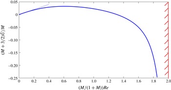
Rescaled velocity $(M+3/2)\tilde{U} /M$ as a function of $\mathscr{R}$ for $R=0$ and $S=1$ . The thin line depicts the corresponding small- $Re$ approximation (7.5) of slope $1/10$ . The critical value $\mathscr{R}=2$ is indicated.

Note that the value of $M$ enters (5.7) only through the rescaled electric Reynolds number $\mathscr{R}$ . Similarly, (4.5) provides the rescaled velocity $(M+3/2)\tilde{U} /M$ as a series which is independent of $M$ . It follows that we may obtain results valid for all $M$ using a single calculation. Such a calculation is illustrated in figure 1 showing the rescaled velocity as a function of $\mathscr{R}$ for $R=0$ and $S=1$ , where the critical value of $\mathscr{R}$ is $2$ . Also shown is the corresponding small- $Re$ approximation,

(7.5) $$\begin{eqnarray}\tilde{U} =\frac{M^{2}}{5(1+M)(3+2M)}Re,\end{eqnarray}$$

obtained from (6.1). Note the non-monotonic variation with the electric Reynolds number and, in particular, the transition from a positive to negative $\tilde{U}$ .

8 Experimental relevance

The key assumption of the present approximation scheme is that the ratio $W$ of electric and gravity forces is small while the electric Reynolds number is $O(1)$ . It is also assumed that the drop is approximately spherical and that inertia plays a negligible role. We here illustrate that these assumptions are indeed compatible with realistic experimental systems.

We first note that, while $W$ is proportional to the square of the applied field magnitude $E^{\ast }$ , the electric Reynolds number is independent of it. Thus, provided the applied field is sufficiently weak $W$ can always be made sufficiently small without affecting $Re$ . It therefore remains to verify that $Re$ can indeed reach $O(1)$ values while the viscous Reynolds number remains small.

Recall also that, in the absence of an electric field, a settling drop does not deform in the Stokes flow regime, regardless of the value of the capillary number (Levich Reference Levich1962). Drop deformation thus occurs at leading order due to the $O(W)$ stresses animated by the electric field, and accordingly scales as the product of $W$ and the appropriate capillary number $Ca$ . The assumption of a nearly spherical drop is trivially satisfied even for $O(1)$ capillary numbers.

An even stricter demand from that of approximate sphericity is that the SCC-induced $O(W)$ perturbation to the settling speed, calculated herein, dominates the comparable perturbation due to deviation from sphericity. This ensures that the velocity perturbation calculated in the present approximation scheme could be directly compared to that measured experimentally. Since drop deformation results in an $O(W\,Ca)$ correction to the settling speed, this requires that the capillary number itself be small.

Plugging the velocity scale (2.1) into (2.4) we see that the electric Reynolds number is of order

(8.1) $$\begin{eqnarray}\frac{{\it\epsilon}^{\ast }|\bar{{\it\rho}}^{\ast }-{\it\rho}^{\ast }|g^{\ast }a^{\ast }}{{\it\mu}^{\ast }{\it\sigma}^{\ast }},\end{eqnarray}$$

linear in drop size. The capillary number $Ca$ is ${\it\mu}^{\ast }{\mathcal{U}}^{\ast }/{\it\gamma}^{\ast }$ , wherein ${\it\gamma}^{\ast }$ the interfacial tension coefficient. Since the velocity scale (2.1) is set by gravity, it coincides here with the Bond number, namely

(8.2) $$\begin{eqnarray}Ca=\frac{|\bar{{\it\rho}}^{\ast }-{\it\rho}^{\ast }|g^{\ast }{a^{\ast }}^{2}}{{\it\gamma}^{\ast }},\end{eqnarray}$$

and scales as the square of drop size. The viscous Reynolds number is

(8.3) $$\begin{eqnarray}\frac{{\it\rho}^{\ast }|\bar{{\it\rho}}^{\ast }-{\it\rho}^{\ast }|g^{\ast }{a^{\ast }}^{3}}{{{\it\mu}^{\ast }}^{2}},\end{eqnarray}$$

proportional to the cube of drop size.

To estimate the above three numbers consider the experiments of Xu & Homsy (Reference Xu and Homsy2006), where a millimetric size phenylmethylsiloxane-dimethylsiloxane (PMM) drop was suspended in castor oil. This choice of liquids was motivated by the large density difference, $\bar{{\it\rho}}^{\ast }-{\it\rho}^{\ast }\approx 40~\text{kg}~\text{m}^{-3}$ , which allows for a significant settling speed. For castor oil Xu & Homsy (Reference Xu and Homsy2006) provide the values ${\it\rho}^{\ast }\approx 960~\text{kg}~\text{m}^{-3}$ and ${\it\mu}^{\ast }\approx 1.4~\text{kg}~\text{m}^{-1}~\text{s}^{-1}$ , as well as a dielectric constant of about 5. There is a significant uncertainty regarding the value of castor oil conductivity. We here use the estimate ${\it\sigma}^{\ast }\approx 10^{-11}~\text{S}~\text{m}^{-1}$ provided by Vizika & Saville (Reference Vizika and Saville1992). (In their comparison with theoretical predictions, Xu & Homsy postulate the even smaller value $2.4\times 10^{-12}~\text{S}~\text{m}^{-1}$ .)

Taking $a^{\ast }=10^{-3}~\text{m}$ and making use of the above mentioned values we find from (8.1) that the electric Reynolds number is about unity. The Bond number, estimated using (8.2) and the value ${\it\gamma}^{\ast }\approx 5\times 10^{-3}~\text{N}~\text{m}^{-1}$ provided by Xu & Homsy (Reference Xu and Homsy2006), is approximately $0.1$ . The Reynolds number (8.3) is of order $10^{-4}$ . These values support our approximation scheme. If silicone oil is used instead of castor oil as the suspending fluid, the conductivity reduces to about $10^{-12}~\text{S}~\text{m}^{-1}$ . Since the density difference $\bar{{\it\rho}}^{\ast }-{\it\rho}^{\ast }\approx 30~\text{kg}~\text{m}^{-3}$ is comparable to that above, this choice can lead to even larger values of $Re$ .

9 Concluding remarks

We have considered the electrohydrodynamic problem of drop settling in the presence of an electric field, accounting for SCC. By focusing upon weak fields we have obtained a linear problem governing the electric potential, valid for all values of $Re$ . Once the electrostatic problem is solved, the excess drop velocity (relative to that in the absence of a field) may be obtained as a linear functional of the associated electric shear stress. Our approach provides a different perspective from that of Xu & Homsy (Reference Xu and Homsy2006), who considered small electric Reynolds numbers but fields which are not weak. Remarkably, it turns out that despite the present weak-field assumption our scheme reproduces at small $Re$ the approximation obtained by Xu & Homsy (Reference Xu and Homsy2006).

The linear electrostatic problem has been reduced to a difference equation governing the respective coefficients in a spherical harmonics expansion of the electric potential. Using this expansion, the integral formula for the drop speed reduces to a single series, quadratic in these coefficients. Inspection reveals a singularity at a critical electric Reynolds number whose value is explicitly obtained in terms of the material ratios $R$ , $S$ and $M$ . For electric Reynolds numbers smaller from the critical values we find a non-monotonic variation of drop speed with the applied field-magnitude. In particular, we observe a transition from velocity enhancement at small $Re$ to velocity decrement at larger $Re$ values.

The finite- $Re$ singularity discovered herein and the trends observed in figure 1 illustrate the limitation of the small- $Re$ approximation and motivate the respective nonlinear analysis of the problem for arbitrary values of $W$ and $Re$ . Since nonlinearity enters the flow problem only through the shear-stress condition (2.11), the velocity field may be conveniently expanded using the appropriate eigenfunction of the Stokes equations in spherical coordinates (Happel & Brenner Reference Happel and Brenner1965). Conditions (2.7) and (2.11) would then involve both the coefficients of such an expansion as well as those of expansion (3.3). This nonlinear analysis, and in particular the behaviour near the critical electric Reynolds number identified herein, is suggested as an open problem. An even more challenging problem arises when the electric field in not aligned with the direction of gravity. This problem was recently analysed assuming a small electric Reynolds number (Bandopadhyay et al. Reference Bandopadhyay, Mandal, Kishore and Chakraborty2016).

In both the pioneering paper of Xu & Homsy (Reference Xu and Homsy2006) and the present contribution the quantity of interest is the modification to the settling velocity due to electric field application. This concept can be easily generalised by considering the effect of ambient flow rather than gravity. In the absence of an electric field the drop is entrained by the flow, moving with a velocity given by Faxén’s law. In the presence of an external electric field, the SCC-induced electric stresses result in a different drop velocity. The respective velocity modification may be calculated in principle using an analogue of the present weak-field scheme, where appropriate use of the reciprocal theorem would provide it as a linear functional of the electric shear stresses. Since the electric stresses in the weak-field scheme are quadratic in the leading-order electric potential distribution, and given the clear nonlinear dependence of that distribution upon $Re$ (see (2.7)), it is evident that the velocity modification is nonlinear in the magnitude of the ambient flow. The well-known symmetry arguments of Stokes flow (Jeffrey Reference Jeffrey and Torry1996) are then inapplicable.

The simplest non-trivial scenario may be that of a drop in a simple shear flow (Vlahovska Reference Vlahovska2011). In the absence of an electric field, the symmetry arguments of Stokes flow preclude drop migration across the streamlines; in fact, the drop simply moves with the velocity of the ambient streamline passing through its centre (Kim & Karrila Reference Kim and Karrila2005). In the presence of an electric field, however, the breakdown of these arguments imply the possibility of migration across streamlines. This may be the case even when the field is applied in the flow direction, because of the asymmetry introduced by the shear direction. (This asymmetry enters the problem through the counterpart of the interfacial velocity profile (5.1) which, for a drop suspended in a shear flow, lacks axial symmetry.) There is some conceptual similarity of this field-induced nonlinear mechanism for cross-streamline migration and that due to Marangoni stresses (Pak, Feng & Stone Reference Pak, Feng and Stone2014), where nonlinearity stems from solute advection.