2.1 Basic concepts and theoretical background

Central to RST is the concept of indiscernibility. Let I = (U,A) be an information system, where U is a non-empty set of finite objects (the universe of discourse) and A is a non-empty finite set of attributes such that for every . V_a is the set of values that attribute a may take. For any , there is an associated equivalence relation IND(P):

(1)

The partition of U, generated by IND(P), is denoted by U/IND(P) and can be defined as follows:

(2)

where,

(3)

and,

(4)

If (x, y)∈IND(P), then x and y are indiscernible by attributes from P. The equivalence classes of the P-indiscernibility relation are denoted by [x]_P.

Let can be approximated using only the information contained within P by constructing the P-lower and P-upper approximations of X:

(5)

(6)

Let P and Q be equivalence relations over U; then the positive, negative, and boundary regions are defined by:

(7)

(8)

(9)

The positive region contains all objects of U that can be classified to classes of using the information in attribute P. The boundary region, BND_P(Q), is the set of objects that can possibly, but not certainly, be classified in this way. The negative region, NEG_P(Q), is the set of objects that cannot be classified to classes of .

2.1.1 Example

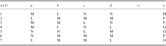
To illustrate the above concepts, a short example in the form of an information system is employed. There are four conditional attributes: a, b, c, and d, and a single decisional attribute, e.

Using the indiscernibilty concept, the data in Table 1 can be partitioned according to the outcome. V_a is the set of values that attribute a may take (in this case L, M, or N). In a decision system, where C denotes the set of condition attributes and D denotes the set of decision attribute(s). There are associated equivalence relations with any :

(10)

Table 1

Example data set

For the data in Table 1—the partition of U by the attribute a would be:

(11)

And for the same table using attributes {b,c}

(12)

This relates to the partition or grouping of the attributes where: a = L (objects 1, 3, and 4), a = M (objects 2 and 7), and a = N (objects 5 and 6). The equivalence classes of the P-indiscernibility relation are denoted by [x]_P. Let . X can be approximated using only the information within P by formulating lower and upper approximations of X as described previously.

2.2 Rough set dependency and other measures

An important aspect of data analysis is the discovery of dependencies between attributes. From an intuitive point of view, an attribute or a set of attributes Q can depend on a set of attributes P, denoted by P Q if all values of attribute(s) in Q are determined uniquely by values of attribute(s) from P. Another way of describing this is that Q depends totally on P if a functional dependency exists between the values of Q and P.

Referring to the example in the previous section, the rough set dependency of the set of attributes Q on a set of attributes P can be seen. For , it can be said that Q depends on P to a degree k (where k∈ [0,1]) denoted by P _k Q if:

(13)

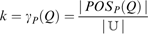
where

(14)

is the positive region of the partition of the universe with respect to P (i.e. the set of all elements that can be classified uniquely into sets of the partition in terms of P).

If k = 1, Q is completely dependent on P, if k < 1 Q is partially dependent (to a degree—k) on P and obviously, if k = 0, Q is completely non-dependent on P. Calculation of the relevant dependencies of each attribute (or group of attributes) allows the significance of that attribute (or group) to be realized.

Taking the data from the example decision table (Table 1), the degree of dependency of attribute {e} upon the attributes {b, c} is:

For the application of feature selection, the minimization of attributes can be realized through the comparison of equivalence relations generated by sets of attributes ({b, c} for the purpose of the previous example). Attributes are removed such that the minimized set provides an equivalent predictive characteristic as the initial decision feature. This minimized set is termed a reduct and can be defined as a subset R of the conditional attribute set C such that .

Other measures have also been used to discover rough set reducts. For instance, in Han et al. (2004), a feature selection method which is based on an alternative dependency measure is presented. This technique was proposed to avoid the expensive calculation of discernibility functions or positive regions. The authors replace the traditional rough set dependency measure with the relative dependency measure, defined as follows for an attribute subset P:

(15)

The authors then demonstrate that R is a reduct if and only if κ_R(D) = κ_C(D) and that ∀X R, κ_X(D)≠κ_C(D).

In addition, the entropy measure has been used in Jensen and Shen (Reference Jensen and Shen2004b) to discover smaller reducts than the rough set dependency measure alone. In this approach, although entropy is used in the search for reducts, rough set dependency is still used as a termination criterion.

2.3 Minimal reducts and reduct discovery

A method for reducing data, demonstrated in the previous example, identifies equivalence classes using the available attributes. If only those attributes that preserve the indiscernibility relation are retained, any remaining attributes are redundant since their omission will not affect classification. There are usually many such subsets of attributes; however, those which are minimal are termed minimal reducts. A minimal reduct is therefore a minimal set of attributes that preserves the partitioning of the universe and hence the ability to perform the same classification as the complete data set. In practical terms, this means that no attributes can be removed from the subset without affecting the dependency measure. If R be the set of all reducts, then minimal reducts R_min⊆R can be defined as:

(16)

The search for minimal reducts is, however, non-trivial (Skowron & Rauszer, Reference Skowron and Rauszer1992; Swiniarski & Skowron, Reference Swiniarski and Skowron2003), and it can be demonstrated that the number of reducts for a given information system with n attributes can be as much as:

(17)

The intersection of all the sets in R is termed the core. This set contains the attributes which cannot be eliminated without the introduction of contradictions in the data.

Many rough set approaches for dealing with data opt for search techniques which tend to balance the need for the discovery of minimal reducts with the computational overhead involved in searching for such reducts. The greedy hill-climbing search (Chouchoulas & Shen, Reference Chouchoulas and Shen2001) is such an example, and although it will not guarantee minimality, it is relatively efficient in terms of time/space complexity—(n ² + n)/2 for a data dimensionality of n. Other search techniques which also do not guarantee minimality but which have been employed for the rough set methodology include backward elimination (similar to hill climbing; Dash & Liu, Reference Dash and Liu1997), compound selection (Molina et al., Reference Molina, Belanche and Nebot2002), and stochastic selection (Brassard & Bratley, Reference Brassard and Bratley1996). However, where the discovery of minimal reducts is necessary, this approach may not be acceptable, and this has frustrated efforts to apply the rough set methodology to application domains which involve large numbers of features and relatively few objects (Komorowski et al., Reference Komorowski, Pawlak, Polkowski and Skowron1999) such as gene expression data.

There are various search techniques and heuristics, however, which can be used to alleviate this problem. GAs are an obvious candidate for this type of problem, and indeed the works in Jensen and Shen (Reference Jensen and Shen2004a) and Wróblewski (Reference Wróblewski1995) employ such techniques to search for minimal reducts. Although such techniques cannot guarantee minimality, they do offer an alternative which will avoid local minima. Problems may arise when employing GAs for situations where the number of data attributes is high, as the amount of time taken to discover reducts may increase considerably.

Another approach similar to GAs is particle-swarm-optimization (PSO; Wang et al., Reference Wang, Yang, Teng, Xia and Jensen2007), which does not require operations such as crossover and mutation, but primitive and simple mathematical operators, and is also efficient in terms of time/space complexity. Again, PSO will not guarantee minimality of any reducts discovered but, like GAs, allows the search to escape local minima. Other techniques similar to GA and PSO include ACO (ant-colony-optimization; Jensen & Shen, Reference Jensen and Shen2004a; Jensen & Shen, Reference Jensen and Shen2005; Ke et al., Reference Ke, Feng and Ren2008) and simulated annealing (Jensen & Shen, Reference Jensen and Shen2004a). The approach in (Zhong et al., Reference Zhong, Dong and Ohsuga2001) also offers an interesting insight into the possible heuristics for finding minimal reducts.

The only way in which to ensure minimality is to conduct a complete search of all possible reducts. An exhaustive search is an example of a complete search, but it does not necessarily follow that a complete search must be exhaustive. A branch-and-bound search (Narendra & Fukunaga, Reference Narendra and Fukunaga1977) is typical of a complete search that is non-exhaustive, whereas others include Boolean propositional satisfiability (SAT; Davis et al., Reference Davis, Logemann and Loveland1962). In Jensen and Shen (Reference Jensen and Shen2008), the authors use a SAT solver algorithm (Davis et al., Reference Davis, Logemann and Loveland1962) to perform a complete search for rough set reducts. The SAT algorithm can be used to perform a complete search of the feature space and thus discover minimal reducts. Although the SAT problem is NP – complete, in practice the technique is both computationally efficient and can guarantee the minimality of any discovered reduct. One of the principal drawbacks of SAT, however, is that it can only be applied to discrete data domains.

3.1 Variable precision rough sets

The VPRS approach (Ziarko, Reference Ziarko1993) extends RST by relaxing the subset operator. It was originally proposed in order to analyse and identify data patterns which represent statistical trends rather than those which are functional. At the heart of VPRS is the idea of allowing objects to be classified with an error smaller than a given predefined level or threshold. The introduction of this threshold means that, unlike the traditional rough set approach, VPRS requires additional information other than that contained within the data.

If X, , then the relative classification error is defined by:

(18)

Note that c(X,Y) = 0 if and only if X⊆Y. A degree of inclusion can therefore be achieved by allowing a certain level of error, β, in classification:

(19)

Thus, by replacing ⊆ with the operator ⊆_β, the β-upper and β-lower approximations can be formulated:

(20)

(21)

Note that when β = 0, .

Using this extension, the positive, negative, and boundary regions can now also be defined:

(22)

(23)

(24)

Returning to the example data set in Table 1, Equation (22) can be used to calculate the β-positive region for R = {b, c}, X = {e}, and β = 0.4. Setting β to this value means that a set is considered to be a subset of another if they share about half the number of elements. The partitions of the universe of objects for R and X are:

For each set , the value of c(A, B) must be less than β if the equivalence class A is to be included in the β-positive region. Considering A = 5 gives

Therefore, object 5 is added to the β-positive region as it is a β-subset of {4,5,7} (and is in fact a traditional subset of the equivalence class). Taking A = {2,6,7}, a more interesting case is presented:

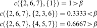
Here, the objects 2, 6, and 7 are included in the β-positive region as the set {2,6,7} is a β-subset of {2,3,6}. Calculating the subsets in this way leads to the following β-positive region:

Compare this with the positive region generated previously: {3,5}. Objects 2, 6, and 7 are now included due to the relaxation of the subset operator. Consider a decision table , where C is the set of conditional attributes and D the set of decision attributes. The β-positive region of an equivalence relation Q on U may be determined by:

A more comprehensive investigation of reducts for the VPRS approach may be found in Beynon (Reference Beynon2000, Reference Beynon2001), and Kryszkiewicz (Reference Kryszkiewicz1994). No general comparative studies appear to have been carried out with regard to comparing the rough set and the VPRS methods, although in Thangavel et al. (Reference Thangavel, Pethalakshmi and Jaganathan2006), the authors compare feature selection methods based on both RST and VPRS.

As indicated previously, the VPRS approach requires the specification of an additional parameter (β). This parameter can be approximated by repeated experimentation. However, problems may arise if searching for true reducts, as the VPRS approach incorporates an element of inaccuracy in determining the number of classifiable objects.

3.2 Tolerance rough sets

The TRSM (Skowron & Stepaniuk, Reference Skowron and Stepaniuk1996) can be useful for application to real-valued data. TRSM employs a similarity relation to minimize data as opposed to the indiscernibility relation used in classical rough sets. This allows a relaxation in the way equivalence classes are considered. The effect of employing this relaxation means that the granularity of the rough equivalence classes has been blurred slightly. This flexibility enables a change to occur in the boundaries of the former rough or crisp equivalence classes and objects may now belong to more than one so-called tolerance class which is TRSM equivalent of a rough set equivalence class.

The tolerance threshold (τ) is a global similarity threshold which determines the required level of similarity for inclusion within a tolerance class. The specification of this threshold, however, is a departure from the traditional rough set approach, which relies only upon the information contained in the data.

In this approach, suitable similarity relations must be defined for each feature, although the same definition can be used for all features if applicable. A standard measure for this purpose, given in Skowron and Stepaniuk (Reference Skowron and Stepaniuk1996), is:

(25)

where a is a considered feature, and a _max and a _min denote the maximum and minimum values of a, respectively. When considering the case where there is more than one feature, the defined similarities must be combined to provide an overall measure of similarity of objects. For a subset of features, P, this can be achieved in many ways, including the following approaches:

(26)

(27)

where τ is a global similarity threshold which determines the required level of similarity for inclusion within a tolerance class. The framework also allows for the specific case of traditional rough sets by defining a suitable similarity measure (e.g. complete equality of features) and threshold (τ = 1). Further similarity relations are summarized in Nguyen and Skowron (Reference Nguyen and Skowron1997a), but are not included here. From this, the tolerance classes that are generated by a given similarity relation for an object x are defined as:

(28)

Lower and upper approximations are defined in a similar way to those of traditional RST:

(29)

(30)

The tuple is known as a tolerance rough set (Skowron & Stepaniuk, Reference Skowron and Stepaniuk1994). Using this, the positive region and dependency functions can be defined as follows:

(31)

(32)

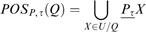
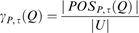
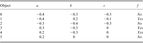
These definitions are analogous to the traditional rough set concepts and can be applied in the same way as demonstrated in Section 2.1.1. To demonstrate the approach, a sample data set is included in Table 2, which has three real-valued conditional attributes and a single crisp-valued decision attribute.

Figure 2

The FRNN algorithm (FRNN: U, the training data; C, the set of decision classes; y, the object to be classified)

Table 2

Real-valued data—example

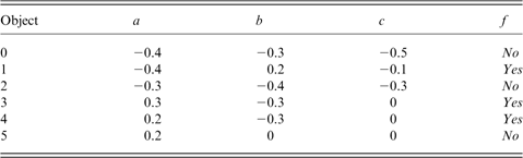
For this example, the similarity measure is the same as that given in 26 for all conditional attributes, with τ = 0.8. The choice of this threshold allows attribute values to differ to a limited degree, with close values considered as though they are identical.

Thus, by making A = {a}, B = {b}, C = {c}, and F = {f}, the following tolerance classes are generated:

It is apparent that some objects belong to more than one tolerance class. This is a result of employing a similarity measure rather than the strict equivalence of the conventional rough set model. Using these partitions, a degree of dependency can be calculated for attribute subsets, providing an evaluation of their significance in the same way as previously outlined for the crisp rough case.

From the lower approximation, the positive and boundary regions can then be generated thus:

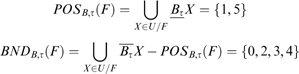
These concepts can be then employed in the same way as those of traditional rough sets to partition the data.

3.3 Dominance-based rough sets

The dominance-based rough set approach (DRSA; Greco et al., Reference Greco, Matarazzo and Slowiński2001) is an extension of RST for multi-criteria decision analysis. In contrast to traditional RST, DRSA employs a dominance relation instead of an equivalence relation. This allows DRSA to deal with the inconsistencies which are typical of criteria- and preference-ordered decision classes.

The ordering of data describing decision situations is naturally related to preferences of considered condition and decision attributes. Traditional RST does not have the ability to deal with ordinal data in the same way that DRSA does. This is because DRSA employs a dominance relation in place of the traditional rough set equivalence relation.

In DRSA, data are represented in decision table form. Let , where U is a non-empty set of finite objects, Q is a finite set of criteria, and , where V_q is the set of values that the criterion q can take, and is an information function such that for every . The set Q consists of condition criteria C, and the decision class D. Note that f(x,q) is the evaluation of object x on criterion , while f(x,d) is the decision class assignment for that object.

In order for DRSA to operate effectively on pre-ordered data, the approach employs a ‘preferencing’ or ‘outranking’ relation. A typical example is: _q; x _qy, which means that x is preferential to or ‘outranks’ y with respect to q. The values that q can take constitute a subset of real numbers—R, such that , and the preference relation is a simple order between real numbers ≥ such that x _qy f(x, q)≥f(y, q) holds. This relation is straightforward for a simple maximization criterion, for example, an exam result—‘the higher, the better’. For criteria where the opposite is true, for example, student failure-rate (‘the less, the better’), the relation can be satisfied by negated values of V_q. If , it can be said that x dominates y, denoted by xD_py, if x is ‘better’ than y for every criterion from P, x _qy, ∀q P. For each , the dominance relation D_P is reflexive and transitive. Given that ,

(33)

(34)

These are termed the P-dominating set and P-dominated set, respectively.

As the DRSA deals with ordinal data and objects, the manipulation of the data is carried out with respect to the ranking of decision classes. Let T = {1, … , n}. The domain values of decision criterion, V_{d ,} consist of n elements (it is assumed that V_d = T) and induce a partition of U into n classes Dc = {Dc_t, t∈T}, where . Each object is assigned to only one decision class Dc_t, t∈T. All of the classes are preference-ordered according to an increasing order of class indices, that is, ∀r, s∈T | r ≥ s, objects from are preferential to the objects from . Thus, the upward and downward unions of classes, respectively, can be defined as:

(35)

In DRSA, the knowledge being approximated is a collection of upward and downward unions of decision classes. The knowledge granules employed for approximation in DRSA are the P-dominating and P-dominated sets, which are analogous to the equivalence classes of traditional RST. The P-lower and the P-upper approximation of are denoted , respectively, and can be defined as follows:

(36)

(37)

Similarly, the P-lower and the P-upper approximation of , denoted by , respectively, can be defined thus:

(38)

(39)

As with traditional RST, the boundary regions of and can also be defined:

(40)

(41)

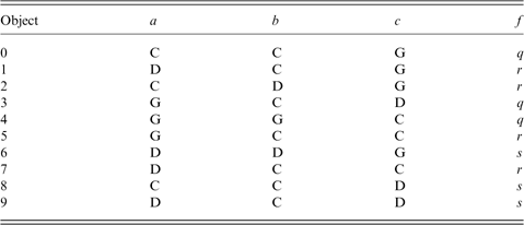
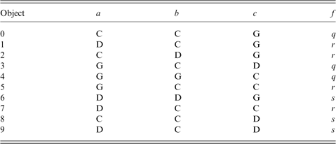
To demonstrate the basic concepts of the dominance rough set approach, a small example is shown here. The example data set in Table 3 has three conditional attributes (a, b, c) and one decision attribute (f) according to the decision attribute, the objects are divided into three preference-ordered classes: Cls1 = {q}, Cls2 = {r}, and Cls3 = {s}. Thus, the following unions of classes can be approximated:

Table 3

Dominance-based rough set approach—example

• • —the class of (at most) q objects

• • —the class of at most r objects

• • —the class of at least r objects

• • —the class of (at least) s objects

Figure 3

Example mammograms where breast tissue density increases from L-R corresponding to BIRADS class I (far left) to class IV (far right)

The lower approximations of the class unions consist of the following objects:

• • = {0, 4}

• • = {0, 1, 2, 3, 4, 5, 7} =

• • = {1, 2, 6, 7, 8, 9}

• • = {6, 8, 9} =

Therefore, only classes cannot be approximated without uncertainty. The upper approximations can be shown to be:

While the boundary regions for are:

These concepts can be used in a similar way to those of traditional RST in order to deal with ordinal data.

3.4 Vaguely quantified rough sets

In traditional RST, an object is a member of the upper approximation of a set if it is related to one of the elements in the set, while the lower approximation only retains those objects related to all the elements in the set. This is a result of the use of an existential quantifier in the definition of the upper approximation, and the use of a universal quantifier for the lower approximation. For real world data which include noise to a greater or lesser degree, this approach will inevitably suffer from classification errors and inconsistency. The associated definition of the upper approximation may be too general (thus resulting in very large sets), while the definition of lower approximation might be too rigid (resulting in an empty set in the extreme case). Fuzzy RST (which is covered in the next section) exhibits similar behaviour where the quantifiers ∃ and ∀ are replaced by the sup and inf operations (Cornelis et al., Reference Cornelis, De Cock and Radzikowska2007). These operators, however, can be as susceptible to the effects of noise as their crisp counterparts.

As demonstrated previously in Section 3.1, thresholds are introduced in VPRS to deal with these problems for the crisp case. In general, given 0 < l < u < 1, an element y is added to the lower approximation of a set A if at least (100 x u)% of the elements related to y are in A. Likewise, y belongs to the upper approximation of A if more than (100 x l)% of the elements related to y. This can be interpreted as a generalization of the rough set model using crisp quantifiers at least (100 x u)%, and more than (100 x l)% to replace the universal quantifier which demands rigid (at least 100%) membership for an element to be included in the lower approximation, and the existential quantifier which demands membership that is non-zero (greater than 0%) for an element to be included in the upper approximation.

In perhaps what is one of the most recent extensions of rough sets, the authors of (Cornelis et al., Reference Cornelis, De Cock and Radzikowska2007) introduce vague quantifiers like ‘most’ and ‘some’ to the rough set model. As a result of this, an element y now belongs to the lower approximation of A if most of the elements related to y are included in A. Similarly, an element belongs to the upper approximation of A if some of the elements related to y are included in A. In addition, the vague quantifiers are modelled mathematically in terms of the notion of fuzzy quantifiers in Zadeh (Reference Zadeh1965), so that the VQRS model inherits not only the flexibility of VPRS for dealing with classification errors mentioned previously, but also that of fuzzy sets for the expression of partial constraint satisfaction—by distinguishing between varying levels of membership of both the upper and lower approximations.

The definitions used for the upper and lower approximations in VPRS can be relaxed, through the use of vague quantifiers, to express that y belongs to the upper approximation of the set X to the extent that some elements of y’s equivalence class (Ry) are in the set A, and y belongs to the lower approximation of A to the extent that most elements of Ry are in X. In VQRS, it is implicitly assumed that the approximations are fuzzy sets, that is, mapped from X to [0, 1], that evaluate the degree to which the associated condition is fulfilled. The concept of a fuzzy quantifier in Zadeh (1965) is employed, that is, a [0, 1]→[0, 1] mapping Q. The set Q is said to be regularly increasing, if it is increasing and it satisfies the boundary conditions Q(0) = 0 and Q(1) = 1. Examples of fuzzy quantifiers can be generated by means of the following parameterized formula, for 0 ≤ α < β≤1, and x∈[0, 1],

(42)

For instance, Q _{(0.1, 0.6)} and Q _{(0.2, 1)} may be used to reflect the vague quantifiers some and most, respectively, from natural language.

The VQRS upper and lower approximations can be defined once the quantifier pair (Q _l, Q_u) has been fixed such that:

(43)

(44)

In other words, an element y belongs to the lower approximation of X if most of the elements related to y are included in X. Likewise, an element belongs to the upper approximation of X if some of the elements related to y are included in X. Notice that when X and R_P are a crisp set and a crisp equivalence relation, respectively, the approximations may still be non-crisp because of the use of vague quantifiers. In the interests of brevity, and due to significant overlap with fuzzy-rough sets, an example is not included here. Further detail and examples of VQRS, however, are covered in (Cornelis & Jensen, Reference Cornelis and Jensen2008).

3.5 Other rough set extensions

As mentioned previously, perhaps one of the most appealing aspects of traditional RST lies in its simplicity. It is based on straightforward set operations and is computationally efficient. Examining the concepts described earlier in Section 2.1, the most obvious areas for further exploration and extension are the equivalence relation and the subset operator, both of which are extended by the VPRS/VQRS and TRSM/DRSA approaches, respectively. One possible avenue for further exploration which has not been examined previously lies in a variable precision tolerance rough set approach. Although this would involve the specification of two parameters, it could take advantage of the benefits offered by both models: the ability to deal with real-valued data from TRSM and the ability to handle noise from the VPRS approach.

There is also one further aspect of RST, however, that is often overlooked: the upper approximation concept and its potential contribution to improving the performance of the rough set model. Work in this area has included an approach which generates reducts that preserve the rough upper approximation (Inuiguchi & Tsurumi, Reference Inuiguchi and Tsurumi2006), as well as an approach that considers the upper approximation and proposes a feature selection algorithm based on a rough upper approximation measure (Deogun et al., Reference Deogun, Raghavan and Sever1995).

Other techniques, such as those presented in Hu et al. (Reference Hu, Zhao, Xie and Yu2007a), Mac Parthaláin et al. (2007), and Mac Parthaláin and Shen (Reference Mac Parthaláin and Shen2009), consider the positive and boundary regions as conceptually different entities, and attempt to use the boundary region information for both feature selection and classification.

In particular, in Hu et al. (Reference Hu, Zhao, Xie and Yu2007a), the authors employ a consistency measure for feature selection in order to determine the classification of objects in the rough set boundary region and use this information to search for reducts. The approach uses a greedy-type search to select attributes which result in the greatest increase in the consistency value. Problems may arise, however, if the data on which the approach is operating are inconsistent; in these cases, a stopping threshold must be specified to avoid overfitting.

The approach in Mac Parthaláin et al. (2007), however, treats the data in the same way as those of traditional crisp RST. The central idea of this approach is that, from an intuitive point-of-view, objects in the boundary region of a given concept are more likely to belong to that concept if they are close to the objects of the positive region. Thus, a distance measure is employed to determine the ‘closeness’ or proximity of boundary region objects to those objects in the positive region. This proximity information is then used in feature selection as a measure to determine the ‘goodness’ or value of potential reducts.

An approach which examines the boundary region of tolerance rough sets (and thus can also handle real-valued data) based on Mac Parthaláin et al. (2007) has also been proposed (Mac Parthaláin & Shen, Reference Mac Parthaláin and Shen2009). Also, in Nguyen and Slezak (Reference Nguyen and Slezak2004), the authors discuss what they term ‘approximate reducts’, based on exploiting the rough set boundary. However, the work does not outline their application.

Another interesting idea which is explored in Slowinski and Vanderpooten (Reference Slowinski and Vanderpooten1997) and Slowinski and Vanderpooten (Reference Slowinski and Vanderpooten2000) is the re-definition of the upper and lower approximation concepts of RST. The definitions propose the use of fuzzy similarity, and tolerance, as opposed to indiscernibility, although otherwise the framework remains unchanged from that of traditional RST. Similar treatment is also given by the authors in Zhao and Zhang (Reference Zhao and Zhang2005) to VPRS to extend the β-upper and β-lower approximations; however, only similarity is explored in this case.

4.1 Rough set hybridizations

It has been demonstrated that RST can be very effective for preprocessing data input for neural networks (Jelonek et al., Reference Jelonek, Krawiec, Slowiński, Stefanowski and Szymas1994). More recent work (Mak & Munakata, Reference Mak and Munakata2002) has compared the rule extraction capabilities of both rough sets and neural networks and hybrid methods with ID3. The work of Yahia et al. (Reference Yahia, Mahmod, Sulaiman and Ahmad2000) further reinforces the utility of employing RST either as a neural network’s preprocessor or as a combined inference mechanism for medical diagnosis and is tested on a hepatitis disease data set. Another approach for medical image classification is reported in Shang and Shen (Reference Shang and Shen2002) that uses RST as a dimensionality reduction step before the application of a neural networks based classifier. Further detail with regard to the use of rough sets and hybrid methods for medical applications can be found in Pattaraintakorn and Cercone (Reference Pattaraintakorn and Cercone2007).

In Li and Wang (Reference Li and Wang2004), a hybrid rough set and neural networks approach for rule induction is presented. This technique is applied to relatively large data sets in order to generate more concise and accurate rules than either neural networks or rough sets alone. A feature selection algorithm is proposed and rules are generated from a decision table based on the rough set discernibility matrix. Reducts and rules are obtained using RST with neural networks employed to remove noisy data. Other rough set/neural network hybrid approaches are also to be found in Jelonek et al. (Reference Jelonek, Krawiec, Slowiński, Stefanowski and Szymas1994), Mitra and Banerjee (Reference Mitra and Banerjee1996), Swiniarski et al. (Reference Swiniarski, Hunt, Chalvet and Pearson1995), and Wang et al. (Reference Wang, Ding, Zhou and Zhang2005). In addition, it has been demonstrated that rough sets can help to generate new models of neurons in Lingras (Reference Lingras1996, Reference Lingras1997).

A review of the hybridization of RST with GAs is documented in Cordon et al. (Reference Cordon, Gomide, Herrera, Hoffmann and Magdalena2001). Prior to this, the first hybridization based on lower and upper bounds of numeric ranges was proposed as a rough-GA in Lingras and Davies (Reference Lingras and Davies2001). Others include: genetic encoding in order to generate rough set representations of clusters Lingras and West (Reference Lingras and West2004), and a hybrid decision support system for cancer detection Mitra and Mitra (Reference Mitra and Mitra2000). Genetic programming has also been allied with rough sets for bankruptcy classification McKee and Lensberg (Reference McKee and Lensberg2002).

RST has also been hybridized with classical statistical methods such as PCA (Swiniarski, Reference Swiniarski1999), Bayesian methods (Swiniarski, Reference Swiniarski1998), or wavelets (Wojdyllo, Reference Wojdyllo1998). Such integration has resulted in classifiers of better quality than those constructed through the use of RST alone (Browne et al., Reference Browne, Düntsch and Gediga1998).

In terms of hybridizing rough set extensions, a number of approaches have been proposed, such as fuzzy-rough VPRS (Mieszkowicz-Rolka & Rolka, Reference Mieszkowicz-Rolka and Rolka2004), and dominance-based rough sets and VPRS (Hu & Yu, Reference Hu and Yu2004). An interesting idea that has not yet been explored is a VPRS and TRSM hybrid. This would allow the flexibility to deal with real-valued data inherited from the TRSM approach and the noise tolerance of the VPRS method. This would mean the specification of two parameters, however, which would involve significant experimentation in order to establish ideal values for a given set of data.

4.2 Fuzzy-rough sets

FST was first proposed nearly 44 years ago (Zadeh, Reference Zadeh1965) and RST will celebrate its 28th anniversary this year (Pawlak, 1981). FST and RST complement one another (Dubois & Prade, Reference Dubois and Prade1992) and much advantage has been taken of this fact. This is reflected in the breadth and depth of research which has been undertaken in this particular hybridization of rough sets.

Note that fuzzy-rough sets should not be confused with existing approaches that directly combine the use of RST for dimensionality reduction and that of FST for knowledge modelling for example (Shen & Chouchoulas, Reference Shen and Chouchoulas2002; Shan et al., Reference Shan, Ishii, Hujun, Allinson, Freeman, Keane and Hubbard2002). Although successful in real-world applications, the underlying ideas of such work are straightforward and hence are omitted from the discussions below.

There have been two main lines of thought in the hybridization of fuzzy and rough sets: the constructive approach and the axiomatic approach. A general framework for the study of fuzzy-rough sets from both of these viewpoints is presented in (Yeung et al., Reference Yeung, Chen, Tsang, Lee and Xizhao2005). For the constructive approach, generalized lower and upper approximations are defined based on fuzzy relations. Initially, these were fuzzy similarity/equivalence relations (Dubois & Prade, Reference Dubois and Prade1992) but have since been extended to arbitrary fuzzy relations (Yeung et al., Reference Yeung, Chen, Tsang, Lee and Xizhao2005). The axiomatic approach is primarily for the study of the mathematical properties of fuzzy-rough sets (Wu & Zhang, Reference Wu and Zhang2004).

In (Dubois & Prade, Reference Dubois and Prade1992), the authors define the fuzzy P-lower and P-upper approximations as follows:

(45)

(46)

where F_i is a fuzzy equivalence class and X is the (fuzzy) concept to be approximated. The tuple is known as a fuzzy-rough set. Also in the literature are definitions for rough-fuzzy sets (Dubois & Prade, Reference Dubois and Prade1990; Srinivasan et al., Reference Srinivasan, Ruiz, Kraft and Chen1998), which can be seen as a particular case of fuzzy-rough sets. A rough-fuzzy set is a generalization of a rough set, derived from the approximation of a fuzzy set in a crisp approximation space. In (Yao, Reference Yao1997), it is argued that, in order to remain consistent, the approximation of a crisp set in a fuzzy approximation space should be called a fuzzy-rough set, and the approximation of a fuzzy set in a crisp approximation space should be called a rough-fuzzy set, thus ensuring that both models are complementary. In this framework, the approximation of a fuzzy set in a fuzzy approximation space is considered to be a more general model, unifying both theories. However, most researchers consider the traditional definition of fuzzy-rough sets in (Dubois & Prade, Reference Dubois and Prade1992) as standard. The specific use of min and max operators in the above definitions is expanded in (Radzikowska & Kerre, Reference Radzikowska and Kerre2002), where a wide range of fuzzy-rough sets are constructed, with each member represented by a particular implicator and t-norm. The properties of three typical implicators are investigated. Further investigations in this area can also be found in De Cock et al. (Reference De Cock, Cornelis and Kerre2004), Thiele, (Reference Thiele1998), Wu et al. (Reference Wu, Leung and Mi2005), Yeung et al. (Reference Yeung, Chen, Tsang, Lee and Xizhao2005).

In Boixader et al. (Reference Boixader, Jacas and Recasens2000), Morsi and Yakout, (Reference Morsi and Yakout1998), an axiomatic approach is taken, but is restricted to fuzzy T-similarity relations (and hence fuzzy T-rough sets). The properties of generalized fuzzy-rough sets are investigated in (Wu et al., Reference Wu, Mi and Zhang2003), and a pair of dual generalized fuzzy approximation operators are defined based on arbitrary fuzzy relations. The approach presented in (Mi & Zhang, Reference Mi and Zhang2004) introduces definitions for generalized fuzzy lower and upper approximation operators determined by a residual implication. Assumptions are found that allow a given fuzzy set-theoretic operator to represent a lower or upper approximation from a fuzzy relation. Different types of fuzzy relations produce different classes of fuzzy-rough set algebras.

The work in (Radzikowska & Kerre, Reference Radzikowska and Kerre2004) generalizes the fuzzy-rough set concept through the use of residuated lattices. An arbitrary residuated lattice is used as a basic algebraic structure, and several classes of lattice-valued fuzzy-rough sets (a fuzzy-rough hybridization of L-fuzzy sets) and their properties are investigated. In (Chen et al., Reference Chen, Zhang, Yeung and Tsang2006), a complete completely distributive (CCD) lattice is selected as the foundation for defining lower and upper approximations in an attempt to provide a unified framework for rough set generalizations. It is demonstrated that the existing fuzzy-rough sets are special cases of the approximations on a CCD lattice for T-similarity relations. The relationships between fuzzy-rough set models and fuzzy topologies on a finite universe have been investigated. The first such research was reported in (Boixader et al., Reference Boixader, Jacas and Recasens2000), where it was proved that the lower and upper approximation operators were fuzzy interior and closure operators, respectively, for fuzzy T-similarity relations. The work carried out in (Yeung et al., Reference Yeung, Chen, Tsang, Lee and Xizhao2005) investigated this for arbitrary fuzzy relations. In (Qina & Pei, Reference Qina and Pei2005) and (Wu, Reference Wu2005), it was shown that a pair of dual fuzzy rough approximation operators can induce a topological space if and only if the fuzzy relation is reflexive and transitive. The fuzzy interior (closure) operator is also examined.

In addition to the previous approaches to fuzzy-rough hybridization, other generalizations are possible. One of the first attempts at hybridizing the two theories is reported in (Wygralak, Reference Wygralak1989), where rough sets are expressed by a fuzzy membership function to represent the negative, boundary, and positive regions. All objects in the positive region have a membership of one and those belonging to the boundary region have a membership of 0.5, while those of the negative region have a membership of 0 as they do not belong to the set of interest. Thus, in adopting this approach, a rough set can be defined using FST. This also means that the rough set operators of union and intersection are modified accordingly. In (Pedrycz, Reference Pedrycz1999), the author attempts to address the problem where the fuzzy set representation of a rough set may be too precise, such that a concept is described exactly once its membership function has been defined. The solution to this is to employ an approximation of a family of fuzzy sets which the author terms a shadowed set. Shadowed sets do not use exact membership values but instead use truth values and a zone of uncertainty. A similar approach to that of (Wygralak, Reference Wygralak1989) is applied where elements may belong to a set with certainty (membership value 1), possibility (unit interval), or not belong (membership value 0). These ideas of course correspond to the rough set positive, boundary, and negative regions, respectively.

Another approach is reported in (Chimphlee et al., Reference Chimphlee, Abdullah, Sap, Srinoy and Chimphlee2006a) where the rough set lower approximation is employed, and elements are allowed to belong to this with certainty; however, the boundary region or uncertain region is fuzzified and membership values of elements are expressed in terms of a fuzzy membership function. The authors of (Mieszkowicz-Rolka & Rolka, Reference Mieszkowicz-Rolka and Rolka2004) apply a fuzzy-rough sets extension to the VPRS model described in Section 3.1 in an attempt to capitalize on the advantages of both rough sets and fuzzy sets within the VPRS framework. However, the VQRS approach of (Cornelis et al., Reference Cornelis, De Cock and Radzikowska2007) as detailed in Section 3.4 also takes advantage of these in a single approach as it employs fuzzy quantifiers and extends the VPRS approach simultaneously.

5.1 Classification

Classification concerns any problem in which a decision is taken or a forecast is made on the basis of available knowledge or information. A classification algorithm allows repeated forecasts to be made with regard to accumulated knowledge for new situations. Such algorithms can then be applied in order to classify previously unseen objects. Each new object can be assigned to a predefined set of classes, based on the observed values of suitably chosen attributes or features.

It is interesting to note that, despite the level of interest in rough set classification which is borne out by the number of publications in the area, no comprehensive survey of rough classification has been published to date. Perhaps this is due in part to the fact that RST is often married with other approaches when applied to the classification problem. Nevertheless, a number of RST-based classifiers have been proposed. The first application of RST to the classification problem is demonstrated in (Pawlak, Reference Pawlak1984). The authors (Pawlak & Skowron, Reference Pawlak and Skowron1993; Skowron, Reference Skowron1993; Slowinski et al., Reference Slowinski, Stefanowski and Siwinski2002) discuss the fundamentals of rough set rule induction for classification, but no algorithms are proposed.

The earliest RST-based classification algorithm is described in (Pawlak et al., Reference Pawlak, Slowinski and Slowinski1986). Later examples were proposed in (Bell & Guan, Reference Bell and Guan1998) and (Deogun et al., Reference Deogun, Raghavan and Sever1994), although the latter focused on database mining. Much use has been made of rough classifiers which were integrated into the learning from examples based on rough sets (LERS) framework (Grzymala-Busse & Grzymala-Busse, Reference Grzymala-Busse and Grzymala-Busse1995; Grzymala-Busse & Wang, Reference Grzymala-Busse and Wang1996). In these methods, descriptions of concepts are constructed through the calculation of all reducts for a given data set, by means of the decision rules. In (Bazan et al., Reference Bazan, Nguyen, Nguyen, Synak and Wroblewski2000), it is argued that these methods are not appropriate for classifying unseen data, and thus a number of rough set classification methods are proposed which address this problem. In addition, some new methods for rule induction from reducts, as well as ways of dealing with real-valued data discretization, are also described (also within the LERS framework). Similar aspects are also examined in Grzymala-Busse (Reference Grzymala-Busse2003) and Grzymala-Busse (Reference Grzymala-Busse2006). Other research such as (Stefanowski, Reference Stefanowski1998) also concentrates on addressing some of the shortcomings of the use of rough sets for rule induction as an aid to classification.

Rough set extensions have also been employed for classification. In (Ziarko, Reference Ziarko2003), the author discusses the use of VPRS for building decision tables from data models. Others which also employ VPRS include (Glymin & Ziarko, Reference Glymin and Ziarko2007) and (Zhao & Zhu, Reference Zhao and Zhu2006) for email spam filtering, and general classification (Zhao et al., Reference Zhao, Zhang and Pan2003). In (Wang et al., 2004), the authors have combined VPRS with fuzzy clustering techniques to discover rules in process planning. In the same way that VPRS has been applied to the classification task, so too has the TRSM, and a number of papers have been published in this area. Applications include handwriting classification (Kim & Bang, Reference Kim and Bang2000), web document classification (Yi et al., Reference Yi, Hu and Lu2005), and geographical land classification (Yun & Ma, Reference Yun and Ma2006). Although a relatively new approach, VQRS has also been applied to the classification of mammographic data (see Section 5 for further detail; Mac Parthaláin et al., Reference Mac Parthaláin, Jensen, Shen and Zwiggelaar2010). The DRSA has also been employed for rule induction (Shao & Zhang, Reference Shao and Zhang2004) and classification (Kotłowski et al., Reference Kotłowski, Dembczyński, Greco and Słowiński2008), albeit with application to ordinal data.

Initial attempts to use fuzzy-rough sets for classification were presented in (Sarkar, Reference Sarkar2000), which adopted a nearest neighbour (NN) type classifier approach. This approach attempted to handle both the fuzzy uncertainty due to overlapping classes and the rough uncertainty caused by a lack of informative features. A fuzzy-rough ownership function (a value which is influenced by all training objects) was employed in an effort to capture both of the aforementioned aspects. In addition, this also allows a possibilistic class membership assignment. The ownership function is influenced by all of the objects in the training set, which in turn means that the number of neighbours does not need to be defined. Other parameters must however be specified for successful operation. In (Wang et al., Reference Wang, Ding, Zhou and Zhang2005a), the authors extend the approach but divide the task of classification into four parts. First, using a leave-one-out type of strategy, the fuzzy-rough ownership value is calculated for each training object for all classes. The ownership value indicates the degree to which other objects support each individual object. Inconsistencies are then filtered from the training data—a high fuzzy-rough ownership value indicates a class other than a known class. Following this, representative points are selected from the processed training data and fuzzy-rough ownership values are refreshed based on mountain clustering. Then, finally, test objects are classified using only the representative training data from the previous step using the algorithm proposed in (Sarkar, Reference Sarkar2000).

Other NN classification methods which employ fuzzy-rough hybridization include (Bian & Mazlack, Reference Bian and Mazlack2003), which integrates rough uncertainty into the fuzzy kNN classifier using the definitions of fuzzy upper and lower approximations as defined in (Dubois & Prade, Reference Dubois and Prade1992). The membership of a test object to the upper and lower approximations for every class is determined by k NN. In addition, a similar approach is used in (Mac Parthaláin et al., Reference Mac Parthaláin, Jensen, Shen and Zwiggelaar2010); once again, the fuzzy-rough upper and lower approximations are used to determine the membership of test objects to a particular class.

Little research has taken place in the area of fuzzy-rough decision tree induction, although there is much interest in fuzzy decision trees because of their ability to model vagueness. The work on fuzzy-rough decision trees outlined in (Bhatt & Gopal, Reference Bhatt and Gopal2004) employs the fuzzy-rough ownership measure from (Sarkar, Reference Sarkar2000), which is used to define a ‘fuzzy-roughness’ measure and fuzzy-rough entropy measure. The node-splitting criterion is determined using the fuzzy-rough entropy measure. In (Jensen & Shen, Reference Jensen and Shen2008), a fuzzy decision tree algorithm based on the well-known fuzzy ID3 (Baldwin et al., Reference Baldwin, Lawry and Martin1997) approach is described. In this case, fuzzy-rough dependency is employed to decide when node splitting should occur. An approach for rule induction using fuzzy rough sets is proposed in (Hong et al., Reference Hong, Liou and Wang2006) for generating certain and possible rulesets from hierarchical data.

5.2 Clustering

The clustering task is the unsupervised classification of data objects (patterns observations, data vectors) into groups or clusters. Clustering has been addressed in many contexts and by researchers of many different disciplines, and this reflects its applicability and popularity as an important step in data analysis. Since both cluster analysis and RST form data groups, it is easy to see the conceptual similarity between the upper and lower approximation constructs of rough sets and formation of data clusters or groups. This similarity has meant that the rough sets lend themselves easily to the clustering problem. A further advantage that RST offers is that it may also provide scope for the discovery of ‘possible’ data clusterings through the use of the information contained in the rough set boundary region.

Much of the interest in rough clustering has been relatively recent (Hirano & Tsumoto, Reference Hirano and Tsumoto2000; Hirano & Tsumoto, Reference Hirano and Tsumoto2003; Peters et al., Reference Peters, Skowron, Suraj, Rzasa and Bokowski2002). The application of rough sets to clustering is not limited to the use of rough indiscernibility (Hirano & Tsumoto, Reference Hirano and Tsumoto2003). For instance, a rough set version of the classical k-means algorithm is proposed in (Lingras & West, Reference Lingras and West2004). Similarly, in (Lingras et al., Reference Lingras, Hogo and Snorek2004), Kohonen SOM (self-organizing maps) were used to generate intervals of clusters based on RST. The authors of (Malyszko & Stepaniuk, Reference Malyszko and Stepaniuk2008) propose a rough set clustering algorithm by combining entropy-based thresholding with rough sets.

The use of VPRS within the framework of the fuzzy c-means (FCM) algorithm (Bezdek, Reference Bezdek1981; Dunn, Reference Dunn1973) is documented in (Bao et al., Reference Bao, Han and Wu2006) where VPRS is employed to assign weights to each of the features. The basis for the approach is VPRS but an extension is proposed for the variable precision fuzzy-rough case. This is demonstrated by applying it to image analysis. VPRS is also used along with fuzzy-rough sets in (Zheng & Wang, Reference Zheng and Wang2008) as part of a fault diagnosis system. As an aid to fuzzy clustering in the general case in (Wang et al., Reference Wang, Shao, Zhang and Zhu2005b), VPRS is employed for generating rules from the fuzzy conditional and decision constructs of the fuzzy clustering algorithm. Although not as popular as traditional RST or VPRS, TRSM has been applied to the clustering problem in (Kawasaki et al., Reference Kawasaki, Nguyen and Ho2000) and (Ho & Nguyen, Reference Ho and Nguyen2002), where the authors employ an algorithm to cluster documents. Later work (Ngo & Nguyen, Reference Ngo and Nguyen2004) also used TRSM in a similar manner for clustering web search results. The traditional rough set approach is extended in (Kumar et al., Reference Kumar, Krishna, Bapi and De2007) by using a tolerance relation to form initial clusters; subsequent clusters are then formed using a constrained similarity relation which is also used as a merging criterion to combine initially identified clusters.

There have been few applications of fuzzy-RST to clustering. Most approaches, such as those of Wang et al. (Reference Wang, Shao, Zhang and Zhu2005b), mentioned previously, and Zhao et al. (Reference Zhao, Zhou and Tang2005), have tended to use both FST and RST but in isolation rather than in terms of fuzzy-RST. Rough-fuzzy sets are employed in Petrosino and Ceccarelli (Reference Petrosino and Ceccarelli2000) for texture separation in imaging, and in Pal (Reference Pal2004) the author also describes the application of rough-fuzzy sets for clustering and employs an image segmentation example to demonstrate this. In Chimphlee et al. (Reference Chimphlee, Abdullah, Sap, Srinoy and Chimphlee2006a), the authors propose a fuzzy-rough extension of the well-known FCM clustering algorithm and apply it to network security intrusion detection. Another fuzzy-rough approach which is also based on FCM is proposed in Hu and Yu (Reference Hu and Yu2005). It remains to be seen whether further fuzzy-rough approaches for clustering will be proposed, although it would seem that fuzzy-rough sets are well suited for such problems.

5.2.1 Document clustering

The clustering of documents is a difficult task for a number of reasons, mainly due to the textual characteristics and unstructured format that every individual document takes. In Ho et al. (Reference Ho, Kawasaki and Nguyen2006), the authors describe a method to cluster documents using tolerance rough sets. Two algorithms are described: one for hierarchical clustering and another for non-hierarchical clustering.

The approach can be broken down into two stages: the generation of tolerance classes, and the manipulation and generation of the clusters. In the first step shown below in Figure 4, a set of terms (words) is extracted from each document, and these are then assigned weights according to occurrence. Each individual term (t_i) is assigned a weight (w_i) which reflects its importance in the document; where i = 1, 2, 3,…,n with n being the number of extracted terms. A document is denoted by d_j = (t ₁, w _1j; t ₂, w _2j…; t_n, w_nj) and wiq∈[0, 1]. The weights are calculated by means of a frequency function, such that terms that occur often have a lower weight than those that rarely occur. This ensures that terms that occur in all documents have a zero weight. Each document is represented by a predefined number (R) of its highest weighted terms. All of the terms for all documents denoted by T are used in a co-occurrence matrix to determine how terms are related to one another. Using an uncertainty function derived from a tolerance relation, this matrix can then be used to generate tolerance classes of terms in T. It is at this point that the tolerance value (τ) must be specified for the uncertainty function.

Figure 4

Document clustering using tolerance rough sets—stage 1

In the second stage of the approach shown in Figure 5, a concept is defined which is used for the representation of clusters. This representation is what the authors term polythetic and must fulfil three properties which relate to the documents under consideration and the terms (words) in each document. Membership of each document to a cluster is defined in terms of a Bayesian minimum error rate and can be used to build each of the clusters. Cluster similarity is carried out in the usual manner, by employing a distance metric. It should be noted that clusters are built using only the upper approximation of the tolerance rough set calculated from a subset of terms X⊆T.

Figure 5

Document clustering using tolerance rough sets—stage 2

A number of experiments are conducted using both hierarchical and non-hierarchical clustering algorithms for both general clustering and information retrieval. In particular, the TRSM-based approach is compared with a vector space model (VSM) approach to clustering for information retrieval. This is an algebraic model for representing text documents as vectors of identifiers such as index terms. The TRSM-based method demonstrates that it can equal or outperform the VSM method. This, however, requires that a range of tolerance values are specified for the uncertainty function.

It is interesting to note that there are a number of areas of this approach that could be covered by using fuzzy-RST, thus eliminating the need for the subjective specification of the thresholding value of the TRSM. In addition, a number of other thresholds relating to the number of the terms, R, which should be considered for each document, could also be eliminated.

5.3 Feature selection

Feature selection (FS), which may also be referred to as attribute selection or semantics-preserving attribute reduction, is a term used to describe the problem of selecting input attributes that are most predictive of a given outcome. The FS problem is pervasive and can be encountered in many areas of machine learning, pattern recognition, and signal processing. In contrast to other methods for reduction of dimensionality, the FS approach preserves the original semantics or meaning of the features following reduction. FS has been applied to tasks that involve data sets which contain very large numbers of features (in the order of tens of thousands; Chouchoulas & Shen, Reference Chouchoulas and Shen2001). Without FS, such problems would prove to be computationally intractable.

As RST was originally proposed for supervised learning, it is no surprise, therefore, that one of the many successful applications of RST has been in the area of FS. The basic tenet of RST, which means that only the supplied data are employed for data reduction (with no additional information), has many benefits in FS. Most other methods require at least some supplementary knowledge. The main disadvantage of rough set-based FS in the literature is the restrictive requirement for all data to be crisp, and hence the motivation to extend the rough set model as described in Section 3.

There are two main approaches when searching for rough set reducts: the dependency degree approach and the discernibility matrix approach. Both approaches have been employed for rough set-based FS, although the discernibility matrix approach is computationally expensive for large data sets (Jensen & Shen, Reference Jensen and Shen2008), but some constructs (Pawlak, Reference Pawlak1991) have been proposed to alleviate this problem.

Among the earliest rough set-based dependency degree approaches to FS is the Preset algorithm (Modrzejewski, Reference Modrzejewski1993), which uses RST to rank features heuristically, within the assumption of a noise-free binary domain. In Zhong et al. (Reference Zhong, Dong and Ohsuga2001), a rough set heuristic filter-based approach is presented. The algorithm starts out by calculating the core of the data set (attributes that cannot be removed without introducing inconsistency) and then it incrementally adds attributes based on a heuristic measure. A threshold value is required as a stopping criterion to determine when a reduct candidate is sufficiently ‘close’ to being a reduct. In Chouchoulas and Shen (Reference Chouchoulas and Shen2001), the authors also present a filter-based method called rough set attribute reduction (RSAR), based on the rough set dependency degree. It uses a greedy forward selection technique (starting with an empty subset) that incrementally adds features that result in an increase in the dependency value. Other approaches have also utilized this approach but used other measures such as entropy (Jensen & Shen, Reference Jensen and Shen2004b) and a boundary region measure (Mac Parthaláin et al., 2007) to search for reducts. In terms of the discernibility matrix approach (Skowron & Rauszer, Reference Skowron and Rauszer1992), a number of techniques have also been proposed, and algorithms such as that described in Nguyen and Skowron (Reference Nguyen and Skowron1997a) adopt this technique to search for reducts. Others also include (Øhrn, Reference Øhrn1999) with specific application to medical problem domains, and (Wang & Wang, Reference Wang and Wang2001) which attempts to address the computational complexity associated with discernibility matrices.

Although not as popular as the traditional rough set approach, VPRS has also been applied to the FS problem. In Thangavel et al. (Reference Thangavel, Pethalakshmi and Jaganathan2006), the authors compare VPRS and traditional rough set-based FS techniques. A fault-detection process which uses VPRS as an FS step is also described in Li et al. (Reference Li, Wu, Zhang and Yue2006). The main disadvantage with approaches like VPRS is the specification of additional tunable parameters, in this case β. As mentioned previously, the optimum value can be obtained by repeated experimentation, but this may take considerable time depending on the nature of the data being examined.

Applying rough set-based FS to domains where the data are real-valued has previously meant that the data must be discretized beforehand. Tolerance rough sets have provided a solution to this problem, however, and in (Jensen & Shen, Reference Jensen and Shen2008) the authors demonstrate how this can be achieved. Unfortunately, the tolerance rough set approach requires a thresholding value which is specified by the user and can only be automatically approximated by repeated experimentation. Human specification of such a threshold, however, conflicts with the rough set ideology that only the information in the data should be employed. As mentioned previously, this has resulted in the development of techniques which extend the rough set concepts of the positive region and dependency function through the use of fuzzy sets resulting in a number of fuzzy-rough set approaches (Shen & Jensen, Reference Shen and Jensen2004; Jensen & Shen, Reference Jensen and Shen2004a, Reference Jensen and Shen2004b, Reference Jensen and Shen2007, Reference Jensen and Shen2008, Reference Jensen and Shen2009; Hu et al., Reference Hu, Xie and Yu2007b; Tsang et al., Reference Tsang, Chen, Yeung, Wang and Lee2008). A greedy hill-climbing search mechanism is then employed to search for subsets of features and a new fuzzy dependency measure is employed as a stopping criterion. In Hu et al. (Reference Hu, Yu and Xie2006), an approach that employs information measures for fuzzy indiscernibility relations is presented for the computation of feature importance. Reducts are then calculated by employing a greedy selection algorithm. Comprehensive coverage is given to fuzzy-rough FS approaches in Jensen and Shen (Reference Jensen and Shen2008), which explores all aspects of generation of reducts, and selection and search methods.

5.3.1 FS for gene expression data

The application of techniques such as machine learning, data mining, and pattern recognition to areas of Bioinformatics has enjoyed much attention in recent years, and rough sets and their extensions are no exception. One particular area within this field is the manipulation of gene expression data. Owing to the very large number of genes in the sample data, the search space is exponentially large, and thus any techniques which are applied to this type of data must be robust. Rough set techniques are therefore an ideal candidate for the examination of such data.

Rough set FS is employed in Momin et al. (Reference Momin, Mitra and Gupta2006) as a dimensionality reduction step and applied to a number of gene expression data sets. The FS step generates a number of reducts which are then used to reduce the data before they are classified using a NN approach. The approach can be described as a series of individual steps as shown in Figure 6. The first step involves discretizing the data such that it can be used with the rough set approach. This discretization step involves the search for partitions for each attribute domain. These partitions form new intervals to which objects can be assigned. A Bayesian equal-width approach is used in this case, which handles outliers in a sensible manner, but assumes uniform distribution of the data.

Figure 6

Feature Selection for gene expression data

Having discretized the data, the FS step is then implemented, using a heuristic search described below. The approach starts out with an empty set, to which those attributes that have a rough set dependency (γ > 0) are added incrementally. This generates a set of attributes from which reducts can later be generated. A thresholding value is also specified at this point termed λ; this value is used to limit the cardinality of all generated reducts. All possible reducts of cardinality λ are then generated, but only those of γ = 1 are retained. A pruning of all super sets of reducts is then carried out, and the data are reduced prior to the next step.

The next stage is data reduction where all of the reducts are used to minimize the data by selecting each of the features that appear in a given reduct from the data. Each reduced data set is then classified. The classifier used here is kNN (Keller et al., Reference Keller, Gray and Givens1985), which is an object-based classifier learner.

The above process is applied to four publicly available data sets relating to various types of cancer. Various values of λ are used to generate the reducts for each of the data sets which are then classified. For the kNN classifier, 3, 5, and 7 are selected for values of k, that is, the number of neighbours considered. Discovery of an optimal value for k, however, may take considerable time. A classification accuracy of 100% for all data sets is achieved for some but not all of the reducts generated. The process of generating such large numbers of reducts, however, is computationally expensive. The FS approach is compared with two other rough set approaches (Shen & Chouchoulas, Reference Shen and Chouchoulas2000) and (Zhong et al., Reference Zhong, Dong and Ohsuga2001), which also perform well; however, the authors argue that their method performs better on the basis of classification results.

Again, as with the application example in Section 5.2.1, what becomes apparent is the number of tunable parameters. Despite very high classification accuracies being achieved, these are subjective and can influence the final result. The authors mention a parameter for the discretization of the data, another for the FS approach, and of course k for the classification step. Note that if a hybrid fuzzy-rough approach rather than the current rough set approach were to be employed, the discretization step could be eliminated completely. This would also ensure that any potential loss of information would not occur due to the discretization step.