Introduction
The evolution toward 5G and future 6G communication systems has driven significant research into the millimeter-wave (mmWave) spectrum, which offers a broad bandwidth to support high-data-rate services [Reference Pant and Malviya1–Reference Andrews, Buzzi, Choi, Hanly, Lozano, Soong and Zhang3]. Phased array antennas, which possess beamforming capabilities, are an established and indispensable technology for overcoming the high path loss associated with mmWave frequencies [Reference Qu, Qu, Zhang, Yang and Chan4–Reference Chung, Lee, Hsu and Lin6].
However, the beam-scanning capability of phased arrays is still fundamentally hindered by the limited beamwidth of individual elements and the strong mutual coupling between them [Reference Yang, Li, Zhou and Qi7, Reference Yang, Zhang and Zhang8]. This coupling effect is exacerbated at wide scan angles, causing significant performance degradation [Reference Cheng, Ding, Shao and Wang9, Reference Elobied, Yang, Lou and Gao10]. To address these limitations, extensive research has focused on enhancing the scanning range of phased arrays through various strategies, including the use of wide-beam elements [Reference Yang, Cao, Gao, Yang and Li11, Reference Feng, Li, Zhang, Yu, Qi, Li and Zhou12], the integration of decoupling structures [Reference Wang, Tu, Yuan and Chen13, Reference Li and Xiao14], and the reduction of element spacing [Reference Fan and Wang15]. Nonetheless, achieving the demanding goal of ±50° wide-angle scanning in a compact and cost-effective configuration continues to be a key research challenge [Reference Jin, Sun, Liao, Wang, Cao, Che and Xue16].
The ridge substrate integrated waveguide (RSIW) has emerged as a highly suitable platform for wide-angle scanning phased arrays. Compared with substrate integrated waveguide (SIW), it combines the benefits of both ridge waveguides and SIWs, such as a lower cutoff frequency, a broader single-mode bandwidth, and a more compact size [Reference Moscato, Moro, Pasian, Bozzi and Perregrini17–Reference Ding and Wu19]. This compactness is particularly advantageous for array design, as it facilitates better control over element spacing and sidelobe levels. Moreover, the compact element size provides valuable physical space for integrating decoupling structures to suppress mutual coupling [Reference Wang, Zhong, Zhang and Liang20]. Furthermore, RSIW is more cost-effective than traditional waveguides and can be seamlessly integrated with planar circuits, such as printed circuit boards (PCBs).
Despite these advantages, realizing high-performance RSIW phased arrays with wide-angle scanning capability remains a challenging task that has not been fully addressed. A review of state-of-the-art methods indicates that many RSIW scanning arrays are based on the leaky-wave antenna (LWA) principle. Mallahzadeh and Mohammad-Ali-Nezhad [Reference Mallahzadeh and Mohammad-Ali-Nezhad21] presented a collinear slot antenna based on a double-ridged SIW. Although it achieves a peak gain of 11 dBi over a ±28° scan range, its beam direction is frequency dependent, which is a characteristic limitation of LWAs. An alternative approach is demonstrated in Wei et al. [Reference Wei, Li, Wang, Liu, Li and Wang22], which employs p-i-n diodes to reconfigure the radiating slots for fixed-frequency scanning. While this method expands the scanning range to ±52°, it comes at the cost of a significant 4.5 dB gain degradation at the scan edges. The limitations of both frequency-scanned and phase-tuned LWA topologies motivate the investigation of an RSIW phased array capable of delivering wide-angle scanning capabilities without compromising other critical performance metrics.
Different from previously published RSIW scanning arrays, a centerline collinear slot phased array is proposed in this paper. By periodically bending the RSIW ridge, a strong longitudinal current is induced along the RSIW centerline, thereby efficiently exciting the collinear slots for in-phase radiation. This centered arrangement preserves the overall structural symmetry, which is critical for suppressing cross-polarization. To address the challenge of mutual coupling, a via-based choke structure is also strategically integrated between the array elements to enhance isolation. On the basis of this method, a 1 × 4 linear array prototype operating in the n257 band was designed, fabricated, and measured. The experimental results demonstrate that the array achieves a wide impedance bandwidth of 10.7% (26.5–29.5 GHz), a high peak gain of 14.5 dBi, excellent inter-element isolation better than 19 dB, and a 3-dB beam scanning range exceeding ±50°. The proposed design presents an effective solution that combines wide-angle scanning capability with superior gain and isolation performance, making it a compelling candidate for 5G and future mmWave communication systems.
Design of a collinear slot phased array
Working principles of the RSIW with a bending ridge
The fundamental behavior of the RSIW, particularly its cutoff frequency, can be effectively understood using a resonance model. In this approach, the cross-section of the waveguide is modeled as a resonant circuit, as depicted in the transmission line model in Fig. 1.
RSIW equivalent circuit model.

The central ridge structure, formed by a row of metallic vias, introduces significant capacitive and inductive loading. An equivalent capacitance (C) is formed between the central vias of the ridge and the bottom ground plane. The vias themselves possess an intrinsic self-inductance, which is represented as an equivalent inductor (L). Together, these form a parallel L–C resonant circuit at the center of the waveguide. The sections of the waveguide on either side of the central ridge can be modeled as short-circuited transmission line stubs, each with a length of a/2, where a is the total width of the waveguide.
The core principle of this model is that the cutoff frequency (ωc) of the RSIW dominant mode corresponds to the resonant frequency of this entire transverse equivalent circuit. At resonance, the admittances of the central L–C tank and the two side stubs cancel each other out. This condition can be expressed by setting the total admittance at the central plane to zero:
 \begin{equation*}{Y_{LC}} + {Y_{stubs}} = 0\end{equation*}
where YLC is the admittance of the central L–C section, and Y stubs is the combined admittance of the two side stubs. This leads to the resonance equation:
 \begin{equation*}\frac{1}{{\frac{1}{{j\omega C}} + j\omega L}} - 2j{Y_0}{\text{cot}}\left( {{\beta _x}a/2} \right) = 0\end{equation*}
In this equation, βx is the propagation constant in the transverse direction. From this, βx can be derived as:
 \begin{equation*}{\beta _x} = \frac{2}{a}{\text{co}}{{\text{t}}^{ - 1}}\left[ {\frac{{\omega C}}{{2{Y_0}}}\left( {\frac{1}{{1 - {\omega ^2}LC}}} \right)} \right]\end{equation*}
The longitudinal propagation constant β for a wave traveling down the RSIW is then related to the transverse propagation constant βx by the standard waveguide equation:
 \begin{equation*}\beta = \sqrt {{\omega ^2}\mu \varepsilon - {{\left\{ {\frac{2}{a}{\text{co}}{{\text{t}}^{ - 1}}\left[ {\frac{{\mu ah{\omega ^2}C}}{{2\pi \left( {1 - {\omega ^2}LC} \right)}}} \right]} \right\}}^2}} \end{equation*}
Wave propagation is cut off when the longitudinal propagation constant β becomes zero. At this point, the electromagnetic wave no longer propagates along the transmission line but is confined to resonate in the cross-section. The cutoff frequency ωc is therefore found by setting β = 0 in the above equation, which yields the following transcendental equation:
 \begin{equation*}\begin{array}{*{20}{c}}
{{\omega _c}\sqrt {\mu \varepsilon } = \frac{2}{a}{\text{co}}{{\text{t}}^{ - 1}}\left( {\frac{1}{{2{Y_0}}}\frac{{{\omega _c}C}}{{1 - \omega _c^2LC}}} \right)} \\
{\theta = \frac{\pi }{2},\beta = 0,{\text{ }}{Y_0} = \frac{1}{h}\sqrt {\frac{\varepsilon }{\mu }} }
\end{array}\end{equation*}
This equivalent circuit model elucidates that the ridge structure acts as a capacitive load, effectively lowering the cutoff frequency compared to a standard waveguide of the same width. This allows for a more compact physical size for a given operating band, which is a key advantage of the RSIW topology.
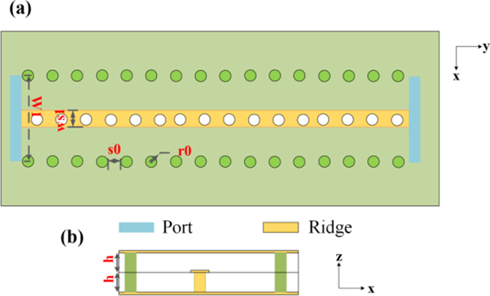
The proposed RSIW is realized via a standard PCB process. The stack-up consists of two layers of 0.813 mm-thick Rogers RT/duroid 4003 substrate (εr = 3.55, tanδ = 0.0027). The structure is bounded by top and bottom ground planes, which are equivalent to the top and bottom broad walls of the waveguides. Two rows of metallized via fences form the lateral walls, confining the electromagnetic field. A central ridge metal strip is patterned on the top surface of the lower substrate, and a single row of metallized vias connects the ridge metal strip and the bottom ground plane. In this configuration, the effective height of the ridge is determined by the substrate thickness (0.813 mm), which is a constraint imposed by the standard PCB fabrication process without blind vias.
The ridge configuration is primarily responsible for adjusting the cutoff frequency and impedance characteristics of the TE10 mode. The initial width parameters (W1, ws1) were estimated using the analytical cutoff frequency formula for a ridge waveguide. These two parameters were optimized via the HFSS with the dual objectives of maximizing the single-mode bandwidth to cover 26.5–29.5 GHz and minimizing the insertion loss. The height ratio between the ridge and the total waveguide was set to approximately 0.5, an empirical starting point known to provide favorable impedance characteristics. The final optimized dimensions are detailed in the caption of Fig. 2.
Schematic diagram of the RSIW configuration: (a) top view; (b) side view (dimensions: W1 = 3.4; ws1 = 0.7; s0 = 1; r0 = 0.5; h = 0.813 unit: mm).

Figure 2 Long description
RSIW configuration with two views is shown. In the top view, labeled as part (a), a rectangular layout is depicted with a central yellow ridge running horizontally. This ridge is flanked by two rows of green circles, representing elements, on either side. The ridge is marked with dimensions labeled W and ws1 in red. Two blue rectangles at the left and right edges represent ports. The labels s0 and r0 are positioned near the green circles, indicating specific points. An axis in the top right corner shows the x and y directions. In the side view, labeled as part (b), the ridge is shown in a cross-sectional view with the yellow ridge in the center. The height of the ridge is marked with h in red. The blue rectangles representing ports are visible at the ends. An axis in the bottom right corner indicates the x and z directions. The legend identifies the colors used for the port and ridge.
Figure 3(a) shows the cross-sectional electric field of the RSIW, which is tightly confined above the ridge and decays rapidly toward the sidewalls. In a conventional straight-ridge RSIW (Fig. 3(b)), the longitudinal surface current is null along the centerline because of symmetry. This prevents the direct excitation of any slot placed along the centerline. By periodically bending the ridge (Fig. 3(c)), the current is forced to follow the curved path, generating a nonzero longitudinal current that reaches its maximum at the apex of each curve. When collinear slots are etched with their centers precisely aligned at the current maxima, each slot radiator is efficiently excited.
(a) Schematic diagram of the cross-sectional electric field of the RSIW. (b) Surface current distribution with a straight ridge. (c) Surface current distribution with a bent ridge.

Figure 3 Long description
Cross-sectional electric field of the RSIW, with arrows indicating the direction of the field. The field is tightly confined above the ridge and decreases rapidly toward the sidewalls. Surface current distribution with a straight ridge. The diagram includes a color scale on the left labeled J subscript surf left bracket A divided by m right bracket, ranging from 0 to 300. The surface current is null along the centerline due to symmetry, preventing direct excitation of slots placed along the centerline. Surface current distribution with a bent ridge. The same color scale is present on the left. The current follows a curved path, generating a nonzero longitudinal current that reaches its maximum at the apex of each curve. Collinear slots are etched with their centers aligned at the current maxima, efficiently exciting each slot radiator.
Design of the GCPW-RSIW transition
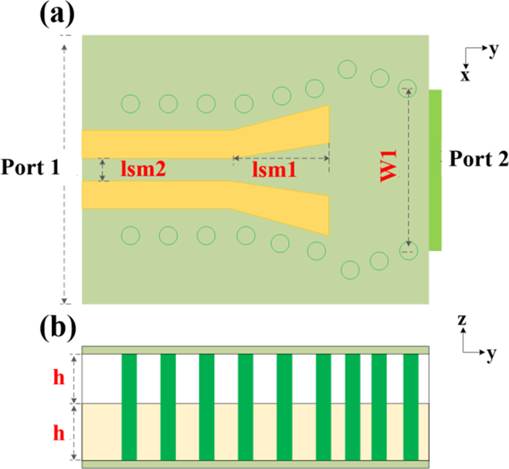
To provide a standard 50 Ω interface for measurement and system integration, a planar GCPW-RSIW transition was codesigned on the same Rogers RT/duroid 4003 substrate. As illustrated in Fig. 4, power is coupled from the GCPW port and efficiently guided into the main RSIW section that feeds the radiating slots. After optimization for both wideband matching and low insertion loss, the final dimensions were determined (see caption of Fig. 4).
Schematic diagram of the grounded coplanar waveguide (GCPW)-RSIW transition: (a) top view; (b) side view (dimensions: lsm1 = 2.5; lsm2 = 0.63 unit: mm).

Figure 4 Long description
The schematic consists of two parts labeled (a) and (b). In part (a), the top view shows a grounded coplanar waveguide (GCPW) to rectangular substrate integrated waveguide (RSIW) transition. Port 1 is on the left, and Port 2 is on the right. The transition features a tapered section with dimensions labeled as lsm1 and lsm2, and a width labeled W1. Circular elements are arranged around the tapered section. Part b presents the side view, showing alternating layers with height labeled h. The coordinate axes x, y, and z are indicated in both views, with x and y in the top view and y and z in the side view.
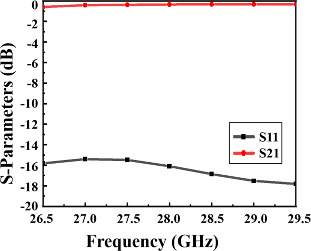
The simulated S-parameters validate the effectiveness of the design. As shown in Fig. 5, across the entire operational band, the input reflection coefficient S11 remains consistently below −15 dB, whereas the insertion loss S21 is better than 0.6 dB.
Simulated S-parameters of the GCPW-RSIW transition.

Design of the antenna subarray
The slot antenna is designed as a standing-wave, series-fed slot array. To achieve this, the waveguide is terminated with a short circuit. The first slot is positioned approximately a quarter of a guided wavelength (λg₀/4) from the short-circuited end to align with a current maximum of the standing wave. Subsequent slots are spaced by approximately half a guided wavelength (λg₀/2). This spacing ensures that each slot is located at a successive current maximum, leading to in-phase radiation from all elements and forming a broadside beam. The guided wavelength (λg₀) at the center frequency was calculated using the standard formula:
 \begin{equation*}{\lambda _{g0}} = \lambda \sqrt {1 - {{\left( {\frac{\lambda }{{{\lambda _c}}}} \right)}^2}} \end{equation*}
where λ 0 is the free-space wavelength, and λc is the cutoff wavelength of the designed RSIW.
As shown in Fig. 6, the subarray, which serves as the fundamental element of a larger phased array, consists of four collinear slots etched along the centerline of the ridge-bent RSIW. Each slot center is precisely aligned with the apex of the curvature, where the longitudinal surface current is maximal, ensuring efficient excitation. The transverse currents are symmetric with respect to the slot, leading to cancellation of their far-field contributions and thus low cross-polarization levels.
Schematic diagram of the collinear slot subarray: (a) exploded view; (b) top view (dimensions: Ls = 3.24; Ws = 0.63; ds = 3.95; sp = 2.12; sp_port = 1.42; ds_RW = 1 unit: mm).

Figure 6 Long description
The image consists of two parts. The first part, labeled (a), is an exploded view of a collinear slot subarray. It shows multiple layers with slots on the top layer, ports on the middle layer, and metallized vias connecting the layers. The bottom layer is labeled as metal. An axis is shown with x, y, and z directions. The second part, labeled (b), is a top view of the subarray. It displays a central ridge with slots labeled as Ls, ds, and sp, and ports labeled as sp_port. Metallized vias are represented as circles along the edges. The x and y axes are indicated, showing the orientation of the subarray.
The choice of four radiating slots offers a good compromise between achieving sufficient element gain and maintaining a wide half-power beamwidth (HPBW), which is necessary to permit a large scan range for the assembled phased array with minimal scan loss. The subarray performance was fine-tuned through the optimization of several geometrical parameters. The slot length Ls primarily dictates its resonant frequency, whereas the slot width Ws and slot offset ds_RW govern the radiation strength and impedance of each slot, thereby impacting the overall impedance matching of the subarray. The final geometrical parameters are listed in the caption of Fig. 6.
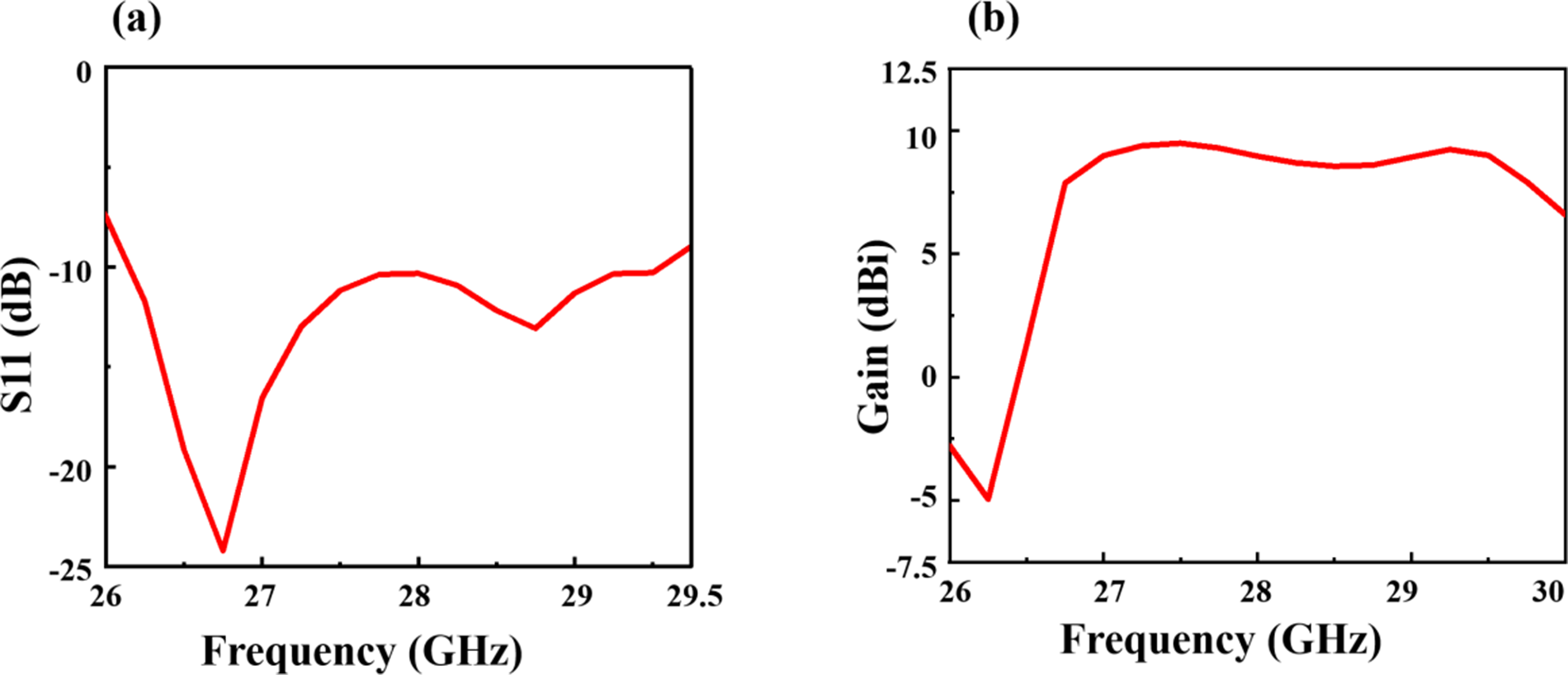
As depicted in Fig. 7(a), the subarray achieves an impedance bandwidth of 26.5–29.5 GHz, corresponding to a relative bandwidth of 10.6%. The realized gain within this band is shown in Fig. 7(b), which exceeds 7.5 dBi across most frequencies. The slight gain reduction at lower frequencies is a residual effect of the series-fed topology, where minor beam squint causes the peak gain to shift slightly. Figure 8 presents the performance of the subarray at 26.75, 28, and 29.5 GHz. Examination of the XOZ plane (E-plane) radiation patterns reveals that the HPBW of the subarray is consistently above 95°. The radiation patterns exhibit excellent symmetry, and the cross-polarization level is below −20 dB in the E-plane.
Simulated performance of the collinear slot subarray: (a) S11; (b) gain.

Simulated radiation pattern of the collinear slot subarray: (a) 26.75 GHz, (b) 28 GHz, and (c) 29.5 GHz.

Figure 8 Long description
Three polar plots labeled a, b, and c show angular radiation patterns with two overlaid traces identified in the legend as X-Pol and Co-pol. Common axes and ticks for a, b, and c: The angular scale is marked at 0, 30, 60, 90, 120, 150, 180, 210, 240, 270, 300, and 330. The radial quantity label is vertical bar E vertical bar decibel. Radial tick labels shown are 20, 0, minus 20, minus 40, and minus 60. Sub-image a: The Co-pol trace forms an outer loop that is closest to the 20 ring near 0 and remains near the outer rings through most angles, with a visible inward dip centered near 180. The X-Pol trace is a dashed inner loop with multiple lobes; it stays inside the Co-pol trace and lies mostly between the minus 20 and minus 40 rings, with deeper inward sections approaching the minus 60 ring. Sub-image b: The Co-pol trace forms an outer loop similar in overall size to sub-image a, with an inward dip near 180. The X-Pol trace is a dashed inner loop that is more circular than in sub-image a and remains inside the Co-pol trace, lying mostly between the minus 20 and minus 40 rings. Sub-image c: The Co-pol trace forms an outer loop with an inward dip near 180. The X-Pol trace is a dashed inner loop that is closer to circular than in sub-image a and shows a visible indentation near 180, remaining inside the Co-pol trace and lying mostly between the minus 20 and minus 40 rings.
Assembly of the phased array
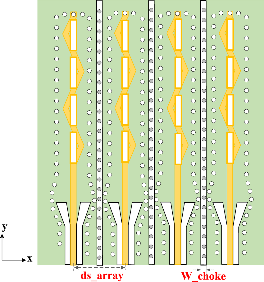
The assembled 1 × 4 phased array is depicted in Fig. 9. The element spacing ds_array is a trade-off between two competing factors: the avoidance of grating lobes and the minimization of mutual coupling. Theoretical analysis dictates the upper limit for the spacing. To achieve a grating-lobe-free scan range of ±60°, the element spacing ds_array must satisfy the condition ds_array <λ₀/(1 + sin(60°)), which is approximately 0.535λ₀, where λ₀ is the free-space wavelength at the center frequency. Conversely, the lower limit is constrained by mutual coupling. An excessively small spacing leads to strong mutual coupling between elements, which can degrade impedance matching and distort the radiation patterns. To balance this trade-off, an element spacing ds_array of 5.3 mm was selected, which corresponds to approximately 0.5λ₀ at 28 GHz.
Schematic diagram of the 1 × 4 phased array.

Figure 9 Long description
A schematic diagram of a 1}4 phased array features four vertical elements arranged in parallel. Each element consists of radiating sections and feed structures, represented by rectangular and diamond-shaped patterns. The spacing between elements is labeled 'dsarray', indicating the distance that controls grating lobes and mutual coupling. Vertical lines labeled 'Wchoke' represent choke structures that manage impedance and radiation patterns. An x superscript subscript –y axis indicator shows x as horizontal and y as vertical. The background grid of small circles may suggest a substrate or structural pattern, though its technical relevance is not specified. The diagram illustrates the spatial arrangement and functional components of the phased array, emphasizing the importance of element spacing and choke width in antenna performance.
To further mitigate the mutual coupling at this 0.5λ₀ spacing and thus improve the scanning performance, a decoupling structure was integrated between the subarrays. Owing to the planar fabrication process, a conventional three-dimensional (3D) choke is impractical. Therefore, an equivalent choke structure was realized by implementing a row of periodically arranged metallized vias into the ground plane between adjacent subarrays. This structure acts as a surface wave bandgap, suppressing unwanted propagation between subarrays. The width of this choke W_choke is set to 0.5 mm, and the overall dimensions of the array antenna are 2.15 × 2.5 × 0.17λ₀ @28 GHz.
To achieve electronically controlled 1D scanning, the array is excited by four feed ports with equal amplitudes. A progressive phase shift is applied between adjacent subarrays, which steers the main beam. As illustrated in Fig. 10(a), the reflection coefficient S11 remains below −10 dB across the 26.5–29.5 GHz band, corresponding to a 10.7% bandwidth and covering the 5G n257 band. The simulations of the transmission coefficients, shown in Fig. 10(b), reveal that the isolation between adjacent ports (1–2, 2–3, 3–1, and 4–1) is better than −16 dB across the band. The envelope correlation coefficient (ECC) was evaluated using embedded element far-field patterns, as shown in Fig. 10(c). Within 26.5–28.5 GHz, all ECC values remain below 0.01, indicating excellent port isolation and radiation pattern diversity. A noticeable increase in ECC is observed above 29 GHz, suggesting degradation near the upper band edge.
Simulated performance of the 1 × 4 phased array: (a) reflection coefficient, (b) port isolation, and (c) envelope correlation coefficient.

Figure 10 Long description
Line plot A with the y-axis labeled S-Parameters (decibel) and the x-axis labeled Frequency (gigahertz). The x-axis runs from 26.5 to 30.0 with labeled ticks at 26.5, 27.0, 27.5, 28.0, 28.5, 29.0, 29.5, and 30.0. The y-axis shows labeled ticks at minus 6, minus 8, minus 10, minus 12, and minus 14. A legend lists S11, S22, S33, and S44. All four traces start near about minus 10 at 26.5, drop to around minus 14 near 26.7, rise to around minus 12 near 27.0 to 27.5, rise to around minus 10 to minus 11 near about 28.0 to 28.3, then fall to around minus 12 near about 28.6 to 29.0, and continue around minus 12 to minus 14 through about 29.5, ending near about minus 12 to minus 13 at 30.0. Line plot B with the y-axis labeled Isolation (decibel) and the x-axis labeled Frequency (gigahertz). The x-axis runs from 26.5 to 30.0 with labeled ticks at 26.5, 27.0, 27.5, 28.0, 28.5, 29.0, 29.5, and 30.0. The y-axis shows labeled ticks at minus 15, minus 20, minus 25, minus 30, and minus 35. A legend lists S21, S32, S41, and S31. S21 and S32 are near minus 21 to minus 22 at 26.5, rise to around minus 16 to minus 17 by about 27.0 to 28.5, then drop to around minus 20 to minus 22 near about 29.0 to 29.5, and end near about minus 21 at 30.0. S31 stays around minus 25 to minus 21 from 26.5 to about 28.5, drops to around minus 24 near about 29.0, and stays near about minus 24 to minus 23 through 30.0. S41 drops to about minus 35 near about 26.7, rises to around minus 29 near about 27.5, rises to around minus 25 to minus 26 near about 28.3 to 28.6, then falls to around minus 28 to minus 29 near about 29.0 to 30.0. Line plot C with the y-axis labeled Envelope Correlation Coefficient and the x-axis labeled Frequency (gigahertz). The x-axis runs from 26.5 to 29.5 with labeled ticks at 26.5, 27.0, 27.5, 28.0, 28.5, 29.0, and 29.5. The y-axis ranges from minus 0.02 up to 0.16 with labeled ticks at minus 0.02, 0.00, 0.02, 0.04, 0.06, 0.08, 0.10, 0.12, 0.14, and 0.16. A legend lists ECC12, ECC13, ECC14, ECC23, ECC24, and ECC34. All traces stay close to 0.00 from 26.5 to about 28.4, with a small dip below 0.00 near about 28.3 to 28.5. From about 28.6 to 29.0, several traces rise to peaks around 0.02 to 0.09 near about 29.0. From about 29.0 to 29.5, multiple traces increase further, with the highest trace reaching about 0.15 at 29.5, while another ends near about 0.12 at 29.5, and at least one trace drops back toward about 0.00 by 29.5.
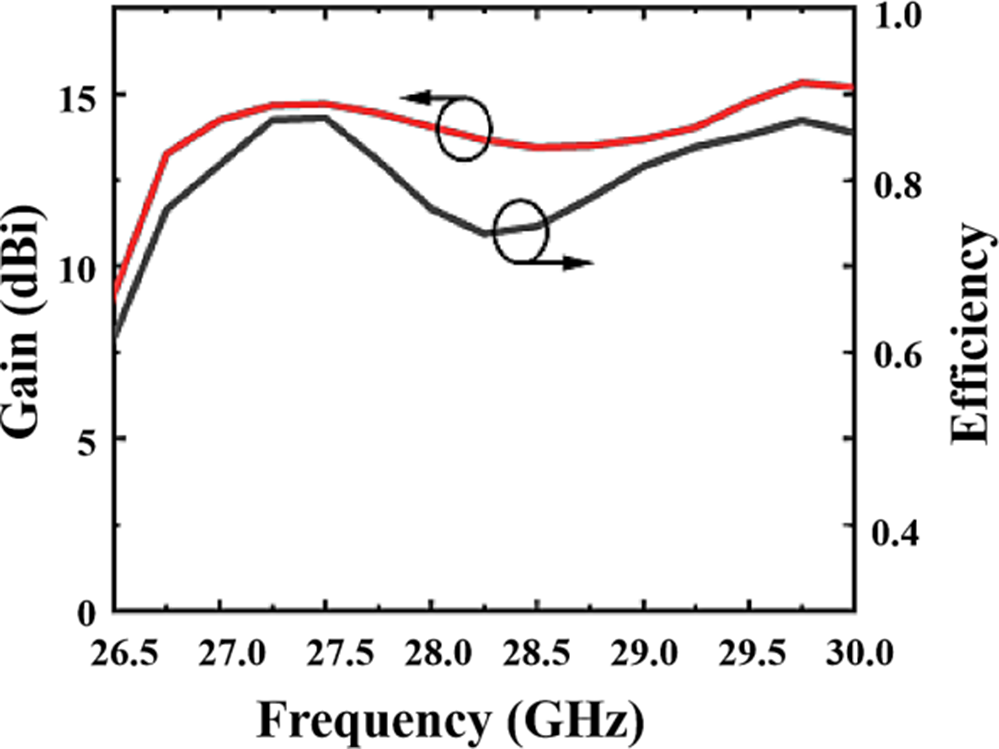
As depicted in Fig. 11, the array’s broadside realized gain is 13.2 dBi at 26.75 GHz and increases to 14.77 dBi at 29.5 GHz. The radiation efficiency, accounting for metal and dielectric losses, exceeds 70% across most of the operating band.
Simulated gain and efficiency of the 1 × 4 phased array.

The scanning performances of the 1 × 4 array at 26.75, 28, and 29.5 GHz are presented in Fig. 12. The gain decreases smoothly as the beam is steered away from the broadside. Specifically, at 28 GHz, 3-dB gain roll-off occurs at a scan angle of ±50°. At the band edges (26.75 and 29.5 GHz), the scan ranges for a 3-dB gain roll-off are ±52° and ±50°, respectively, demonstrating wide-angle scanning capability across the entire operational bandwidth.
Simulated directivity of a 1 × 4 phased array: (a) E-plane scan at 26.75 GHz; (b) E-plane scan at 28 GHz; and (c) E-plane scan at 29.5 GHz.

Figure 12 Long description
Directivity (dBi) versus Theta (deg) with multiple overlaid line series. The x-axis is labeled Theta (deg) and runs from minus 200 to 200 with labeled ticks at minus 200, minus 100, 0, 100, 200. The y-axis is labeled Directivity (dBi) and runs from minus 25 to 15 with labeled ticks at minus 25, minus 20, minus 15, minus 10, minus 5, 0, 5, 10, 15. Two vertical lines mark Theta equals minus 52 degrees and Theta equals 52 degrees, with the labels minus 52 degree and 52 degree near the top. Legend entries list: 26.75GHz minus 20 degree Scan; 26.75GHz 0 degree Scan; 26.75GHz 20 degree Scan; 26.75GHz 40 degree Scan; 26.75GHz 52 degree Scan; 26.75GHz minus 52 degree Scan; 26.75GHz minus 40 degree Scan. The plotted curves show a main lobe region between the two vertical lines with peaks near the top of the axis (around 10 to 15 dBi) and multiple narrow dips and oscillations near the center around Theta near 0 degrees. Outside the marked region, the curves drop and oscillate, reaching values below 0 dBi and down toward about minus 20 dBi in several places. Directivity (dBi) versus Theta (deg) with multiple overlaid line series. The x-axis is labeled Theta (deg) and runs from minus 200 to 200 with labeled ticks at minus 200, minus 100, 0, 100, 200. The y-axis is labeled Directivity (dBi) and runs from minus 35 to 15 with labeled ticks at minus 35, minus 30, minus 25, minus 20, minus 15, minus 10, minus 5, 0, 5, 10, 15. Two vertical lines mark Theta equals minus 50 degrees and Theta equals 50 degrees, with the labels minus 50 degree and 50 degree near the top. Legend entries list: 28GHz 0 degree Scan; 28GHz 20 degree Scan; 28GHz 40 degree Scan; 28GHz 50 degree Scan; 28GHz minus 50 degree Scan; 28GHz minus 40 degree Scan; 28GHz minus 20 degree Scan. The curves form a broad main lobe between the vertical lines with peaks near the top of the axis (around 10 to 15 dBi) and many narrow notches near the center around Theta near 0 degrees. Several curves outside the marked region fall below minus 10 dBi, with some deeper troughs approaching the lower part of the axis. Directivity (dBi) versus Theta (deg) with multiple overlaid line series. The x-axis is labeled Theta (deg) and runs from minus 200 to 200 with labeled ticks at minus 200, minus 100, 0, 100, 200. The y-axis is labeled Directivity (dBi) and runs from minus 30 to 20 with labeled ticks at minus 30, minus 25, minus 20, minus 15, minus 10, minus 5, 0, 5, 10, 15, 20. Two vertical lines mark Theta equals minus 50 degrees and Theta equals 50 degrees, with the labels minus 50 degree and 50 degree near the top. Legend entries list: 29.5GHz 0 degree Scan; 29.5GHz minus 20 degree Scan; 29.5GHz minus 40 degree Scan; 29.5GHz minus 50 degree Scan; 29.5GHz 50 degree Scan; 29.5GHz 40 degree Scan; 29.5GHz 20 degree Scan. The curves show a main lobe between the vertical lines with peaks near about 10 to 15 dBi and multiple narrow dips near the center around Theta near 0 degrees. Outside the marked region, the curves oscillate and drop below 0 dBi, with several troughs reaching toward about minus 25 dBi.
Measurement and performance comparison
To validate the performance of the proposed collinear slot phased array, a prototype was fabricated using a Rogers RT/duroid 4003 dielectric substrate with a single-layer thickness of 0.813 mm. The array features a simple structure, with all the elements integrated on two dielectric substrates, which were bonded together via the RO4450F adhesive. The fabrication process relies solely on PCB technology, offering significant cost advantages. A photo of the fabricated prototype is shown in Fig. 13.
Fabricated prototypes of the (a) subarray and (b) 1 × 4 phased array.

The ports of the 1 × 4 array were securely mounted to 2.92 mm connectors with a characteristic impedance of 50 Ω. The matching and radiation characteristics of the antenna were assessed via a vector network analyzer (R&S ZVA67 VNA) and an MVG Satimo StarLab microwave chamber. Given that the element spacing for the BBOX BB-ONE-JF-28- digital phase shifter (4 × 4/8 × 8) is ∼5 mm, the antenna was directly connected to the phase shifter during testing, as shown in Fig. 14. Notably, owing to a mounting flange on the chamber turntable that obstructed the rear hemisphere, only the forward radiation performance (from −90° to +90°) could be reliably measured.
Measurement setup for (a) S-parameter and (b) gain.

The measured S-parameters and radiation characteristics of the fabricated subarray prototype were compared against the simulation results. Figure 15 presents a comparison of the measured and simulated reflection coefficients S11. The measured S11 shows good agreement with the simulation across the majority of the target frequency band. A deviation is observed at the lower band edge, where the measured S11 is slightly above −10 dB. This discrepancy is attributed primarily to the impedance mismatch introduced by the solder transition between the 2.92 mm connector and the feed port of the antenna, which is a common factor for prototypes at these frequencies. Minor fabrication tolerances may also be a contributing factor.
Simulated and measured S11 of the subarray.

The measured and simulated realized gains are compared in Fig. 16. The measurement results confirm a stable gain profile across the frequency band. The measured gain tracks the simulated curve closely, with a maximum deviation of less than 1 dB observed at the lower band edge. This level of agreement is well within acceptable margins and validates the subarray performance.
Simulated and measured gains of the subarray.

Figure 17 shows a comparison of the normalized radiation patterns in the XOZ-plane (E-plane) at 26.75, 28, and 29.5 GHz. Excellent agreement is observed between the measured and simulated patterns. Key features such as the main lobe shape and the HPBW are accurately reproduced in the measurement. The minor discrepancies in side-lobe levels can be attributed to the test environment and manufacturing tolerances.
Normalized radiation patterns of the subarray at (a) 26.75 GHz, (b) 28 GHz, and (c) 29.5 GHz.

Figure 17 Long description
A showing a polar plot of vertical bar E vertical bar in decibel versus angle in degrees. Angle labels are 0, 30, 60, 90, 120, 150, 180, 210, 240, 270, 300, 330. The radial scale is labeled 10, 0, minus 10, minus 20, minus 30, minus 40, minus 50, minus 60, with higher values farther from the center. The legend lists Sim. X-pol, Sim. Co-pol, Meas. X-pol, Meas. Co-pol. Sim. Co-pol stays near the 10 ring from about 0 through 150 degrees and from about 210 through 360 degrees, and dips inward near 180 degrees to around the 0 ring. Meas. X-pol follows inside Sim. Co-pol, near the 0 ring around 0 degrees, and drops inward near 180 degrees to around the minus 20 ring. Meas. Co-pol is a broken curve mostly between the minus 10 and minus 30 rings around many angles, with segments dipping toward about the minus 40 ring near 180 degrees. Sim. X-pol is a broken curve closer to the center, mostly between the minus 30 and minus 50 rings. B showing a polar plot of vertical bar E vertical bar in decibel versus angle in degrees, with the same angle labels 0 to 330 in steps of 30 and the same radial labels 10 to minus 60. The legend lists Sim. X-pol, Sim. Co-pol, Meas. X-pol, Meas. Co-pol. Sim. Co-pol is near the 10 ring around most angles and dips near 180 degrees to around the 0 ring. Meas. X-pol is close to the outer loop near the 10 ring around 0 degrees and shows a deeper inward notch near 180 degrees reaching about the minus 20 ring. Sim. X-pol forms an inner broken loop around the minus 30 ring. Meas. Co-pol forms a broken loop mostly between the minus 20 and minus 40 rings, with a deeper inward feature near 180 degrees approaching about the minus 50 ring. C showing a polar plot of vertical bar E vertical bar in decibel versus angle in degrees, with the same angle labels 0 to 330 in steps of 30 and the same radial labels 10 to minus 60. The legend lists Sim. X-pol, Sim. Co-pol, Meas. X-pol, Meas. Co-pol. Sim. Co-pol is near the 10 ring around most angles and dips near 180 degrees to around the 0 ring. Meas. Co-pol runs just inside Sim. Co-pol, near the 0 ring around 0 degrees, and dips near 180 degrees to around the minus 10 to minus 20 region. Meas. X-pol is a broken curve mostly between the minus 10 and minus 40 rings, with multiple inward spikes and a deeper inward region near 180 degrees reaching about the minus 50 ring. Sim. X-pol is a broken curve closer to the center, forming an inner loop mostly between the minus 30 and minus 50 rings.
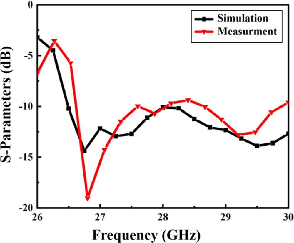
The fabricated 1 × 4 phased array prototype was measured and compared against the simulation results to validate its performance. The four ports are driven simultaneously with equal amplitudes and controlled phase shifts to synthesize a single beam for electronic steering instead of transmitting independent data streams from uncorrelated ports. Figure 18 compares the measured and simulated reflection coefficients S11 for the center port of the array. The measured results show a similar resonant performance to those of the simulation, and the measured −10 dB impedance bandwidth successfully covers the target n257 band (26.5–29.5 GHz). The slight frequency shift and greater reflection at the band edges are attributed primarily to fabrication tolerances and the impedance mismatch introduced by the manual soldering of the 2.92 mm connectors. The port isolation is evaluated by the transmission coefficient S21 between adjacent subarrays, as shown in Fig. 19. The measured isolation is better than 19 dB across the band. The measured and simulated broadside realized gains are presented in Fig. 20. The measured gain exceeds 12 dBi across most of the band, peaking at 14.5 dBi. A discrepancy of 1–2 dB is observed between the measurements and simulations. This gain reduction can be attributed to insertion loss from the 2.92 mm connectors and solder transitions (estimated at ∼0.5 dB per connector).
Simulated and measured S11 for the 1 × 4 phased array.

Simulated and measured port isolation for the 1 × 4 phased array.

Simulated and measured gains for the 1 × 4 phased array.

The measured scanning patterns in the E-plane are shown in Fig. 21. At 28 GHz, the measured 3-dB scan range is ±45°, which closely matches the simulated performance. At 29.5 GHz, however, the measured 3-dB scan range is asymmetrical, ranging from −45° to +55°. This asymmetry, resulting in an apparent 5° shift in the positive scan direction, strongly suggests the presence of asystematic phase error in the test setup. This could originate from unequal cable lengths or minor calibration inaccuracies in the digital phase shifter, which introduces a progressive phase error that becomes more pronounced as the beam is steered.
Measured scanning patterns of the 1 × 4 phased array: (a) 28 GHz; (b) 29.5 GHz.

Figure 21 Long description
In the first graph, the vertical axis is labeled Directivity (dBi) with a range from minus 30 to 15. The horizontal axis is labeled Theta (deg) with a range from minus 100 to 100. Legend entries include 28GHz scans at 0, 15, 30, 45, minus 10, minus 20, and minus 45 degrees. The graph shows varying directivity patterns, with peaks and troughs across different angles. Notable peaks occur around theta equals 0 and 45 degrees for higher directivity, while nulls appear near minus 45 degrees. In the second graph, the vertical axis is labeled Directivity (dBi) with a range from minus 30 to 15. The horizontal axis is labeled Theta (deg) with a range from minus 100 to 100. Legend entries include 29.5GHz scans at 0, 15, 30, 55, minus 10, minus 20, and minus 45 degrees. This graph shows asymmetrical directivity patterns, with a shift in peak directivity towards positive angles. Peaks are observed near theta equals 55 degrees, while nulls occur around minus 45 degrees. Both graphs use different marker shapes to distinguish lines, such as squares, circles, and triangles. The purpose is to illustrate how directivity changes with scan angle and frequency, highlighting differences in performance between 28 gigahertz and 29.5 gigahertz.
Despite the identified discrepancies, the measurement results effectively validate the proposed design. The fabricated array demonstrates the required impedance bandwidth, high port isolation, and wide-angle scanning capability.
To benchmark the performance of the proposed array, a comparison with other state-of-the-art SIW-based scanning arrays is presented in Table 1. In terms of the scanning range, the proposed array achieves a wide 3-dB scan range of over ±50°. This range is significantly wider than the ±34°, ±42°, and ±41° scanning ranges of the 4-element arrays reported in Li et al., Zhu and Deng, and Liu and Yan [Reference Li, Li, Chang, Sun, Qin and Wang23–Reference Liu and Yan25]. While the 16-element array in Puskely et al. [Reference Puskely, Mikulasek, Aslan, Roederer and Yarovoy26] reported wider ranges, our design demonstrated highly competitive wide-angle scanning capability via a simple 1 × 4 configuration. The proposed array achieves a peak gain of 14.5 dBi, which is substantially greater than that of all the compared 4-element arrays, whose gains are between 9.27 and 10.2 dBi. Crucially, our 4-element array even surpasses the gain of the 16-element array in Puskely et al. [Reference Puskely, Mikulasek, Aslan, Roederer and Yarovoy26] by more than 5.5 dB, highlighting the high radiation efficiency of the collinear slot element. Furthermore, the proposed design results in excellent port isolation. The measured isolation is better than 19 dB, which is superior to that of Li et al., Zhu and Deng, and Liu and Yan [Reference Li, Li, Chang, Sun, Qin and Wang23–Reference Liu and Yan25] and is comparable to the high isolation achieved in Puskely et al. [Reference Puskely, Mikulasek, Aslan, Roederer and Yarovoy26].
Comparison of various antenna arrays

Table 1 Long description
The table has columns: Refs., Configuration, 3-dB scanning (degrees), GHz, BW (percent), Peak gain (dBi), Isolation (dB), No. of elements, Size (lambda subscript 0 times lambda subscript 0). Row 1: [23] Slotted SIW, plus minus 34 degrees, 24.0 to 29.5 GHz, 20.85 percent, 9.27 dBi, 16.3 dB, 4 elements, 3.32 times 1.80. Row 2: [24] Slotted SIW, plus minus 42 degrees, 25.03 to 28.96 GHz, 14.6 percent, 9.7 dBi, 18 dB, 4 elements, 2.65 times 1.48. Row 3: [25] Slotted SIW, plus minus 41 degrees, 25.8 to 28.8 GHz, 11 percent, 10.2 dBi, 15.5 dB, 4 elements, 2.13 times 1.82. Row 4: [26] SIW, plus minus 60 degrees, 28 GHz, N/A percent, 9.2 dBi, 20 dB, 16 elements, 9.21 times 13.39. Row 5: [27] Vivaldi, N/A, 11.5 to 21.3 GHz, 59.76 percent, 10.6 dBi, 25 dB, 2 elements, 2.73 times 2.73. Row 6: [28] Patch, N/A, 24 to 32 GHz, 28.6 percent, 5.8 dBi, 20 dB, 4 elements, 4.48 times 1.12. Row 7: [29] Patch, N/A, 27 to 30/35.54 to 41 GHz, 10.5/14.2 percent, 7.5 dBi, 25 dB, 4 elements, 5.70 times 5.70. Row 8: [30] T-slot, N/A, 3.37 to 3.61/4.9 to 5.1 GHz, 6.9/4 percent, 3.9 dBi, 14 dB, 8 elements, 1.74 times 0.87. Row 9: [31] Tri-circular ring, N/A, 26 to 40 GHz, 42.4 percent, 6.6 dBi, 18 dB, 4 elements, 3.08 times 3.08. Row 10: [32] DPST and DGST, N/A, 24 to 34 GHz, 34.5 percent, 6.4 dBi, 21 dB, 4 elements, 2.42 times 0.97. Row 11: This work, Slotted RSWI, plus minus 50 degrees, 26.5 to 29.5 GHz, 10.7 percent, 14.5 dBi, 19 dB, 4 elements, 2.15 times 2.50.
To provide a broader context, we also compare our work with several recently published high-performance multiple-input multiple-output (MIMO) antennas [Reference Wang, Fang, Tang, Wang, Shu, Zhao and Zheng27–Reference Munir, Nasralla and Esmail32]. It is important to recognize that these antennas are primarily designed for spatial diversity and multiplexing, prioritizing wide bandwidth and high isolation between low-gain elements. These MIMO designs often achieve impressive bandwidths (e.g., 59.76% in Wang et al. [Reference Wang, Fang, Tang, Wang, Shu, Zhao and Zheng27]) and excellent isolation (e.g., 25 dB in Wang et al. and Sethi et al. [Reference Wang, Fang, Tang, Wang, Shu, Zhao and Zheng27, Reference Sethi, Kiani, Munir, Sehrai, Şerif Savci and Awan29]). However, these strengths come at the cost of a lower peak gain, which is typically below 11 dBi. Crucially, as their primary function is not beamforming, a beam-scanning range is not a key figure-of-merit for these designs. Our proposed phased array achieves a peak gain of 14.5 dBi and a wide scanning range of ±50°, demonstrating its advantage and suitability for high-gain directional beamforming applications required to overcome significant path loss in mmWave communication.
Conclusion
In this paper, a low-cost, high-performance 1 × 4 collinear slot phased array for 5G mmWave applications is proposed. The design introduces a periodically bending ridge in an RSIW to enable an efficient low-cross-polarization centerline collinear slot radiator. Furthermore, an integrated via-based choke structure is also introduced for effective mutual coupling suppression. The fabricated prototype, built on a standard two-layer PCB process, successfully operates over the 26.5–29.5 GHz band (10.7% bandwidth). The measurement results demonstrate a peak gain of 14.5 dBi, inter-element isolation better than 19 dB, and a wide 3-dB scanning range of ±50°. The demonstrated performance makes this 1 × 4 array a practical solution for applications requiring a balance of gain and compact size, such as 5G customer devices and Vehicle-to-Everything (V2X) systems. Furthermore, this work validates the proposed architecture, confirming its suitability as a scalable unit for constructing larger arrays (e.g., 4 × 4 or 8 × 8) to meet higher-gain requirements.
Funding statement
This study was supported in part by the National Natural Science Foundation of China under Grant 62371141 and in part by the Guangzhou Basic and Applied Basic Research Scheme (2025A04J5283).
Competing interests
The authors declare that they have no known competing financial interests or personal relationships that could have appeared to influence the work reported in this paper.