



1. Introduction
The intrusion front of a viscous fluid propagating towards another viscous fluid confined to a narrow channel, or a porous medium, is prone to a viscous fingering instability when the intruding fluid is less viscous. A similar instability occurs when a thin film of a less viscous fluid intrudes underneath a thin film of a more viscous fluid under the action of gravity. Kowal (Reference Kowal2021) introduced the term non-porous viscous fingering to refer to instabilities of this type, which, in general, involve free-surface flow with a viscosity contrast. Such instabilities are relevant to a wide range of natural and industrial phenomena, such as various coating applications (Taylor Reference Taylor1963; Reinelt Reference Reinelt1995), the formation and protection of microchips (Cazabat et al. Reference Cazabat, Heslot, Troian and Carles1990), patterning in microfluidic devices (Kataoka & Troian Reference Kataoka and Troian1999), fractures (Hull Reference Hull1999), fingering of granular materials (Pouliquen, Delour & Savage Reference Pouliquen, Delour and Savage1997), the oil recovery industry (Orr & Taber Reference Orr and Taber1984), and carbon sequestration (Cinar, Riaz & Tchelepi Reference Cinar, Riaz and Tchelepi2009). These instabilities may be controlled by varying the flow rate (Li et al. Reference Li, Lowengrub, Fontana and Palffy-Muhoray2009; Dias et al. Reference Dias, Alvarez-Lacalle, Carvalho and Miranda2012), altering the geometry (Nase, Derks & Lindner Reference Nase, Derks and Lindner2011; Al-Housseiny, Tsai & Stone Reference Al-Housseiny, Tsai and Stone2012; Juel Reference Juel2012; Dias & Miranda Reference Dias and Miranda2013) through elastic deformation (Pihler-Puzovic et al. Reference Pihler-Puzovic, Illien, Heil and Juel2012, Reference Pihler-Puzovic, Perillat, Russell, Juel and Heil2013; Pihler-Puzovic, Juel & Heil Reference Pihler-Puzovic, Juel and Heil2014) and anisotropy (Ben-Jacob et al. Reference Ben-Jacob, Godbey, Goldenfeld, Koplik, Levine, Mueller and Sander1985), including viscous fingering of nematic liquid crystals (Buka, Kertész & Vicsek Reference Buka, Kertész and Vicsek1986). The rheology of the flow alters the onset of instability, as well as the structure of the fingering patterns that emerge (Kondic, Shelley & Palffy-Muhoray Reference Kondic, Shelley and Palffy-Muhoray1998; Fast et al. Reference Fast, Kondic, Shelley and Palffy-Muhoray2001; Kagei, Kanie & Kawaguchi Reference Kagei, Kanie and Kawaguchi2005).
The gravity-driven analogue is also relevant to the flow of ice sheets, lubricated by a much thinner layer of subglacial till, consisting of water, clay and subglacial sediment (see, e.g. Weertman Reference Weertman1957; Nye Reference Nye1969; Kamb Reference Kamb1970; Engelhardt et al. Reference Engelhardt, Humphrey, Kamb and Fahnestock1990). These form fast-flowing ice streams, which are much more lubricated from below than the surrounding ice, as a result of increased basal sliding, a thermoviscous instability, or other flow instabilities (Hindmarsh Reference Hindmarsh2004, Reference Hindmarsh2009; Sayag & Tziperman Reference Sayag and Tziperman2008; Kyrke-Smith, Katz & Fowler Reference Kyrke-Smith, Katz and Fowler2014, Reference Kyrke-Smith, Katz and Fowler2015; Hewitt & Schoof Reference Hewitt and Schoof2017; Schoof & Mantelli Reference Schoof and Mantelli2021). Instabilities on the opposite end of the spectrum, involving thin films of fluid forming a more viscous crust over the main current, are relevant to cooling lava domes, forming a solidifying crust (Fink & Griffiths Reference Fink and Griffiths1990, Reference Fink and Griffiths1998; Stasiuk, Jaupart & Sparks Reference Stasiuk, Jaupart and Sparks1993; Balmforth & Craster Reference Balmforth and Craster2000). The latter flows are prone to instability following a temperature-dependent viscosity change (Whitehead & Helfrich Reference Whitehead and Helfrich1991).
Instabilities of lubricated viscous gravity currents have also been observed experimentally for purely Newtonian flows (Kowal & Worster Reference Kowal and Worster2015) and when the overlying layer is shear-thinning (Kumar et al. Reference Kumar, Zuri, Kogan, Gottlieb and Sayag2021). A linear stability analysis of these flows has been conducted in the Newtonian limit by Kowal & Worster (Reference Kowal and Worster2019a,Reference Kowal and Worsterb), both globally and locally near the intrusion front, and by Kowal (Reference Kowal2021) when the intruding fluid fully displaces the pre-existing fluid layer. The mechanism of instability can be seen most clearly in the limit in which the two layers are of equal density, in which case the flow is most unstable. These are further stabilised by transverse shear stresses and buoyancy forces associated with the lower layer. The former emerge when the two layers are of unequal density. Fingering instabilities have also been observed in experiments of a viscous gravity current intruding beneath a more viscous ambient and at the interface between two more viscous fluids (Snyder & Tait Reference Snyder and Tait1998). The latter is also subject to a purely gravitational instability, caused by the intrusion of a dense liquid layer into a buoyantly unstable layer of ambient liquid.
Importantly, the instability of lubricated viscous gravity currents is distinct from the instabilities formed at the nose of a thin film of viscous fluid down a slope (Huppert Reference Huppert1982; Troian et al. Reference Troian, Herbolzheimer, Safran and Joann1989), and from the long-wave instabilities formed at the interface between superposed layers of viscous fluid in the Newtonian and non-Newtonian limits (see, e.g. Yih Reference Yih1967; Hooper & Boyd Reference Hooper and Boyd1983; Loewenherz & Lawrence Reference Loewenherz and Lawrence1989; Chen Reference Chen1993; Charru & Hinch Reference Charru and Hinch2000; Balmforth, Craster & Toniolo Reference Balmforth, Craster and Toniolo2003).
In this paper, we extend the stability analysis of Kowal & Worster (Reference Kowal and Worster2019b) to investigate the role of a shear-thinning and shear-thickening rheology on the onset of instability. We model both layers as immiscible thin films of viscous fluid, and assume that the flow is resisted dominantly by vertical shear stresses and that inertia and surface tension at the interface between the layers are negligible. We adopt a geometry in which the flow is spreading radially outwards over a horizontal substrate. The undisturbed flow is axisymmetric and self-similar, as examined in a number of flow regimes in a companion paper (Leung & Kowal Reference Leung and Kowal2022), henceforth referred to as Part 1.
We begin by deriving governing equations, which include the effects of small disturbances to the base flow, in § 2. In contrast to purely Newtonian flows, the stress-dependent viscosity of power-law fluids precludes the existence of explicit expressions for fully nonlinear depth-integrated fluxes in terms of standard functions, and we exploit the linearity of the small perturbations to proceed. We further formulate the governing equations in similarity coordinates, which makes it possible to search for normal mode solutions for the perturbations. As both external boundaries of the flow (the origin and the leading edge), as well as the intrusion front, involve singularities, it is necessary to develop asymptotic solutions near the singular points. We do so in § 3. We solve the resulting coupled system of differential equations numerically in § 4, and discuss the results, mapping out stability diagrams across parameter space, in § 5. We finish with concluding remarks in § 6.
2. Theoretical development
We consider the flow of two superposed thin films of viscous fluid of dynamic viscosities  $\mu$ and
 $\mu _l$, and densities
 $\rho$ and
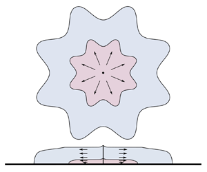
 $\rho _l$, spreading radially outwards over a rigid horizontal substrate, as depicted in the schematic of figure 1. The upper and lower layers are supplied at constant flux,
 $Q_0$ and
 $Q_{l0}$, respectively, at the origin. We denote physical quantities, such as the flux and viscosity, associated with the lower, lubricating later by the subscript
 $l$. We denote the surface heights of the upper and lower layers in the lubricated region by
 $z=H(r,\theta,t)$ and
 $z=h(r,\theta,t)$, respectively, where
 $r$ and
 $\theta$ are the radial and azimuthal coordinates, respectively. We also assume that there is no surface tension between the layers, and consider the limit in which vertical shear provides the dominant resistance to the flow of both layers.
Schematic of the flow of two superposed thin films of power-law viscous fluids spreading radially outwards under gravity over a horizontal substrate. Adapted from Part 1.

We assume a power-law non-Newtonian rheology for both films of fluid, so that the dynamic viscosities are given by
 \begin{equation} \mu = \tilde \mu \left|\frac{\partial \boldsymbol{u}}{\partial z}\right|^{{1}/{n}-1}, \quad \mu_l = \tilde \mu_l \left|\frac{\partial \boldsymbol{u}_l}{\partial z}\right|^{{1}/{n}-1}, \end{equation}
within the limits of lubrication theory, where  $\tilde \mu$ and
 $\tilde \mu _l$ are constant consistencies. As discussed in Part 1, the equal power-law exponents imply the existence of a self-similar axisymmetric flow. These flows have been examined in Part 1, including their dependence on the underlying dimensionless parameters
 \begin{equation} \mathcal{D} = \frac{\rho_l-\rho}{\rho}, \quad \mathcal{M} = \frac{\tilde \mu}{\tilde \mu_l}, \quad \mathcal{Q} = \frac{Q_{l0}}{Q_{0}}, \end{equation}
describing the density difference, consistency ratio and source flux ratio, respectively.
The flow considered in this paper is governed by a generalisation of the governing equations for axisymmetric flows developed in Part 1, to include non-axisymmetric disturbances. The governing equations and boundary conditions of § 2 of Part 1, apart from the expressions for the velocities and fluxes, are appropriate to examine such flows. To derive expressions for the velocities and fluxes, we begin by considering disturbances of order  $\epsilon \ll 1$ so that
 \begin{equation} \boldsymbol\phi=\boldsymbol{\phi}_0+\epsilon \boldsymbol{\phi}_1, \end{equation}
where  $\boldsymbol \phi =(h,H,\boldsymbol u, \boldsymbol u_l, \boldsymbol q, \boldsymbol q_l)$ and
 $\boldsymbol \phi _i=(h_i,H_i,\boldsymbol u_i, \boldsymbol u_{li}, \boldsymbol q_i, \boldsymbol q_{li})$ for
 $i=1,2$, such that
 $\partial \boldsymbol {\phi }_0/\partial \theta =0$. Specifically,
 \begin{equation} h=h_0(r,t)+\epsilon\,h_1(r,\theta,t), \quad H=H_0(r,t)+\epsilon\,H_1(r,\theta,t) \end{equation}
and
 \begin{gather} \boldsymbol u = u_{0}(r,z,t)\,\boldsymbol{e}_r + \epsilon \left[u_{r1}(r,\theta, z,t)\,\boldsymbol{e}_r+u_{\theta1}(r,\theta, z,t)\,\boldsymbol{e}_\theta\right], \end{gather}
 \begin{gather}\boldsymbol u_l = u_{l0}(r,z,t)\,\boldsymbol{e}_r + \epsilon \left[u_{lr1}(r,\theta, z,t)\,\boldsymbol{e}_r+u_{l\theta1}(r,\theta, z,t)\,\boldsymbol{e}_\theta\right], \end{gather}
 \begin{gather}\boldsymbol q = q_{0}(r,t)\,\boldsymbol{e}_r + \epsilon \left[q_{r1}(r,\theta,t)\,\boldsymbol{e}_r+q_{\theta1}(r,\theta,t)\,\boldsymbol{e}_\theta\right], \end{gather}
 \begin{gather}\boldsymbol q_l = q_{l0}(r,t)\,\boldsymbol{e}_r + \epsilon \left[q_{lr1}(r,\theta,t)\,\boldsymbol{e}_r+q_{l\theta1}(r,\theta,t)\,\boldsymbol{e}_\theta\right], \end{gather}
where  $\boldsymbol {e}_r$ and
 $\boldsymbol {e}_\theta$ are the radial and azimuthal unit basis vectors, respectively.
In what follows, we use the convention that the  $_0$ and
 $_1$ subscripts denote quantities referring to the basic state and perturbations, respectively, and the
 $_r$ and
 $_\theta$ subscripts denote quantities referring to the
 $r$- and
 $\theta$-components of a vector. That is, any vector quantity
 $\boldsymbol p$ can be expressed in the form
 \begin{equation} \boldsymbol p= (p_{r0}\boldsymbol{e}_r + p_{\theta0}\boldsymbol{e}_\theta) + \epsilon(p_{r1}\boldsymbol{e}_r + p_{\theta1}\boldsymbol{e}_\theta). \end{equation}
For expressions for the zeroth-order quantities  $u_0$,
 $u_{l0}$,
 $q_0$ and
 $q_{l0}$ in terms of the zeroth-order surface heights
 $h_0$ and
 $H_0$ and their gradients, we refer the reader to Appendix A. These were derived in § 2 of Part 1. For convenience, these zeroth-order quantities are denoted by the variables
 $h$,
 $H$,
 $u$,
 $u_l$,
 $q$ and
 $q_l$, without the
 $_0$ subscript, in Part 1.
We derive expressions for the perturbations by returning to the horizontal force balance in the no-slip and lubricated regions.
2.1. No-slip region
Integrating the horizontal force balance
 \begin{equation} \frac{\partial}{\partial z}\left(\mu\,\frac{\partial \boldsymbol u}{\partial z}\right) = \rho g\, \boldsymbol{\nabla} H \end{equation}
in the no-slip region  $r_L< r< r_N$ results in the velocity field
 \begin{equation} \boldsymbol{u} =\frac{1}{n+1} \left(\frac{\rho g}{\tilde \mu}\right)^n (H^{n+1}-(H-z)^{n+1}) |\boldsymbol{\nabla} H|^{n-1} (-\boldsymbol{\nabla} H), \end{equation}
and corresponding depth-integrated flux
 \begin{equation} \boldsymbol{q} =\frac{1}{n+2} \left(\frac{\rho g}{\tilde \mu}\right)^n H^{n+2} |\boldsymbol{\nabla} H|^{n-1} (-\boldsymbol{\nabla} H), \end{equation}
which are of the same functional form as for axisymmetric flows, including the non-axisymmetric contributions. These agree with Kowal & Worster (Reference Kowal and Worster2015). Linearising gives rise to the components
 \begin{gather} q_{r1} ={-}\frac{1}{n+2} \left(\frac{\rho g}{\tilde\mu }\right)^n H_0^{n+1} \left| \frac{\partial H_0}{\partial r}\right|^{n-1}\left(nH_0\,\frac{\partial H_1}{\partial r}+ (n+2)\,\frac{\partial H_0}{\partial r}\,H_1\right), \end{gather}
 \begin{gather}q_{\theta1} ={-}\frac{1}{n+2}\left(\frac{\rho g}{\tilde\mu }\right)^n H_0^{n+2} \left| \frac{\partial H_0}{\partial r}\right|^{n-1}\frac{1}{r}\,\frac{\partial H_1}{\partial\theta}, \end{gather}
of the perturbations to the flux.
Mass conservation, at first order, is described by
 \begin{equation} \frac{\partial H_1}{\partial t} ={-} \frac{1}{r}\,\frac{\partial (rq_{r1})}{\partial r} - \frac{1}{r}\,\frac{\partial q_{\theta1}}{\partial \theta}, \end{equation}
within the no-slip region  $r_L< r< r_N$. We note that additional terms are required when transforming to similarity variables (2.42) to capture terms involving the base state flow owing to perturbations in the frontal position.
2.2. Lubricated region
Unlike single-layer flows for any value of  $n$, and lubricated flows for
 $n=1$, there are no closed-form expressions for the velocity and flux, which include non-axisymmetric contributions, unless linearised.
We proceed by starting from the horizontal force balance
 \begin{gather} \frac{\partial}{\partial z}\left(\mu\,\frac{\partial \boldsymbol u}{\partial z}\right) = \rho g \boldsymbol{\nabla} H, \quad h< z< H, \end{gather}
 \begin{gather} \frac{\partial}{\partial z}\left(\mu_l\,\frac{\partial \boldsymbol {u_l}}{\partial z}\right) = \rho g (\mathcal{D} \boldsymbol{\nabla} h+\boldsymbol{\nabla} H), \quad 0< z< h, \end{gather}
in the upper and lower layers, supplemented by the stress-free boundary condition at  $z=H$, continuity of velocity and shear stress at
 $z=h$, and the no-slip boundary condition at
 $z=0$.
For the upper layer, this can be integrated directly so that
 \begin{equation} \boldsymbol{u} ={-}\left(\frac{\rho g}{\tilde \mu}\right)^n \frac{1}{n+1}[(H-z)^{n+1}- (H-h)^{n+1}]|\boldsymbol{\nabla} H|^{n-1} (-\boldsymbol{\nabla} H) + \boldsymbol u_I, \end{equation}
where  $\boldsymbol u_I$ is the interfacial velocity, to be determined by matching with the velocity of the lower layer. Linearising gives rise to the perturbed velocity
 \begin{align} \boldsymbol{u}_1
&={-}\left(\frac{\rho g}{\tilde \mu}\right)^n \frac{1}{n+1}
[[(H_0-z)^{n+1}-
(H_0-h_0)^{n+1}]|\boldsymbol{\nabla} H_0|^{n-1}
(-\boldsymbol{\nabla} H_1)\nonumber\\ &\quad +
(n-1)[(H_0-z)^{n+1}-
(H_0-h_0)^{n+1}]|\boldsymbol{\nabla}
H_0|^{n-3}(\boldsymbol{\nabla}
H_1\boldsymbol{\cdot}\boldsymbol{\nabla} H_0)
(-\boldsymbol{\nabla} H_0) \nonumber\\
&\quad{}+(n+1)[H_1(H_0-z)^n -
(H_1-h_1)(H_0-h_0)^n|\boldsymbol{\nabla} H_0|^{n-1}
(-\boldsymbol{\nabla} H_0)]] + \boldsymbol
u_{I1}, \end{align}
where  $\boldsymbol u_{I1}$ is the perturbed part of the interfacial velocity
 $\boldsymbol u_{I}$.
For the lower layer, we obtain
 \begin{equation} \frac{\partial\boldsymbol{u_l}}{\partial z} = \lvert\boldsymbol{a}-z\boldsymbol{c}\rvert^{n-1}(\boldsymbol{a}-z\boldsymbol{c}), \end{equation}
where
 \begin{gather} \boldsymbol{a} ={-}\frac{\rho g}{\tilde{\mu}}\,\mathcal{M}\left(H\boldsymbol{\nabla} H+\mathcal{D}h\boldsymbol{\nabla} h\right), \end{gather}
 \begin{gather} \boldsymbol{c} ={-}\frac{\rho g}{\tilde{\mu}}\,\mathcal{M}\left(\boldsymbol{\nabla} H+\mathcal{D}\boldsymbol{\nabla} h\right). \end{gather}
Linearising in  $\epsilon$ and integrating the linearised expressions yields
 \begin{align} u_{lr1} &= \frac{1}{(n+1)
c_{{r0}}^2} [(c_{{r1}} \left(a_{{r0}}+n z
c_{{r0}}\right)-(n+1) a_{{r1}} c_{{r0}}) \left|
a_{{r0}}-z c_{{r0}}\right| {}^{n-1} \left(a_{{r0}}-z
c_{{r0}}\right)\nonumber\\ &\quad+\left((n+1)
a_{{r1}} c_{{r0}}-a_{{r0}} c_{{r1}}\right) \left|
a_{{r0}}\right| {}^{n-1}a_{{r0}} ],
\end{align}
 \begin{align} u_{l\theta1} &=\frac{1}{n
(n+1) c_{{r0}}^2} [ \left(c_{{\theta 1}}
\left(a_{{r0}}+n z c_{{r0}}\right)-(n+1) a_{{\theta 1}}
c_{{r0}}\right) \left| a_{{r0}}-z c_{{r0}}\right| {}^{n-1}
\left(a_{{r0}}-z c_{{r0}}\right)\nonumber\\ &\quad +
\left((n+1) a_{{\theta 1}} c_{{r0}}-a_{{r0}} c_{{\theta
1}}\right) \left| a_{{r0}}\right| {}^{n-1} a_{{r0}} ], \end{align}
from which the interfacial velocity  $\boldsymbol {u_I}$ can be deduced. Explicitly,
 \begin{equation} \boldsymbol{u_I}= u_{I0}\boldsymbol{e_r}+\epsilon( u_{Ir1}\boldsymbol{e_r}+ u_{I\theta1}\boldsymbol{e_\theta}), \end{equation}
where
 \begin{gather} u_{I0}= \frac{1}{n+1}\left(\frac{\rho g}{\tilde \mu_l}\right)^{n} \frac{1}{\mathcal{D}\,\partial h_{0}/\partial r+\partial H_0/\partial r}\left[ \left|(H_0-h_0)\,\frac{\partial H_0}{\partial r}\right|^{n+1} \right.\nonumber\\ \hspace{12pt}\left. - \left|h_0\left(\mathcal{D}\,\frac{\partial h_0}{\partial r}+\frac{\partial H_0}{\partial r}\right)+(H_0-h_0)\,\frac{\partial H_0}{\partial r}\right|^{n+1} \right], \end{gather}
 \begin{gather} u_{Ir1}= \left[h_1\,\frac{\partial u_{lr0}}{\partial z}+u_{lr1}\right]_{z=h_0}, \end{gather}
 \begin{gather} u_{I\theta1}= \left[h_1\,\frac{\partial u_{l\theta0}}{\partial z}+u_{l\theta1}\right]_{z=h_0}. \end{gather}
Note that since the basic state is axisymmetric, it follows that  $a_{\theta 0}=c_{\theta 0}=0$. Expressions for
 $a_{r0}, a_{r1}, a_{\theta 1}, c_{r0}, c_{r1}$ and
 $c_{\theta 1}$ are specified explicitly in Appendix B.
Further integration yields the following expressions for the  $r$-components,
 \begin{gather} q_{lr1} = A_1h_1+A_2a_{r1}+A_3c_{r1}, \end{gather}
 \begin{gather} q_{r1} = A_4\,\frac{\partial H_1}{\partial r}+ A_5H_1+ A_6h_1+A_7a_{r1}+A_8c_{r1}, \end{gather}
and the  $\theta$-components,
 \begin{gather} q_{l\theta1} = A_9a_{\theta1}+A_{10}c_{\theta1}, \end{gather}
 \begin{gather} q_{\theta1} = A_{11}\,\frac{1}{r}\,\frac{\partial H_1}{\partial\theta}+ A_{12}a_{\theta1}+A_{13}c_{\theta1}, \end{gather}
of the perturbations to the fluxes of the two layers in the lubricated region, where the  $A_i$ are specified in Appendix B. These expressions reduce to those of Kowal & Worster (Reference Kowal and Worster2019b) for
 $n=1$.
Mass conservation, at first order in  $\epsilon$, is described by
 \begin{equation} \frac{\partial h_1}{\partial t} ={-} \frac{1}{r}\,\frac{\partial (rq_{lr1})}{\partial r} - \frac{1}{r}\,\frac{\partial q_{l\theta1}}{\partial \theta} \end{equation}
for the lower layer, and
 \begin{equation} \frac{\partial (H_1-h_1)}{\partial t} ={-} \frac{1}{r}\,\frac{\partial (rq_{r1})}{\partial r} - \frac{1}{r}\,\frac{\partial q_{\theta1}}{\partial \theta} \end{equation}
for the upper layer within the lubricated region  $0< r< r_L$. Similarly to the no-slip region, additional terms are required when transforming to similarity variables (2.41) to capture terms involving the base state flow owing to perturbations in the frontal position.
2.3. Boundary conditions
We apply the source flux conditions
 \begin{equation} \lim_{r\to0} 2{\rm \pi} r q_{lr} = Q_{l0}, \quad \lim_{r\to0} 2{\rm \pi} r q_{r} = Q_{0}, \end{equation}
the thickness and height continuity conditions
 \begin{equation} [H]^+_-= 0 \quad \text{and} \quad [(\boldsymbol{q}+\boldsymbol{q}_l)\boldsymbol\cdot \boldsymbol{n_L}]^+= [\boldsymbol{q}\boldsymbol{\cdot} \boldsymbol{n_L}]^- \quad (r=r_L), \end{equation}
where  $\boldsymbol {n_L}=\boldsymbol {e}_r -\boldsymbol {e}_\theta ({1}/{r_L})\,{\partial r_L}/{\partial \theta }+ {O}(\epsilon ^2)$ is an outward normal vector at the lubrication front, and the kinematic conditions
 \begin{equation} \dot r_L = \lim_{r\to r_L} \left.\left[ q_{lr} - q_{l\theta}\,\frac{1}{r_L}\,\frac{\partial r_L}{\partial \theta}\right] \right/h, \end{equation}
for the lubrication front and
 \begin{equation} \dot r_N = \lim_{r\to r_N} \left.\left[ q_{r} - q_{\theta}\,\frac{1}{r_N}\,\frac{\partial r_N}{\partial \theta}\right] \right/H, \end{equation}
for the leading edge. We also apply the zero-flux condition
 \begin{equation} \boldsymbol{q_l}\boldsymbol{\cdot} \boldsymbol{n_L} = 0 \quad (r=r_L) \end{equation}
at the lubrication front for  $\mathcal {D}\neq 0$, and
 \begin{equation} \boldsymbol{q}\boldsymbol{\cdot} \boldsymbol{n_N}=0\quad (r=r_N) \end{equation}
at the leading edge, where  $\boldsymbol {n_N}=\boldsymbol {e}_r -\boldsymbol {e}_\theta ({1}/{r_N})\,{\partial r_N}/{\partial \theta }+ {O}(\epsilon ^2)$ is an outward normal vector at the leading edge.
2.4. Similarity coordinates
To conduct a linear stability analysis about the self-similar axisymmetric flow of Part 1, we revert to the similarity coordinates  $(\xi, \phi, \tau )$ defined by
 \begin{gather} r=\left(\frac{\rho g}{\tilde \mu}\right)^\alpha t^\beta Q_0^\gamma \xi\xi_L ,\quad \text{for} 0< r< r_L, \end{gather}
 \begin{gather}r=\left(\frac{\rho g}{\tilde \mu}\right)^\alpha t^\beta Q_0^\gamma [\xi_L+(\xi-1)(\xi_N-\xi_L)], \quad \text{for} \ r_L< r< r_N, \end{gather}
 \begin{gather}\tau=\log t, \quad \phi=\theta. \end{gather}
where  $0<\xi <1$ corresponds to the lubricated region
 $0< r< r_L$, and
 $1<\xi <2$ corresponds to the no-slip region
 $r_L< r< r_N$. The constants
 $\alpha$,
 $\beta$ and
 $\gamma$ are given by
 \begin{equation} \alpha =\frac{n}{5n+3}, \quad \beta = \frac{2n+2}{5n+3}, \quad \gamma=\frac{2n+1}{5n+3}, \end{equation}
as specified in Part 1.
The lubricated region is therefore mapped to the interval  $(0,1)$, and the no-slip region is mapped to the interval
 $(1,2)$. Perturbations to the two fronts can be read from
 \begin{align} \xi_L(\phi,\tau) = \xi_{L0}+\epsilon \xi_{L1}\exp({\sigma \tau+{\rm i}k\phi}), \quad \xi_N(\phi,\tau) = \xi_{N0}+\epsilon \xi_{N1}\exp({\sigma \tau+{\rm i}k\phi}), \end{align}
in similarity coordinates. Here,  $\xi _{L0}$ and
 $\xi _{N0}$ correspond to the unperturbed positions of the intrusion front and leading edge, respectively. Both
 $\xi _{L0}$ and
 $\xi _{N0}$ are constants. We are searching for normal mode solutions of growth rate
 $\sigma$ and azimuthal wavenumber
 $k$, which exist under the change of variables (2.41)–(2.43a,b). Under this transformation, contributions owing to the perturbations to the two frontal positions are reflected through appropriate terms in the governing equations, rather than through the boundary conditions. Such an approach eliminates difficulties associated with the stress singularities at the two fronts.
The zeroth- and first-order surface heights are transformed as
 \begin{equation} \left(\begin{array}{@{}c@{}}
h_0(r,t)\\H_0(r,t)\\h_1(r,\theta,t)\\H_1(r,\theta,t)
\end{array}\right) = \left(\frac{\rho g}{\tilde
\mu}\right)^at^bQ_0^c\boldsymbol{\cdot}
\left(\begin{array}{@{}c@{}}f_0(\xi)\\F_0(\xi)\\f_1(\xi)
\exp({\sigma \tau+{\rm i}k\phi})\\F_1(\xi) \exp({\sigma
\tau+{\rm i}k\phi})\end{array}\right),
\end{equation}
and the components of the flux of the two layers are transformed as
 \begin{equation} \left( \begin{array}{@{}c@{}} q_{lr0}(r,t)\\ q_{r0}(r,t) \end{array} \right) = \left(\frac{\rho g}{\tilde \mu}\right)^{-\alpha}t^{-\beta}Q_0^{1-\gamma} \left( \begin{array}{@{}c@{}} \tilde q_{lr0}(\xi)\\ \tilde q_{r0}(\xi) \end{array} \right) \end{equation}
at zeroth order, and
 \begin{equation} \left(\begin{array}{@{}c@{}} q_{lr1}(r,\theta,t)\\ q_{l\theta1}(r,\theta,t)\\ q_{r1}(r,\theta,t)\\ q_{\theta1}(r,\theta,t) \end{array} \right)= \left(\frac{\rho g}{\tilde \mu}\right)^{-\alpha}t^{-\beta}Q_0^{1-\gamma} \exp({\sigma \tau+{\rm i}k\phi}) \left( \begin{array}{@{}c@{}} \tilde q_{lr1}(\xi)\\ \tilde q_{l\theta1}(\xi)\\ \tilde q_{r1}(\xi)\\ \tilde q_{\theta1}(\xi) \end{array} \right) \end{equation}
at first order, where the constants  $a$,
 $b$ and
 $c$ are given by
 \begin{equation} a={-}\frac{2n}{5n+3}, \quad b=\frac{n-1}{5n+3}, \quad c=\frac{n+1}{5n+3}, \end{equation}
as functions of  $n$.
Correspondingly, after dropping tildes for convenience, the components of the flux perturbations are given by the expressions
 \begin{gather} q_{lr1}=B_1 f_1'+B_2 F_1'+B_3 f_1+B_4 F_1+B_5 \xi _{{L1}}, \end{gather}
 \begin{gather} q_{l\theta 1}={\rm i}k (B_6 f_1 + B_7 F_1), \end{gather}
for the lower layer, and
 \begin{gather} q_{r1} = B_8 f_1'+B_9 F_1'+B_{10} f_1+B_{11} F_1+B_{12} \xi _{{L1}}, \end{gather}
 \begin{gather} q_{\theta 1} = {\rm i}k(B_{13} f_1+B_{14} F_1) -{\rm i}k\xi\,\frac{\xi_{L1}}{\xi_{L0}}\,(B_{13} f_0'+B_{14} F_0'), \end{gather}
for the upper layer. In the no-slip region, the components become
 \begin{gather} q_{r1} = B_{15}F_1'+B_{16}F_1 + B_{17} \left(\xi _{{N1}}-\xi _{{L1}}\right), \end{gather}
 \begin{gather} q_{\theta 1} = {\rm i}kB_{18}\left((\xi_{L0}-\xi_{N0}) F_1 + \xi_{{N1}}(\xi-1) F_0' - \xi_{{L1}}(\xi-2)F_0' \right), \end{gather}
where the  $B_i$ are specified in Appendix B. These expressions reduce to those of Kowal & Worster (Reference Kowal and Worster2019b) for
 $n=1$.
The mass conservation equations become
 \begin{equation} \left(\sigma+\frac{n -1}{5 n+3}\right)f_1 -\frac{2 (n+1)}{5 n+3}\,\xi f_1' -\frac{ \sigma \xi _{L1}}{\xi _{{L0}}}\,\xi f_0' ={-}\frac{ (\xi q_{{lr1}})' +{\rm i} k q_{{l\theta1}} }{\xi \xi _{{L0}}} + \frac{ \xi _{L1} \left(\xi q_{{lr0}}\right)'}{\xi \xi _{{L0}}^2} \end{equation}
for the lower layer of the lubricated region, and
 $$\begin{gather} \left(\sigma+\frac{n -1}{5 n+3}\right)(F_1-f_1) -\frac{2 (n+1)}{5 n+3}\,\xi (F_1'-f_1') -\frac{ \sigma \xi _{L1}}{\xi _{{L0}}}\,\xi (F_0'-f_0')\nonumber\\ ={-}\frac{ (\xi q_{{r1}})' +{\rm i} k q_{{\theta1}} }{\xi \xi _{{L0}}} + \frac{ \xi _{L1} \left(\xi q_{{r0}}\right)'}{\xi \xi _{{L0}}^2} \end{gather}$$
for the upper layer of the lubricated region. These include contributions owing to the perturbations to the frontal positions. The mass conservation equation in the no-slip region becomes
 $$\begin{gather} \left(\sigma+\frac{n -1}{5 n+3}\right) C_{1} F_1 - \frac{2(n+1)}{5 n+3}\,C_{2} F_1' - \frac{2(n+1)}{5 n+3}\,C_{3} F_0' + \sigma C_{4}F_0' \nonumber\\ =C_{5}(q_{{r1}}-{\rm i} k q_{{\theta1}}) +q_{{r1}}' +C_{6}q_{{r0}}' + C_{7}q_{r0}, \end{gather}$$
where the  $C_i$ are specified in Appendix B.
The source flux boundary conditions reduce to
 \begin{equation} \lim_{\xi\rightarrow0}2{\rm \pi}\xi(\xi_{L0} q_{lr1}+\xi_{L1} q_{lr0}) = 0, \quad \lim_{\xi\rightarrow0}2{\rm \pi}\xi(\xi_{L0} q_{r1}+\xi_{L1} q_{r0}) = 0, \end{equation}
and the matching conditions at the lubrication front reduce to
 \begin{gather} \left[ F_1 \right]^+_-= 0 \quad (\xi=1), \end{gather}
 \begin{gather} \left[ q_{r1} \right]^+_-= 0 \quad (\xi=1). \end{gather}
Note that contributions owing to the perturbations to the frontal positions do not appear in these matching conditions as they are built into the governing equations instead. The remaining boundary conditions are the zero flux conditions
 \begin{equation} q_{lr1} = 0 \quad (\xi=1) \end{equation}
at the lubrication front, and
 \begin{equation} q_{r1} = 0 \quad (\xi=2) \end{equation}
at the leading edge.
Note that the fronts are given by  $\xi =1$ and
 $\xi =2$ by the definition (2.41)–(2.42) of the scaled similarity coordinate, as
 $\xi _L$ and
 $\xi _N$ are scaled out. The perturbations to the front (from linearising
 $\xi _L=\xi _{L0}+\epsilon \xi _{L1}$ and
 $\xi _N=\xi _{N0}+\epsilon \xi _{N1}$) are factored into the governing equations, rather than the radial coordinate by scaling
 $\xi _L$ and
 $\xi _N$ out as in (2.41)–(2.42).
The kinematic conditions become
 \begin{equation} \frac{2n+2}{5n+3}\,(1+\sigma)\xi_{L1} = \lim_{\xi\to1} \left[ \frac{q_{lr1}}{f_0} - \frac{ q_{lr0}f_1}{f_0^2} \right] \end{equation}
at the lubrication front, and
 \begin{equation} \frac{2n+2}{5n+3}\,(1+\sigma)\xi_{N1} = \lim_{\xi\to2} \left[ \frac{q_{r1}}{F_0} - \frac{ q_{r0}F_1}{F_0^2} \right] \end{equation}
at the leading edge, which lead to the asymptotic solutions described in the following subsection.
3. Asymptotic solutions
3.1. Asymptotic solutions near the two fronts
An asymptotic analysis near the two fronts, in which the governing equations (2.56) and (2.58) are solved in an inner region by rescaling  $f_1=\delta ^p \hat f_1$,
 $F_1=\delta ^p \hat F_1$,
 $\xi =1-\delta X$ (near the intrusion front) and
 $\xi =2-\delta X$ (near the leading edge), and balancing dominant terms in the limit
 $\delta \ll 1$, gives rise to
 $p={n}/{(2n+1)}$ and the asymptotic solutions
 \begin{equation} f_1\sim \frac{(5 n\!+\!3) \sigma +2 (n\!+\!1)^2 }{(n+1) (2 n+1) } \left[\frac{(n+1) (n+2)}{5 n+3} \left(\frac{2 n+1}{4 n\mathcal{MD}\xi_{L0}}\right)^{n} \right]^{{1}/({2 n+1})} \xi_{L1}(1\!-\!\xi)^{{n}/({2n+1})}, \end{equation}
as  $\xi \to 1^-$, near the lubrication front, and
 \begin{equation} F_1\sim \mathcal{A}(2-\xi)^{{n}/({2n+1})}, \end{equation}
as  $\xi \to 2^-$, near the leading edge, where
 \begin{align} \mathcal{A}=\left(\frac{2 (n\!+\!1) (n\!+\!2)\xi_{N0} (\xi_{N0}\!-\!\xi_{L0})^n}{(5 n\!+\!3) (2 n\!+\!1)^{n+1}n^n }\right)^{{1}/({2 n\!+\!1})} \left[\frac{n (\xi_{N1}\!-\!\xi_{L1})}{\xi_{N0}\!-\!\xi_{L0}}+\frac{\xi_{N1}}{\xi_{N0}} \left(\frac{(5 n+3) \sigma }{2 (n+1)}+1\right)\right]. \end{align}
These asymptotic solutions are of the same spatial structure as those of the basic state, with prefactors proportional to a linear combination of the perturbations to the frontal positions. These reduce to the asymptotic solutions of Kowal & Worster (Reference Kowal and Worster2019b) in the limit  $n=1$. The asymptotic solutions are used to alleviate difficulties associated with the stress singularities that occur at the two fronts, when solving for the solutions numerically.
3.2. Transformation near the origin
An artefact of radially spreading lubricated viscous gravity currents, supplied at constant flux at the origin, is that the thickness of both layers of fluid approaches a point singularity at the origin, as a finite amount of fluid is being supplied from a single point. The form of the solutions, towards which the surface heights approach at zeroth order in  $\epsilon$, are specified in Part 1. The asymptotic behaviour is of different character depending on the value of
 $n$, specifically, depending on whether
 $n<1$,
 $n=1$ or
 $n>1$. A similar phenomenon occurs at first order, which we examine by rescaling
 $\xi =\delta X$,
 $f_1=\delta ^p \hat f_1$,
 $F_1=\delta ^p \hat F_1$ and balancing dominant terms of (2.56)–(2.57) in the limit
 $\delta \ll 1$.
For  $n<1$, the general solution for the perturbations to the surface heights
 $f_1$ and
 $F_1$ approaches the functional form
 $\xi ^\lambda$, where
 \begin{equation} \lambda=\lambda_{{\pm}} = \frac{1-n\pm(n+1) \sqrt{4 k^2 n +(n-1)^2}}{2 n (n+1)}. \end{equation}
For  $n>1$, the exponent is, instead, given by
 \begin{equation} \lambda=\lambda_{{\pm}} = \frac{n-1\pm\sqrt{4 k^2 n+(n-1)^2}}{2 n}. \end{equation}
The dominant term as  $\xi \to 0$ corresponds to
 $\lambda =\lambda _{-}$. In the limit
 $n\to 1$, approaching from either the left or the right, the power-law dependence of
 $f_1(\xi )$ and
 $F_1(\xi )$ is of the form
 $\xi ^{-k}$.
These exponents become large in magnitude for large  $k$, for any
 $n$. Therefore, to resolve this singularity at the origin for all wavenumbers and to ensure numerical stability, we reformulate the problem in terms of
 $g_1(\xi )=\xi ^{-\lambda _-}\,f_1(\xi )$ and
 $G_1(\xi )=\xi ^{-\lambda _-}\,F_1(\xi )$, instead of
 $f_1(\xi )$ and
 $F_1(\xi )$, and revert back to
 $f_1(\xi )$ and
 $F_1(\xi )$ through a change of variables after the governing equations have been solved numerically. Although it does not provide a formal asymptotic solution, this is useful in regularising numerical computations by providing a convenient choice for a scaling factor.
As described in Kowal & Worster (Reference Kowal and Worster2019b), for  $n=1$ we instead solve for
 \begin{equation} ( g_1 , G_1 ) = \xi^{k} ( - \log \xi)^{3/4} (f_1(\xi), F_1(\xi)). \end{equation}
The prefactor, similarly, involves an exponent that grows with  $k$.
4. Numerical method
We use a shooting method to solve the perturbation equations, by shooting backwards for  $\xi _{L1}$ and
 $\xi _{N1}$ from the nose
 $\xi =2$, and matching across the intrusion front
 $\xi =1$. The process is similar to that of Kowal & Worster (Reference Kowal and Worster2019b), except that distinction is made between
 $n<1$,
 $n=1$ and
 $n>1$. As the governing equations are singular at both tips,
 $\xi =1$ and
 $\xi =2$, we apply the asymptotic solution (3.2) to initiate the computations at
 $\xi =2-\delta$, where
 $\delta \ll 1$ is a small distance away from the singular tip. We integrate backwards towards the singularity at the intrusion front,
 $\xi =1^+$, and apply matching conditions and the asymptotic solution (3.1) at
 $\xi =1-\delta$, a small distance
 $\delta$ away from the singularity at the intrusion front. These are used to initiate computations in the lubricated region, which we solve numerically by integrating backwards towards
 $\xi =\varDelta$, where
 $\varDelta \ll 1$. As such, the problem is solved numerically on the subdomain
 $[\varDelta,1-\delta ]\cup [1,2-\delta ]$, to avoid numerical issues with singularities at both exterior boundaries
 $\xi =0$ and
 $\xi =2$, and the interior boundary
 $\xi =1$.
The governing equations pose an eigenvalue problem consisting of differential equations for  $f_1$ and
 $F_1$, or equivalently,
 $g_1$ and
 $G_1$. As explained in § 3.2, we solve for
 $g_1$ and
 $G_1$, instead of
 $f_1$ and
 $F_1$, for numerical stability at large wavenumbers. As the system is an eigenvalue problem, non-zero solutions exist only for specific growth rates, or eigenvalues,
 $\sigma$. We exploit the linearity of the system of governing equations to solve for the eigensolutions
 $\boldsymbol \varPsi (\xi )=(g_1(\xi ),\; G_1(\xi ),\; \xi _{L1}, \;\xi _{N1})$ and associated growth rate
 $\sigma$ iteratively. Owing to the order of the eigenvalue problem, this involves searching across two-dimensional parameter space for the appropriate values of
 $\xi _{L1}$ and
 $\xi _{N1}$. As such, for any wavenumber and physical parameter values, the iterative process begins with an initial estimate for
 $\sigma$, from which two linearly independent solutions for the perturbations are obtained numerically by shooting backwards. These two numerical solutions correspond to two perturbation problems, Problems
 $a$ and
 $b$ are defined by the values of
 $\xi _{L1}$ and
 $\xi _{N1}$. Specifically, Problem
 $a$ is defined by setting
 $\xi _{L1} = 1$ and
 $\xi _{N1} = 0$, giving rise to a numerical solution
 $\boldsymbol \varPsi _a$, whereas Problem
 $b$ is defined by setting
 $\xi _{L1} = 0$ and
 $\xi _{N1} = 1$, giving rise to a numerical solution
 $\boldsymbol \varPsi _b$. The set
 $\{\boldsymbol \varPsi _a, \; \boldsymbol \varPsi _b\}$ forms two non-zero linearly independent solutions satisfying the perturbation equations and all the boundary and matching conditions apart from the source flux conditions, which we apply at
 $\xi =\varDelta$, that is,
 \begin{equation} 2{\rm \pi}\xi(\xi_{L0} q_{lr1}+\xi_{L1} q_{lr0}) = 0, \quad 2{\rm \pi}\xi(\xi_{L0} q_{r1}+\xi_{L1} q_{r0}) = 0 \quad (\xi=\varDelta). \end{equation}
By linearity of the governing equations, any linear combination of the solutions  $\boldsymbol \varPsi _a$ and
 $\boldsymbol \varPsi _b$ is also a solution of the perturbation equations and all the boundary and matching conditions, apart, in general, from the source flux conditions. It is our aim to select a linear combination for which the source flux conditions are also satisfied. Such a linear combination is the desired numerical solution to the perturbation equations. To select it, we define the residual matrix
 \begin{equation} \boldsymbol R = 2{\rm \pi} \varDelta \left.\left( \begin{array}{@{}cc@{}} \xi_{L0}q^a_{l1r} + \xi_{L1}q^a_{l0r} & \xi_{L0}q^b_{l1r} + \xi_{L1}q^b_{l0r} \\[3pt] \xi_{L0}q^a_{1r} + \xi_{L1}q^a_{0r} & \xi_{L0}q^b + \xi_{L1}q^b \end{array} \right)\right|_{\xi=\varDelta}, \end{equation}
the columns of which measure the residual in the source flux vectors, corresponding to Problems  $a$ and
 $b$, respectively. The desired solution is one for which the determinant of the residual matrix vanishes, indicating that there exists a linear combination of the two test solutions for which the two source flux boundary conditions are satisfied. We use a root finder to find a growth rate
 $\sigma$ for which the determinant of the residual matrix is close to zero, within a specified tolerance. This is a one-dimensional root-finding problem, for which the determinant of the residual matrix is used to update
 $\sigma$ at each iteration, as described in Kowal & Worster (Reference Kowal and Worster2019b).
As this process yields more than one eigenvalue  $\sigma$, we are interested in the eigensolution for which
 $\sigma$ is largest, which corresponds physically to the maximal growth rate for a given wavenumber. Once the largest growth rate is found for a given set of physical parameter values, we employ parameter continuation to determine growth rates across parameter space.
We note that the problem is  $2{\rm \pi}$-periodic in
 $\theta$, and as such, only integer multiples of
 $k$ are admissible. In all plots that follow, the results are interpolated for non-integer values of
 $k$.
Neutral curves for  $\mathcal {M}$ as a function of
 $k$ for
 $\mathcal {D}=2$,
 $\mathcal {Q}=0.1$ and various values of
 $n$. The inset shows the critical consistency ratio
 $\mathcal {M}_c$ as a function of
 $n$.

5. Discussion of results
As in the Newtonian limit, a necessary condition for the onset of instability can be understood by considering a balance of fluxes either side of the intrusion front. In the  $\mathcal {D}=0$ limit, a combination of the flux and height continuity conditions gives
 \begin{equation} (\mathcal{M}^n-1) \left[ 1- \left(1-\frac{f_0}{F_0}\right)^{n+2} \right] \left[ \left|\frac{{\rm d} F_0}{{\rm d}R}\right|^{n-1} \frac{{\rm d} F_0}{{\rm d}R}\right]^-{=} \left[ \left|\frac{{\rm d} F_0}{{\rm d}R}\right|^{n-1} \frac{{\rm d} F_0}{{\rm d}R} \right]^+_-, \end{equation}
where  $R=\xi _L\xi$ for
 $\xi <1$, and
 $R=\xi _L+(\xi _N-\xi _L)(\xi -1)$ for
 $1<\xi <2$. Noting that
 $q_{lr0}+q_{r0}>0$,
 $F_0>f_0$ and
 \begin{equation} q_{lr0}+q_{r0}={-}\frac{1}{n+2} \left[ (F_0-f_0)^{n+2} + \mathcal{M}^n\left(F_0^{n+2} - (F_0-f_0)^{n+2} \right) \right]\left|\frac{{\rm d} F_0}{{\rm d}R}\right|^{n-1} \frac{{\rm d} F_0}{{\rm d}R}, \end{equation}
it follows that  ${\rm d}F_0/{\rm d}R<0$. Therefore,
 \begin{equation} \left[ \left|\frac{{\rm d} F_0}{{\rm d}R}\right|^{n-1} \frac{{\rm d} F_0}{{\rm d}R} \right]^+_-{>}0 \end{equation}
if  $\mathcal {M}>1$. That is, there is a positive jump in a transformed pressure gradient across the lubrication front if the intruding fluid is less viscous. As seen in figure 2,
 $\mathcal {M}>1$, and hence (5.3), a necessary condition for instability to occur for the range of
 $n$ considered.
More precise specifications for when the flow is unstable can be obtained by solving the full eigenvalue problem numerically. Representative growth rates for typical parameter values versus the wavenumber are shown in figure 3 for a range of power-law exponents  $n$, where it can be seen that increasing power-law exponents promote instability. Surface plots of the growth rates across parameter space for a representative shear-thinning and shear-thickening case are shown in figures 4 and 5. Growth rates increase with
 $k$ for low wavenumbers, and decrease with
 $k$ for high wavenumbers, with an interval of unstable wavenumbers that is bounded from below and from above. Neutral curves for the consistency ratio
 $\mathcal {M}$, density difference
 $\mathcal {D}$ and flux ratio
 $\mathcal {Q}$, depicting the range of unstable wavenumbers, are shown in figures 2, 6 and 7, respectively. Instability occurs for large enough consistency ratios and low enough density differences. Physically, the larger the consistency ratio, the greater the jump in hydrostatic pressure gradient across the lubrication front, which promotes instability. However, the larger the density difference, the greater the influence of the buoyancy forces associated with the spreading of the lower layer near its nose, which is stabilising.
Growth rates  $\sigma$ versus the wavenumber
 $k$ for
 $\mathcal {M}=5$,
 $\mathcal {D}=2$,
 $\mathcal {Q}=0.1$ and various values of
 $n$.

Growth rates as a function of  $k$ and
 $\mathcal {M}$ for
 $\mathcal {D}=2$,
 $\mathcal {Q}=0.1$ and (a)
 $n=0.8$, (b)
 $n=1.2$. The
 $\sigma =0$ contour is drawn as a thick dashed red curve.

Growth rates as a function of  $k$ and
 $\mathcal {D}$ for
 $\mathcal {M}=10$,
 $\mathcal {Q}=0.1$ and (a)
 $n=0.8$, (b)
 $n=1.2$. The
 $\sigma =0$ contours are drawn as thick dashed red curves.

The regions of instability expand for increasing exponents  $n$. For each value of
 $n$, the system is unstable below a critical density difference
 $\mathcal {D}_c$ (defined as the maximum of the neutral curve for
 $\mathcal {D}$, plotted in the inset of figure 6) within a bounded window of wavenumbers. Small changes in the density difference, below its critical value, lead to small (large) changes to the interval of unstable wavenumbers when
 $n>1$ (
 $n<1$). On the other hand, small changes in the consistency ratio, above its critical value
 $\mathcal {M}_c$ (defined as the minimum of the neutral curve for
 $\mathcal {M}$, plotted in the inset of figure 2), lead to large (small) changes to the interval of unstable wavenumbers when
 $n>1$ (
 $n<1$). Instabilities occur only for large enough wavenumbers above a given threshold at a given flux ratio, and this threshold decreases with
 $n$ as seen in figure 7. This can also be seen in figure 8, which shows the neutral curve for
 $n$ versus
 $k$. Increasing values of
 $n$ permit a larger range of unstable wavenumbers
 $k$. Changes in
 $n$ are less significant for
 $n>1$ than for
 $n<1$. The slope of the neutral curve for
 $n$ is much lower for
 $n<1$ than for
 $n>1$.
Neutral curves for  $\mathcal {D}$ as a function of
 $k$ for
 $\mathcal {M}=10$,
 $\mathcal {Q}=0.1$ and various values of
 $n$.

Neutral curves for  $\mathcal {Q}$ as a function of
 $k$ for
 $\mathcal {M}=10$,
 $\mathcal {D}=2$ and various values of
 $n$.

Neutral curve for  $n$ as a function of
 $k$ for
 $\mathcal {M}=5$,
 $\mathcal {Q}=0.1$,
 $\mathcal {D}=1$.

The critical wavenumber  $k_c$ corresponding to the maximal growth rate
 $\sigma _c$ is shown in figure 9 as it varies with
 $n$. The maximal growth rate is positive only for large enough
 $n$, and both the critical wavenumber and the associated growth rate increase with
 $n$. Shear-thinning, in general, promotes instability, and the selected number of fingers increases the more shear-thinning the rheology.
(a) Critical wavenumber  $k_c$, and (b) associated growth rate
 $\sigma _c$, versus
 $n$, for
 $\mathcal {M}=5$,
 $\mathcal {D}=2$,
 $\mathcal {Q}=0.1$. The values of
 $k_c$ and
 $\sigma _c$ for
 $\sigma _c<0$ are dashed.

6. Conclusions
We have investigated the role of shear-thinning and shear-thickening on viscous fingering instabilities that occur within lubricated viscous gravity currents. The results are an extension of, and agree with, the stability analysis of Kowal & Worster (Reference Kowal and Worster2019b) in the Newtonian limit.
These instabilities are driven by a jump in hydrostatic pressure gradient across the intrusion front, which is found to be more pronounced the higher the consistency ratio between the two viscous fluids. As such, instabilities occur only for high enough consistency ratios. These instabilities, in turn, are stabilised by buoyancy forces associated with the lower layer near its nose, which become dominant for high density differences between the two layers. As such, the instabilities occur only for low enough density differences. The instability is suppressed completely above a critical density difference and below a critical consistency ratio.
These behaviours are maintained for all power-law exponents. However, the instability thresholds, as well as the preferred number of fingers, are altered. Specifically, shear-thinning promotes instability, and the system selects a greater number of fingers the more shear-thinning the rheology. The critical consistency ratio, above which instabilities occur, decreases the more shear-thinning the rheology. Although the interval of unstable wavenumbers is large (small) close to the critical value of the consistency ratio the more shear-thinning (shear-thickening) the rheology, the system tends to select large wavenumbers as the preferred mode of instability the more shear-thinning the rheology. As such, a large variation in the number of fingers may be expected close to the critical value of the consistency ratio in experiments. In contrast, the interval of unstable wavenumbers is small (large) the more shear-thinning (shear-thickening) the rheology when the density difference is close to its critical value. This leads to a smaller variation in the number of fingers that can be expected to be seen in experiments close to the critical value of the density difference.
Funding
L.T.L. acknowledges the support of a summer studentship through the Trinity College Summer Studentship Scheme. K.N.K. acknowledges funding through L'Oréal-UNESCO UK and Ireland, For Women In Science (FWIS).
Data availability statement
The data that support the findings of this study are available directly within this publication.
Declaration of interests
The authors report no conflict of interest.
Appendix A. Basic state velocities and fluxes
As obtained in Part 1, the basic state velocity is given by
 \begin{align} u_0&= \frac{1}{n+1}\left(\frac{\rho g}{\tilde \mu_l}\right)^{n} \frac{1}{\mathcal{D}\,\partial h_{0}/\partial r+\partial H_0/\partial r}\left[ \left|(H_0-h_0)\,\frac{\partial H_0}{\partial r}\right|^{n+1}\right. \nonumber\\ &\left.\quad -\left|h_0\left(\mathcal{D}\,\frac{\partial h_0}{\partial r}+\frac{\partial H_0}{\partial r}\right)+(H_0-h_0)\,\frac{\partial H_0}{\partial r}\right|^{n+1} \right] \nonumber\\ &\quad +\frac{1}{n+1}\left(\frac{\rho g}{\tilde \mu}\right)^n \left[(H_0-z)^{n+1} - (H_0-h_0)^{n+1}\right] \left|\frac{\partial H_0}{\partial r}\right|^{n-1} \frac{\partial H_0}{\partial r} \end{align}
for the upper layer, and
 $$\begin{align} u_l&=\frac{1}{n+1}\left(\frac{\rho g}{\tilde \mu_l}\right)^{n} \frac{1}{\mathcal{D}\,\partial h_0/\partial r+\partial H_0/\partial r} \left[ \left|(h_0-z)\left(\mathcal{D}\,\frac{\partial h_0}{\partial r}+\frac{\partial H_0}{\partial r}\right)+(H_0-h_0)\,\frac{\partial H_0}{\partial r}\right|^{n+1}\right. \nonumber\\ &\quad - \left. \left|h_0\left(\mathcal{D}\,\frac{\partial h_0}{\partial r}+\frac{\partial H_0}{\partial r}\right)+(H_0-h_0)\,\frac{\partial H_0}{\partial r}\right|^{n+1} \right] \end{align}$$
for the lower layer.
The corresponding depth-integrated line fluxes are given by
 \begin{align} q&= \frac{1}{n+1}\left(\frac{\rho g \mathcal{M}}{\tilde \mu}\right)^{n} \frac{H_0-h_0}{\mathcal{D}\,{\partial h_0}/{\partial r}+{\partial H_0}/{\partial r}} \left[ \left|(H_0-h_0)\,\frac{\partial H_0}{\partial r}\right|^{n+1}\right. \nonumber\\ &\left.\quad - \left|h\left(\mathcal{D}\,\frac{\partial h_0}{\partial r}+\frac{\partial H_0}{\partial r}\right) +(H_0-h_0)\,\frac{\partial H_0}{\partial r}\right|^{n+1} \right] \nonumber\\ &\quad -\frac{1}{n+2} \left(\frac{\rho g}{\tilde \mu}\right)^n (H_0-h_0)^{n+2} \left|\frac{\partial H_0}{\partial r}\right|^{n-1}\frac{\partial H_0}{\partial r} \end{align}
for the upper layer, and
 \begin{align} q_l &=
\frac{1}{n+1}\left(\frac{\rho g\mathcal{M}}{\tilde
\mu}\right)^{n} \frac{1}{\mathcal{D}\,\partial h_0/\partial
r+\partial H_0/\partial r}\left[
-\frac{1}{n+2}\,\frac{1}{\mathcal{D}\,{\partial
h_0}/{\partial r}+{\partial H_0}/{\partial
r}}\right.\nonumber\\ &\quad{}\times\left[
\left|(H_0-h_0)\,\frac{\partial H_0}{\partial
r}\right|^{n+1} (H_0-h_0)\,\frac{\partial H_0}{\partial
r}-\left|h_0\left(\mathcal{D}\,\frac{\partial h_0}{\partial
r}+\frac{\partial H_0}{\partial r}\right)\right.\right.
\nonumber\\ &\left.\left.\quad+(H_0-h_0)\,\frac{\partial
H_0}{\partial
r}\right|^{n+1}\left(h_0\left(\mathcal{D}\,\frac{\partial
h_0}{\partial r}+\frac{\partial H_0}{\partial
r}\right)+(H_0-h_0)\,\frac{\partial H_0}{\partial r}\right)
\right]\nonumber\\
&\left.\quad-h_0\left|h_0\left(\mathcal{D}\,\frac{\partial
h_0}{\partial r}+\frac{\partial H_0}{\partial
r}\right)+(H_0-h_0)\,\frac{\partial H_0}{\partial
r}\right|^{n+1} \right] \end{align}
for the lower layer.
Appendix B. Quantities appearing throughout the analysis
B.1. Quantities describing the perturbed dimensional flux
The following quantities are used to formulate expressions for the dimensional velocity and flux of either layer of the lubricated region:
 $$\begin{gather} c_{r0}(r,t) ={-}\frac{ \rho g \mathcal{M}}{\tilde\mu }\left(\mathcal{D}\,\frac{\partial h_0}{\partial r}+ \frac{\partial H_0}{\partial r}\right), \end{gather}$$
 $$\begin{gather}c_{r1}(r,\theta,t)={-}\frac{ \rho g \mathcal{M}}{\tilde\mu }\left(\mathcal{D}\,\frac{\partial h_1}{\partial r}+\frac{\partial H_1}{\partial r}\right), \end{gather}$$
 $$\begin{gather}c_{\theta1}(r,\theta,t)={-}\frac{ \rho g \mathcal{M}}{\tilde\mu }\left(\mathcal{D}\, \frac{1}{r}\,\frac{\partial h_1}{\partial \theta}+\frac{1}{r}\,\frac{\partial H_1}{\partial \theta}\right), \end{gather}$$
 $$\begin{gather}a_{r0}(r,t)={-}\frac{ \rho g \mathcal{M}}{\tilde\mu }\left(\mathcal{D}h_0\,\frac{\partial h_0}{\partial r} +H_0\,\frac{\partial H_0}{\partial r}\right), \end{gather}$$
 $$\begin{gather}a_{r1}(r,\theta,t)={-}\frac{ \rho g \mathcal{M}}{\tilde\mu }\left(\mathcal{D} h_0\,\frac{\partial h_1}{\partial r}+H_0\,\frac{\partial H_1}{\partial r}+\mathcal{D} h_1\,\frac{\partial h_0}{\partial r}+H_1\,\frac{\partial H_0}{\partial r}\right), \end{gather}$$
 $$\begin{gather}a_{\theta1}(r,\theta,t)={-}\frac{ \rho g \mathcal{M}}{\tilde\mu }\left(\mathcal{D} h_0\, \frac{1}{r}\,\frac{\partial h_1}{\partial \theta}+H_0\,\frac{1}{r}\,\frac{\partial H_1}{\partial \theta}\right). \end{gather}$$
The following quantities are the prefactors used in describing the perturbed flux:
 \begin{align} A_1 &= \frac{\left| a_{r0}\right| ^{n+1}-\left| a_{r0}-c_{r0} h_0\right| ^{n+1}}{c_{r0} (n+1)}, \end{align}
 \begin{align} A_2 &= \frac{h_0 a_{r0} c_{r0} \left(n+1\right) \left| a_{r0}\right|^{n-1}+\left| a_{r0}-c_{r0} h_0\right|^{n+1}-\left| a_{r0}\right|^{n+1}}{c_{r0}^2 \left(n+1\right)}, \end{align}
 \begin{align} A_3&=\frac{1}{c_{r0}^3 \left(n+1\right)} \left[h_0 \left({-}a_{r0}^2\right) c_{r0} \left| a_{r0}\right|^{n-1}-a_{r0} \left| a_{r0}-c_{r0} h_0\right|^{n+1}\right]\nonumber\\ &\quad +\frac{1}{c_{r0}^3 \left(n+1\right)\left(n+2\right)}\left[n \left(a_{r0}-h_0 c_{r0}\right)^3 \left| a_{r0}-c_{r0} h_0\right|^{n-1}+2 a_{r0} \left| a_{r0}\right|^{n+1} \right], \end{align}
 \begin{align} A_4&={-}\left(\frac{\rho g}{\tilde\mu }\right)^n\frac{n \left(H_0-h_0\right)^{n+2} \left| H_0'\right|^{n-1} }{n+2}, \end{align}
 \begin{align} A_5&=\frac{-\left| a_{r0}-c_{r0} h_0\right|^{n+1}+\left| a_{r0}\right|^{n+1}}{c_{r0} \left(n+1\right)}-\left(\frac{\rho g}{\tilde\mu }\right)^n H_0' \left(H_0-h_0\right)^{n+1} \left| H_0'\right|^{n-1},\end{align}
 \begin{align} A_6&={-}\left(h_0-H_0\right) \left(a_{r0}-h_0 c_{r0}\right) \left| a_{r0}-c_{r0} h_0\right|^{n-1}+\frac{\left| a_{r0}-c_{r0} h_0\right|^{n+1}-\left| a_{r0}\right|^{n+1}}{c_{r0} \left(n+1\right)}\nonumber\\ &\quad +\left(\frac{\rho g}{\tilde\mu }\right)^nH_0' \left(H_0-h_0\right)^{n+1} \left| H_0'\right| ^{n-1}, \end{align}
 \begin{align} A_7&=\frac{\left(h_0-H_0\right) \left( \left(a_{r0}-h_0 c_{r0}\right) \left| a_{r0}-c_{r0} h_0\right| {}^{n-1}-a_{r0} \left| a_{r0}\right| {}^{n-1}\right)}{c_{r0}}, \end{align}
 \begin{align} A_8&=\frac{\left(h_0-H_0\right) \left(\left(h_0 c_{r0}-a_{r0}\right) \left(a_{r0}+h_0 c_{r0} n\right) \left| a_{r0}-c_{r0} h_0\right| {}^{n-1}+a_{r0}^2 \left| a_{r0}\right| {}^{n-1}\right)}{c_{r0}^2 \left(n+1\right)}, \end{align}
 \begin{align} A_9&=A_2/n, \end{align}
 \begin{align} A_{10} &= \frac{h_0 \left({-}a_{r0}^2\right) c_{r0} \left(n+2\right) \left| a_{r0}\right|^{n-1}+2 a_{r0} \left| a_{r0}\right|^{n+1}}{c_{r0}^3 n \left(n+1\right) \left(n+2\right)} \nonumber\\ &\quad +\frac{\left| a_{r0}-c_{r0} h_0\right|^{n-1} \left(n \left(a_{r0}-h_0 c_{r0}\right)^3-a_{r0} \left(n+2\right) \left| a_{r0}-c_{r0} h_0\right|^2\right)}{c_{r0}^3 n \left(n+1\right) \left(n+2\right)}, \end{align}
 \begin{align} A_{11} &={-}\left(\frac{\rho g}{\tilde\mu}\right)^n\frac{\left(H_0-h_0\right)^{n+2} \left| H_0'\right|^{n-1}}{(n+2)}, \end{align}
 \begin{align} A_{12} &= \frac{\left(h_0-H_0\right) \left[\left(a_{r0}-h_0 c_{r0}\right) \left| a_{r0}-c_{r0} h_0\right|^{n-1}-a_{r0} \left| a_{r0}\right|^{n-1}\right]}{c_{r0} n}, \end{align}
 \begin{align} A_{13} &= \frac{\left(h_0-H_0\right) \left[\left(h_0 c_{r0}-a_{r0}\right) \left(a_{{r0}}+h_0 c_{r0} n\right) \left| a_{{r0}}-c_{r0} h_0\right|^{n-1}+a_{{r0}}^2 \left| a_{r0}\right|^{n-1}\right]}{c_{r0}^2 n \left(n+1\right)}. \end{align}
B.2. Quantities describing the perturbed fluxes in similarity coordinates
The following quantities are used to describe the perturbed fluxes in similarity coordinates:
 \begin{align} B_1 &={-}\frac{\mathcal{D} f_0 \mathcal{M} \left(\mathcal{D} f_0 f_0'+F_0 F_0'\right) \left(\mathcal{D} f_0 n f_0'+F_0' \left(f_0 (n+1)-F_0\right)\right) }{(n+1) \xi _{L0} \left(\mathcal{D} f_0'+F_0'\right)^2}\left| \frac{\mathcal{M} \left(\mathcal{D} f_0 f_0'+F_0 F_0'\right)}{\xi _{L0}}\right|^{n-1} \nonumber\\ &\quad +\frac{\mathcal{D} \xi _{L0} \left(\mathcal{D} f_0 n f_0'+F_0' \left(f_0 (n+2)-2 F_0\right)\right)}{\mathcal{M} (n+1) (n+2) \left(\mathcal{D} f_0'+F_0'\right)^3} \left| \frac{\mathcal{M} \left(\mathcal{D} f_0 f_0'+F_0 F_0'\right)}{\xi _{L0}}\right|^{n+1} \nonumber\\ &\quad +\frac{2 \mathcal{D} \left(F_0-f_0\right) F_0' \xi _{L0} }{\mathcal{M} (n+1) (n+2) \left(\mathcal{D} f_0'+F_0'\right)^3}\left| \frac{\mathcal{M} \left(f_0-F_0\right) F_0'}{\xi _{L0}}\right|^{n+1}, \end{align}
 \begin{align} B_2 &={-}\frac{f_0 \mathcal{M} \left(\mathcal{D} f_0 f_0'+F_0 F_0'\right) \left(\mathcal{D} f_0' \left(F_0 (n+1)-f_0\right)+F_0 n F_0'\right)}{(n+1) \xi _{L0} \left(\mathcal{D} f_0'+F_0'\right)^2} \left| \frac{\mathcal{M} \left(\mathcal{D} f_0 f_0'+F_0 F_0'\right)}{\xi _{L0}}\right|^{n-1} \nonumber\\ &\quad +\frac{\xi _{L0} \left(\mathcal{D} f_0' \left(F_0 (n+2)-2 f_0\right)+F_0 n F_0'\right)}{\mathcal{M} (n+1) (n+2) \left(\mathcal{D} f_0'+F_0'\right)^3} \left| \frac{\mathcal{M} \left(\mathcal{D} f_0 f_0'+F_0 F_0'\right)}{\xi _{L0}}\right|^{n+1}\nonumber\\ &\quad +\frac{\left(f_0-F_0\right) \xi _{L0} \left(\mathcal{D} (n+2) f_0'+n F_0'\right)}{\mathcal{M} (n+1) (n+2) \left(\mathcal{D} f_0'+F_0'\right)^3} \left| \frac{\mathcal{M} \left(f_0-F_0\right) F_0'}{\xi _{L0}}\right|^{n+1}, \end{align}
 \begin{align} B_3 &={-}\frac{\mathcal{D} f_0 \mathcal{M} f_0' \left(\mathcal{D} f_0 f_0'+F_0 F_0'\right)}{\xi _{L0} \left(\mathcal{D} f_0'+F_0'\right)} \left| \frac{\mathcal{M} \left(\mathcal{D} f_0 f_0'+F_0 F_0'\right)}{\xi _{L0}}\right|^{n-1}\nonumber\\ &\quad -\frac{F_0' \xi _{L0}}{\mathcal{M} (n+1) \left(\mathcal{D} f_0'+F_0'\right)^2} \left| \frac{\mathcal{M} \left(\mathcal{D} f_0 f_0'+F_0 F_0'\right)}{\xi _{L0}}\right|^{n+1} \nonumber\\ &\quad +\frac{F_0' \xi _{L0}}{\mathcal{M} (n+1) \left(\mathcal{D} f_0'+F_0'\right)^2} \left| \frac{\mathcal{M} \left(f_0-F_0\right) F_0'}{\xi _{L0}}\right|^{n+1}, \end{align}
 \begin{align} B_4 &={-}\frac{f_0 \mathcal{M} F_0' \left(\mathcal{D} f_0 f_0'+F_0 F_0'\right)}{\xi _{L0} \left(\mathcal{D} f_0'+F_0'\right)} \left| \frac{\mathcal{M} \left(\mathcal{D} f_0 f_0'+F_0 F_0'\right)}{\xi _{L0}}\right|^{n-1}\nonumber\\ &\quad +\frac{F_0' \xi _{L0} }{\mathcal{M} (n+1) \left(\mathcal{D} f_0'+F_0'\right)^2}\left| \frac{\mathcal{M} \left(\mathcal{D} f_0 f_0'+F_0 F_0'\right)}{\xi _{L0}}\right|^{n+1}\nonumber\\ &\quad -\frac{F_0' \xi _{L0} }{\mathcal{M} (n+1) \left(\mathcal{D} f_0'+F_0'\right)^2}\left| \frac{\mathcal{M} \left(f_0-F_0\right) F_0'}{\xi _{L0}}\right|^{n+1}, \end{align}
 \begin{align} B_5 &= \frac{n \left(F_0-f_0\right) F_0' }{\mathcal{M} (n+1) (n+2) \left(\mathcal{D} f_0'+F_0'\right)^2}\left| \frac{\mathcal{M} \left(f_0-F_0\right) F_0'}{\xi _{L0}}\right|^{n+1} \nonumber\\ &\quad +\frac{n \left(\mathcal{D} f_0 (n+1) f_0'+F_0' \left(f_0 (n+2)-F_0\right)\right)}{\mathcal{M} (n+1) (n+2) \left(\mathcal{D} f_0'+F_0'\right)^2} \left| \frac{\mathcal{M} \left(\mathcal{D} f_0 f_0'+F_0 F_0'\right)}{\xi _{L0}}\right|^{n+1}, \end{align}
 \begin{align} B_6 &={-}\frac{\mathcal{D} f_0 \mathcal{M} \left(\mathcal{D} f_0 f_0'+F_0 F_0'\right) \left(\mathcal{D} f_0 n f_0'+F_0' \left(f_0 (n+1)-F_0\right)\right)}{n (n+1) \xi \xi _{L0} \left(\mathcal{D} f_0'+F_0'\right)^2} \left| \frac{\mathcal{M} \left(\mathcal{D} f_0 f_0'+F_0 F_0'\right)}{\xi _{L0}}\right|^{n-1}\nonumber\\ &\quad +\frac{\mathcal{D} \xi _{L0} \left(\mathcal{D} f_0 n f_0'+F_0' \left(f_0 (n+2)-2 F_0\right)\right) }{\mathcal{M} n (n+1) (n+2) \xi \left(\mathcal{D} f_0'+F_0'\right)^3}\left| \frac{\mathcal{M} \left(\mathcal{D} f_0 f_0'+F_0 F_0'\right)}{\xi _{L0}}\right|^{n+1} \nonumber\\ &\quad -\frac{2 \mathcal{D} \left(f_0-F_0\right) F_0' \xi _{L0}}{\mathcal{M} n (n+1) (n+2) \xi \left(\mathcal{D} f_0'+F_0'\right)^3} \left| \frac{\mathcal{M} \left(f_0-F_0\right) F_0'}{\xi _{L0}}\right|^{n+1}, \end{align}
 \begin{align} B_7 &={-}\frac{f_0 \mathcal{M} \left(\mathcal{D} f_0 f_0'+F_0 F_0'\right) \left(\mathcal{D} f_0' \left(F_0 (n+1)-f_0\right)+F_0 n F_0'\right)}{n (n+1) \xi \xi _{L0} \left(\mathcal{D} f_0'+F_0'\right)^2} \left| \frac{\mathcal{M} \left(\mathcal{D} f_0 f_0'+F_0 F_0'\right)}{\xi _{L0}}\right|^{n-1}\nonumber\\ &\quad +\frac{ \xi _{L0} \left(\mathcal{D} f_0' \left(F_0 (n+2)-2 f_0\right)+F_0 n F_0'\right) }{\mathcal{M} n (n+1) (n+2) \xi \left(\mathcal{D} f_0'+F_0'\right)^3}\left| \frac{\mathcal{M} \left(\mathcal{D} f_0 f_0'+F_0 F_0'\right)}{\xi _{L0}}\right|^{n+1} \nonumber\\ &\quad +\frac{\left(f_0-F_0\right) \xi _{L0} \left(\mathcal{D} (n+2) f_0'+n F_0'\right)}{\mathcal{M} n (n+1) (n+2) \xi \left(\mathcal{D} f_0'+F_0'\right)^3} \left| \frac{\mathcal{M} \left(f_0-F_0\right) F_0'}{\xi _{L0}}\right|^{n+1}, \end{align}
 \begin{align} B_8 &= \frac{\mathcal{D} \mathcal{M} \left(f_0-F_0\right) \left(\mathcal{D} f_0 f_0'+F_0 F_0'\right)}{(n+1) \xi _{L0} \left(\mathcal{D} f_0'+F_0'\right)^2} \left(\mathcal{D} f_0 n f_0'+F_0' \left(f_0 (n+1)-F_0\right)\right) \left| \frac{\mathcal{M} \left(\mathcal{D} f_0 f_0'+F_0 F_0'\right)}{\xi _{L0}}\right|^{n-1}\nonumber\\ &\quad +\frac{\mathcal{D} \mathcal{M} \left(f_0-F_0\right)^3 \left(F_0'\right)^2}{(n+1) \xi _{L0} \left(\mathcal{D} f_0'+F_0'\right)^2} \left| \frac{\mathcal{M} \left(f_0-F_0\right) F_0'}{\xi _{L0}}\right|^{n-1}, \end{align}
 \begin{align} B_9 &= \frac{\mathcal{M} \left(f_0-F_0\right) \left(\mathcal{D} f_0 f_0'+F_0 F_0'\right) \left(\mathcal{D} f_0' \left(F_0 (n+1)-f_0\right)+F_0 n F_0'\right)}{(n+1) \xi _{L0} \left(\mathcal{D} f_0'+F_0'\right)^2} \left| \frac{\mathcal{M} \left(\mathcal{D} f_0 f_0'+F_0 F_0'\right)}{\xi _{L0}}\right|^{n-1}\nonumber\\ &\quad -\frac{\mathcal{M} \left(f_0-F_0\right){}^3 F_0' \left(\mathcal{D} (n+1) f_0'+n F_0'\right) }{(n+1) \xi _{L0} \left(\mathcal{D} f_0'+F_0'\right)^2}\left| \frac{\mathcal{M} \left(f_0-F_0\right) F_0'}{\xi _{L0}}\right|^{n-1}\nonumber\\ &\quad -\frac{n \left(F_0-f_0\right)^{n+2}}{(n+2) \xi _{L0}} \left| \frac{F_0'}{\xi _{L0}}\right|^{n-1}, \end{align}
 \begin{align} B_{10} &={-}\frac{\mathcal{M} \left(f_0-F_0\right)^2 \left(F_0'\right){}^2}{\xi _{L0} \left(\mathcal{D} f_0'+F_0'\right)} \left| \frac{\mathcal{M} \left(f_0-F_0\right) F_0'}{\xi _{L0}}\right|^{n-1} +\frac{\xi _{L0} \left(F_0-f_0\right)^{n+1} }{F_0'}\left| \frac{F_0'}{\xi _{L0}}\right|^{n+1}\nonumber\\ &\quad +\frac{\mathcal{D} \mathcal{M} \left(f_0-F_0\right) f_0' \left(\mathcal{D} f_0 f_0'+F_0 F_0'\right) }{\xi _{L0} \left(\mathcal{D} f_0'+F_0'\right)}\left| \frac{\mathcal{M} \left(\mathcal{D} f_0 f_0'+F_0 F_0'\right)}{\xi _{L0}}\right|^{n-1}\nonumber\\ &\quad +\frac{\xi _{L0} }{\mathcal{M} (n+1) \left(\mathcal{D} f_0'+F_0'\right)}\left[\left| \frac{\mathcal{M} \left(\mathcal{D} f_0 f_0'+F_0 F_0'\right)}{\xi _{L0}}\right|^{n+1}-\left| \frac{\mathcal{M} \left(f_0-F_0\right) F_0'}{\xi _{L0}}\right|^{n+1}\right], \end{align}
 \begin{align} B_{11} &= \frac{\mathcal{M} \left(f_0-F_0\right) F_0' \left(\mathcal{D} f_0 f_0'+F_0 F_0'\right)}{\xi _{L0} \left(\mathcal{D} f_0'+F_0'\right)}\left| \frac{\mathcal{M} \left(\mathcal{D} f_0 f_0'+F_0 F_0'\right)}{\xi _{L0}}\right|^{n-1}\nonumber\\ &\quad -\frac{\xi _{L0}}{\mathcal{M} (n+1)\left(\mathcal{D} f_0'+F_0'\right)}\left| \frac{\mathcal{M} \left(\mathcal{D} f_0 f_0'+F_0 F_0'\right)}{\xi _{L0}}\right|^{n+1} \nonumber\\ &\quad +\frac{\xi _{L0} }{\mathcal{M} (n+1) \left(\mathcal{D} f_0'+F_0'\right)}\left| \frac{\mathcal{M} \left(f_0-F_0\right) F_0'}{\xi _{L0}}\right| {}^{n+1} \nonumber\\ &\quad+\frac{\mathcal{M} \left(f_0-F_0\right)^2 \left(F_0'\right)^2}{\xi _{L0} \left(\mathcal{D} f_0'+F_0'\right)} \left| \frac{\mathcal{M} \left(f_0-F_0\right) F_0'}{\xi _{L0}}\right|^{n-1} -\frac{F_0' \left(F_0-f_0\right)^{n+1}}{\xi _{L0}} \left| \frac{F_0'}{\xi _{L0}}\right|^{n-1}, \end{align}
 \begin{align} B_{12} &= \frac{n\left(f_0-F_0\right) }{\mathcal{M} (n+1) \left(\mathcal{D} f_0'+F_0'\right)}\left[\left| \frac{\mathcal{M} \left(f_0-F_0\right) F_0'}{\xi _{L0}}\right|^{n+1}-\left| \frac{\mathcal{M} \left(\mathcal{D} f_0 f_0'+F_0 F_0'\right)}{\xi _{L0}}\right|^{n+1}\right]\nonumber\\ &\quad+\frac{n\left(F_0-f_0\right)^{n+2}}{(n+2) F_0'} \left| \frac{F_0'}{\xi _{L0}}\right|^{n+1}, \end{align}
 \begin{align} B_{13} &= \frac{\mathcal{D} \mathcal{M} \left(f_0-F_0\right) \left(\mathcal{D} f_0 f_0'+F_0 F_0'\right) \left(\mathcal{D} f_0 n f_0'+F_0' \left(f_0 (n+1)-F_0\right)\right)}{n (n+1) \xi \xi _{L0} \left(\mathcal{D} f_0'+F_0'\right)^2} \left| \frac{\mathcal{M} \left(\mathcal{D} f_0 f_0'+F_0 F_0'\right)}{\xi _{L0}}\right|^{n-1}\nonumber\\ &\quad +\frac{ \mathcal{D}\left(f_0-F_0\right) \xi _{L0}}{\mathcal{M} n (n+1) \xi \left(\mathcal{D} f_0'+F_0'\right)^2} \left| \frac{\mathcal{M} \left(f_0-F_0\right) F_0'}{\xi _{L0}}\right|^{n+1}, \end{align}
 \begin{align} B_{14} &= \frac{ \mathcal{M} \left(f_0-F_0\right) \left(\mathcal{D} f_0 f_0'+F_0 F_0'\right) \left(\mathcal{D} f_0' \left(F_0 (n+1)-f_0\right)+F_0 n F_0'\right)}{n (n+1) \xi \xi _{L0} \left(\mathcal{D} f_0'+F_0'\right)^2} \left| \frac{\mathcal{M} \left(\mathcal{D} f_0 f_0'+F_0 F_0'\right)}{\xi _{L0}}\right|^{n-1}\nonumber\\ &\quad-\frac{\left(f_0-F_0\right) \xi _{L0} \left(\mathcal{D} (n+1) f_0'+n F_0'\right)}{\mathcal{M} n (n+1) \xi F_0' \left(\mathcal{D} f_0'+F_0'\right)^2} \left| \frac{\mathcal{M} \left(f_0-F_0\right) F_0'}{\xi _{L0}}\right|^{n+1}\nonumber\\ &\quad -\frac{\left(F_0-f_0\right)^{n+2}}{(n+2) \xi \xi _{L0}} \left| \frac{F_0'}{\xi _{L0}}\right|^{n-1}, \end{align}
 \begin{align} B_{15} &= \frac{n F_0^{n+2}}{(n+2) \left(\xi _{L0}-\xi _{N0}\right)} \left| \frac{F_0'}{\xi _{L0}-\xi _{N0}}\right|^{n-1}, \end{align}
 \begin{align} B_{16} &= \frac{F_0^{n+1} F_0' }{\xi _{L0}-\xi _{N0}}\left| \frac{F_0'}{\xi _{L0}-\xi _{N0}}\right|^{n-1}, \end{align}
 \begin{align} B_{17} &= \frac{n F_0^{n+2} F_0' }{(n+2) \left(\xi _{L0}-\xi _{N0}\right)^2}\left| \frac{F_0'}{\xi _{L0}-\xi _{N0}}\right|^{n-1}, \end{align}
 \begin{align} B_{18} &= \frac{ F_0^{n+2} }{(n+2) \left(\xi _{L0}-\xi _{N0}\right) \left((\xi -2) \xi _{L0}-\xi \xi _{N0}+\xi _{N0}\right)}\left| \frac{F_0'}{\xi _{L0}-\xi _{N0}}\right|^{n-1}. \end{align}
B.3. Quantities describing mass conservation
The following quantities are used to describe the mass conservation equations in the no-slip region in similarity coordinates:
 $$\begin{gather} C_1= \xi _{{L0}}-\xi _{{N0}}, \end{gather}$$
 $$\begin{gather}C_2= (\xi -2) \xi _{{L0}}-(\xi -1) \xi _{{N0}}, \end{gather}$$
 $$\begin{gather}C_3=\frac{\xi _{{L1}} \xi _{{N0}}-\xi _{{L0}} \xi _{{N1}}}{ \xi _{{L0}}-\xi _{{N0}}}, \end{gather}$$
 $$\begin{gather}C_4= (\xi -2) \xi _{{L1}}-(\xi -1) \xi _{{N1}}, \end{gather}$$
 $$\begin{gather}C_5= \frac{\xi _{{L0}}-\xi _{{N0}}}{(\xi -2) \xi _{{L0}}-(\xi -1) \xi _{{N0}}}, \end{gather}$$
 $$\begin{gather}C_6= \frac{\xi _{{N1}}-\xi _{{L1}} }{\xi _{{L0}}-\xi _{{N0}}}, \end{gather}$$
 $$\begin{gather}C_7={-}\frac{ \left(\xi _{{L0}}-\xi _{{N0}}\right) \left((\xi -2) \xi _{{L1}}-(\xi -1) \xi _{{N1}}\right)}{((\xi -2) \xi _{{L0}}-(\xi -1) \xi _{{N0}})^2}. \end{gather}$$



