1 Introduction
Flows confined between two coaxial disks, one being at rest and the other rotating at rotation rate
 $\unicode[STIX]{x1D6FA}_{D}$
, are prototype flows of both practical relevance and fundamental interest (Launder, Poncet & Serre Reference Launder, Poncet and Serre2010). Industrial applications concern the increase in performances of rotating systems, from computer hard drives to aeronautical turbine stages, with issues related to a higher efficiency of the cooling (Owen & Rogers Reference Owen, Rogers and Morris1989) or to the control of rotor vibrations induced by a strong unsteadiness of the flow (Dimarogonas, Paipetis & Chondros Reference Dimarogonas, Paipetis and Chondros2013).
Fundamental interest is instigated by the similitude of this flow with one of the few exact self-similar solutions of the nonlinear Navier–Stokes equations, that provides a well-defined theoretical framework. Assuming the cavity height
 $H$
to be large with respect to the characteristic viscous length
 $\unicode[STIX]{x1D6FF}=(\unicode[STIX]{x1D708}/\unicode[STIX]{x1D6FA}_{D})^{0.5}$
, where
 $\unicode[STIX]{x1D708}$
is the kinematic viscosity, the mean flow is indeed asymptotically close to the Batchelor solution between two infinite parallel disks (Batchelor Reference Batchelor1951).
This flow presents the structure of an inviscid core rotating at constant angular velocity
 $\unicode[STIX]{x1D6FA}_{F}$
, bounded by two boundary layers near the disks, of von Kármán type on the rotating disk (von Kármán Reference von Kármán1921) and of Bödewadt type on the stationary disk (Bödewadt Reference Bödewadt1940). These boundary layers have a three-dimensional profile, with the radial component of the velocity presenting an inflection point along the wall-normal direction.
The stability of the Batchelor flow is closely connected to that of the boundary layer flow above a single rotating disk (Serre, Tuliszka-Sznitko & Bontoux Reference Serre, Tuliszka-Sznitko and Bontoux2004). An extensive literature now exists on the linear instabilities arising in these boundary layers, named Bödewadt–Ekman–von Kármán (BEK) flow after the different cases covered by different Rossby numbers (ratio of the jump in rotation rate between the disk and the bulk fluid rotation rate), from
 $Ro=1$
(Bödewadt flow),
 $Ro=0$
(Ekman flow) to
 $Ro=-1$
(von Kármán flow). These instabilities are usually referred to as type I (cross-flow) and type II (viscous) (Lingwood Reference Lingwood1995). A type III, was eventually identified in the upstream branch of the type I spatial mode, the coalescence of types I and III creating the type I absolute instability (Lingwood Reference Lingwood1997). The stability properties of these instabilities are entirely known for self-similarity solutions obtained for infinite disks. Even though some results cannot be directly extended to cavity flow, they provide good reference data. In terms of the overall flow, these instabilities cause waviness in the streamlines, but as the disturbances have vorticity, they appear as travelling vortices rolling up around a circular or spiral axis when the mean flow is subtracted from the total (Serre, Crespo del Arco & Bontoux Reference Serre, Crespo del Arco and Bontoux2001). The evolution to subsequent bifurcations leading to turbulence in the rotor–stator cavity has received much less attention. In the Batchelor regime, turbulence first occurs in the stator boundary layer, where transition mechanisms are difficult to identify due to the swift development of turbulence. To the best of our knowledge, experiments by Cros et al. (Reference Cros, Floriani, Le Gal and Lima2005) are the only ones to identify nonlinear interactions between circular and spiral modes, eventually leading to turbulence for moderate global Reynolds numbers
 $Re=73\,890$
(see § 2.2 for definition). In the rotor boundary layer, transition to turbulence spreads over a larger range of Reynolds numbers, allowing a more detailed analysis.
In an open cavity between two rotating disks with superimposed radial through flow, direct numerical simulations (DNS) of Viaud, Serre & Chomaz (Reference Viaud, Serre and Chomaz2008, Reference Viaud, Serre and Chomaz2011) showed a transition mechanism based on an a cascade of ‘elephant’ modes. Such a scenario had only been observed before on the Ginzbug–Landau model (Couairon & Chomaz Reference Couairon and Chomaz1996). More precisely, the DNS showed a subcritical nonlinear saturated elephant global mode characterized by a stationary front located at the boundary where the flow transitions from local convective to local absolute instability as the fluid moves downstream (referred to as the c/a boundary in the forthcoming). This global mode is absolutely unstable to a secondary instability leading to turbulence. Due to the similitude of this flow with the von Kármán boundary layer, this result brought new insight to the long-term debate regarding the transition scenario in the case of a single rotating disk. Moreover, recent experimental results on a clean rotating disk by Imayama, Alfredsson & Lingwood (Reference Imayama, Alfredsson and Lingwood2014) tend to support this scenario.
The debate regarding the transition scenario in the rotating disk boundary layer started in the middle of the nineties with Lingwood (Reference Lingwood1995, Reference Lingwood1996, Reference Lingwood1997). The local linear stability analysis (LSA) of the flow showed that the critical local Reynolds number
 $r_{\unicode[STIX]{x1D6FF}}$
(as defined in § 2.2) of the cross-flow absolute instability,
 $r_{\unicode[STIX]{x1D6FF}}=507$
, was not far below
 $r_{\unicode[STIX]{x1D6FF}}=513$
characterizing the onset of turbulence in the experiments, thus suggesting the possibility of a direct route to turbulence. Since these pioneering works by Lingwood, numerous theoretical, numerical and experimental studies have been devoted to this problem. If further studies have confirmed these local linear stability results (see Davies & Carpenter Reference Davies and Carpenter2003; Serre et al.
Reference Serre, Tuliszka-Sznitko and Bontoux2004; Appelquist et al.
Reference Appelquist, Schlatter, Alfredsson and Lingwood2015, for example), no general agreement exists concerning their outcome in terms of global behaviour of the instabilities, as the development of the flow along the radial direction is taken into account. More specifically, this development could include the effects of a finite radius of the disk or, in an infinite domain, the competition between stabilizing non-parallel effects and destabilizing nonlinear ones. Theoretical work by Pier (Reference Pier2003) showed the possible existence of a global nonlinear elephant mode at the onset of local absolute instability, while numerical solutions of linearized Navier–Stokes equations (Davies & Carpenter Reference Davies and Carpenter2003; Davies, Thomas & Carpenter Reference Davies, Thomas and Carpenter2007) and experimental investigation of Othman & Corke (Reference Othman and Corke2006) using a low-amplitude initial pulse-jet excitation demonstrated that a convective behaviour eventually dominates even though regions of strong local absolute instability were present in the flow, therefore demonstrating its linear global stability. These two behaviours, the existence of a nonlinear global mode, while the flow is linearly globally stable, would imply the existence of a subcritical global bifurcation, which was demonstrated in an open cavity between two rotating disks by Viaud et al. (Reference Viaud, Serre and Chomaz2008) using DNS and later in the infinite single disk case by Appelquist et al. (Reference Appelquist, Schlatter, Alfredsson and Lingwood2016) using linearized DNS.
These works led to further studies considering the effects of the roughness (Othman & Corke Reference Othman and Corke2006; Imayama, Alfredsson & Lingwood Reference Imayama, Alfredsson and Lingwood2016) and the finite radius of the disk (Healey Reference Healey2010; Imayama, Alfredsson & Lingwood Reference Imayama, Alfredsson and Lingwood2013). For rough disks, recent experiments by Imayama et al. (Reference Imayama, Alfredsson and Lingwood2016) showed that an alternative scenario is possible via a convectively unstable route occurring at a lower Reynolds number, leading to transition to turbulence below the onset of the absolute instability. Using the linearized complex Ginzburg–Landau equation in a spatially varying system of finite extent, Healey (Reference Healey2010) showed that the flow could be linearly globally unstable before the occurrence of an absolutely unstable region at the edge of the disk and predicted, by adding a nonlinear term in the model, a stabilizing effect of the boundary condition. As the consequence, the local critical Reynolds number is expected to increase when the global Reynolds number at the edge is decreased. However, this behaviour was not confirmed experimentally by Imayama et al. (Reference Imayama, Alfredsson and Lingwood2013), who observed that the transition location remained unchanged in the vicinity of the disk edge. Pier (Reference Pier2013) tried to reconciliate those contradictory results by suggesting to model the boundary condition at the edge such that it acts as a source of random noise in order to mimic the strong source of fluctuations observed in his experiments. DNS of Appelquist et al. (Reference Appelquist, Schlatter, Alfredsson and Lingwood2016) showed that there is almost no effect of the edge geometry on the nonlinear global instability. Their results exhibited spatial growth rates of the perturbation in agreement with the LSA, but not with the experimental data of Imayama et al. (Reference Imayama, Alfredsson and Lingwood2014). The authors conjectured a possible effect of roughness of the disk surface leading to a roughness-driven nonlinear solution instead of a self-sustained global mode. Recently, Appelquist et al. (Reference Appelquist, Schlatter, Alfredsson and Lingwood2018) numerically studied the role of the roughness of the disk to bypass the linear growth of primary instabilities and directly trigger secondary global instabilities involved in the transition to turbulence.
No clear mechanism has been fully identified so far, regarding the late stage of the laminar–turbulent transition process. A secondary instability of the primary stationary vortices seems to be involved (Kobayashi, Kohama & Takamadate Reference Kobayashi, Kohama and Takamadate1980; Pier Reference Pier2003; Viaud et al. Reference Viaud, Serre and Chomaz2011; Imayama et al. Reference Imayama, Alfredsson and Lingwood2014) but its behaviour and its relation to the primary instability is not yet understood.
This paper focuses on the transition scenario in the boundary layer of the rotating disk of a closed rotor–stator cavity, using DNS and LSA. This paper is organized as follows: in § 2 the set-up of the simulation is described including the geometrical, mathematical and numerical modelling. Results are presented in § 3, and, finally, discussion and conclusion are provided in § 4 with the goal of bringing new insight on the transition process of the flow over a rotating disk.
2 Problem formulation
2.1 Geometry
The geometrical model corresponds to two horizontal disks enclosing a cylindrical domain of radius
 $R$
, bounded by a shroud, i.e. a vertical cylinder at rest, of height
 $2H$
. The lower disk of the cavity is stationary (stator) and the other (rotor) rotates at uniform angular velocity
 $\unicode[STIX]{x1D734}=\unicode[STIX]{x1D6FA}_{D}\boldsymbol{e}_{z}$
,
 $\boldsymbol{e}_{z}$
being the unit vector along the vertical axis. In all of the figures, seen from above, the disk rotates counter-clockwise. The cavity aspect ratio is defined by
 $G=R/H$
, and is fixed here to
 $G=10.26$
(Peres, Poncet & Serre Reference Peres, Poncet and Serre2012). In contrast to open systems (Viaud et al.
Reference Viaud, Serre and Chomaz2008, Reference Viaud, Serre and Chomaz2011; Appelquist et al.
Reference Appelquist, Schlatter, Alfredsson and Lingwood2015, Reference Appelquist, Schlatter, Alfredsson and Lingwood2016, Reference Appelquist, Schlatter, Alfredsson and Lingwood2018), the present set-up does not require any artificial inlet and outlet boundary conditions to alleviate undesired spurious noise.
2.2 Mathematical model
The fluid motion is governed by the incompressible three-dimensional Navier–Stokes equations written in the cylindrical coordinates
 $(r,\unicode[STIX]{x1D703},z)$
and in primitive variables
 $(u,v,w,p)$
. Quantities are made non-dimensional using
 $[H,\unicode[STIX]{x1D6FA}_{D}^{-1},\unicode[STIX]{x1D6FA}_{D}R]$
as characteristic scales of space, time and velocity, respectively. The global Reynolds number is defined as
 $Re=\unicode[STIX]{x1D6FA}_{D}R^{2}/\unicode[STIX]{x1D708}$
and has been varied here in the range
 $[10^{3},4\times 10^{5}]$
.
Local stability parameters, Rossby
 $(Ro)$
and local Reynolds numbers
 $(r_{\unicode[STIX]{x1D6FF}})$
, are defined according to Lingwood (Reference Lingwood1997):
 $$\begin{eqnarray}Ro(r)=\frac{\unicode[STIX]{x0394}\unicode[STIX]{x1D6FA}^{\ast }(r)}{\unicode[STIX]{x1D6FA}^{\ast }(r)},\quad r_{\unicode[STIX]{x1D6FF}}(r)=\frac{r^{\ast }}{\unicode[STIX]{x1D6FF}},\end{eqnarray}$$
where
 $r^{\ast }$
and
 $r=r^{\ast }/H$
denote the dimensional and non-dimensional radius,
 $\unicode[STIX]{x1D6FF}$
is the characteristic viscous length
 $\unicode[STIX]{x1D6FF}=\sqrt{\unicode[STIX]{x1D708}/\unicode[STIX]{x1D6FA}^{\ast }(r)}$
and
 $\unicode[STIX]{x1D6FA}^{\ast }(r)=(1/4)(\unicode[STIX]{x1D6FA}_{F}^{\ast }(r)+\unicode[STIX]{x1D6FA}_{D})+((1/16)(\unicode[STIX]{x1D6FA}_{F}^{\ast }(r)+\unicode[STIX]{x1D6FA}_{D})^{2}+(1/2)\unicode[STIX]{x0394}\unicode[STIX]{x1D6FA}^{\ast 2}(r))^{1/2}$
where
 $\unicode[STIX]{x0394}\unicode[STIX]{x1D6FA}^{\ast }(r)=\unicode[STIX]{x1D6FA}_{F}^{\ast }(r)-\unicode[STIX]{x1D6FA}_{D}$
, with the fluid rotation
 $\unicode[STIX]{x1D6FA}_{F}^{\ast }$
. Unlike Lingwood (Reference Lingwood1997), where
 $\unicode[STIX]{x1D6FA}_{F}^{\ast }$
was constant and estimated at
 $z=\infty$
,
 $\unicode[STIX]{x1D6FA}_{F}^{\ast }$
here varies with radius
 $r$
, and is estimated by taking the azimuthal component of the velocity at mid-height. According to definition (2.1),
 $r_{\unicode[STIX]{x1D6FF}}$
varies from 0 to
 $r_{\unicode[STIX]{x1D6FF}_{edge}}=R/\sqrt{\unicode[STIX]{x1D708}/\unicode[STIX]{x1D6FA}^{\ast }}$
. Note that the local Reynolds number
 $Re_{\unicode[STIX]{x1D6FF}}$
used in Lingwood (Reference Lingwood1997) amounts to
 $Re_{\unicode[STIX]{x1D6FF}}=r_{\unicode[STIX]{x1D6FF}}Ro$
.
No-slip boundary conditions apply at each disk and side wall:
 $u=w=0$
, the azimuthal velocity
 $v=0$
on the stationary disk and
 $v=r^{\ast }/R$
on the rotating disk. At the junction of the stationary shroud with the rotor, the azimuthal velocity profile is regularized using
 $v=\exp [(z-1)/0.006]$
as proposed in Serre et al. (Reference Serre, Crespo del Arco and Bontoux2001) where the value
 $0.006$
was shown to accurately model the velocity profiles observed in experiments. This alleviates the singularity of the boundary conditions at the junction and obviates the need to model the thin gap between the edge of the rotating disk and the stationary shroud occurring in experiments.
2.3 Numerical methods
2.3.1 Direct numerical simulation (DNS)
The incompressible Navier–Stokes equations are solved over the domain
 $[-R/H,R/H]\times [0,2\unicode[STIX]{x03C0}]\times [-1,1]$
using an efficient pseudo-spectral Chebyshev Fourier algorithm for a cylindrical geometry, as described and validated in Peres et al. (Reference Peres, Poncet and Serre2012). The mesh is based on
 $N_{r}\times N_{z}$
Gauss–Lobatto collocation points in the
 $(r,z)$
plane and
 $N_{\unicode[STIX]{x1D703}}$
points in the azimuthal direction. The grid refinement is progressively increased with Reynolds number up to
 $N_{r}\times N_{\unicode[STIX]{x1D703}}\times N_{z}=226\times 336\times 71$
for
 $Re=4\times 10^{5}$
, with a corresponding time step
 $\unicode[STIX]{x1D6FF}t=10^{-4}$
. To dissipate the energy cascading through the nonlinear evolution of the primary and the secondary instabilities at large Reynolds numbers, a spectral vanishing viscosity (SVV), introduced in Severac & Serre (Reference Severac and Serre2007), is used. Former SVV computations have shown the ability of this technique to accurately describe rotating disk cavity flows without affecting noticeably the characteristic parameters of the instability (Severac & Serre Reference Severac and Serre2007; Viaud et al.
Reference Viaud, Serre and Chomaz2011; Peres et al.
Reference Peres, Poncet and Serre2012). The code is not massively parallelized and uses the OpenMP programming interface. For the grid sizes used in this paper, the typical computing time per iteration is 15 s on
 $4$
CPUs. Typical times to get convergence after increase of
 $Re$
vary between
 $t=5$
and
 $t=20$
depending on the Reynolds number value.
2.3.2 Local linear stability analysis (LSA)
LSA is also conducted on the mean flow obtained from DNS, as detailed in § 3.1. It is based on a Chebyshev pseudo-spectral collocation method. Under the parallel flow assumption, the perturbation to the mean flow is assumed to be a periodic function of
 $r,\unicode[STIX]{x1D703}$
and
 $t$
, as the components of the state vector
 $\unicode[STIX]{x1D753}$
are sought after as
 $\unicode[STIX]{x1D753}=\unicode[STIX]{x1D753}^{\prime }(z)\exp (\text{i}m\unicode[STIX]{x1D703}+\text{i}kr-\unicode[STIX]{x1D714}t)$
. LSA of the BEK flow is also performed for comparison and the method is validated with respect to Lingwood’s results for
 $Ro=-0.8$
and
 $-0.6$
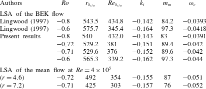
(Lingwood Reference Lingwood1997) (see table 1).
3 Results
The Reynolds number is increased step by step from zero up to
 $Re=4\times 10^{5}$
. For each increment, the steady flow solution is assumed to be reached when
 $|\boldsymbol{U}^{n+1}-\boldsymbol{U}^{n}|/\unicode[STIX]{x1D6FF}t\leqslant 10^{-5}$
, where
 $\boldsymbol{U}$
is the velocity vector, and the subscripts
 $n+1$
and
 $n$
correspond to time steps
 $(n+1)\unicode[STIX]{x1D6FF}t$
and
 $n\unicode[STIX]{x1D6FF}t$
. No extra disturbances are added. Perturbations are then measured primarily by the magnitude of the axial component of the velocity, which varies about a zero mean within the boundary layers on the disks.
3.1 Steady and mean flow
The steady flow is axisymmetric with three velocity components, due to the circulation in the meridional
 $(r,z)$
-plane, created by the centrifugal force associated with the rotation of the disk. In this meridional plane, the secondary flow is essentially radial in the two boundary layers along the disks, separated by a central core in nearly solid-body rotation, and where the azimuthal component of velocity is independent of
 $z$
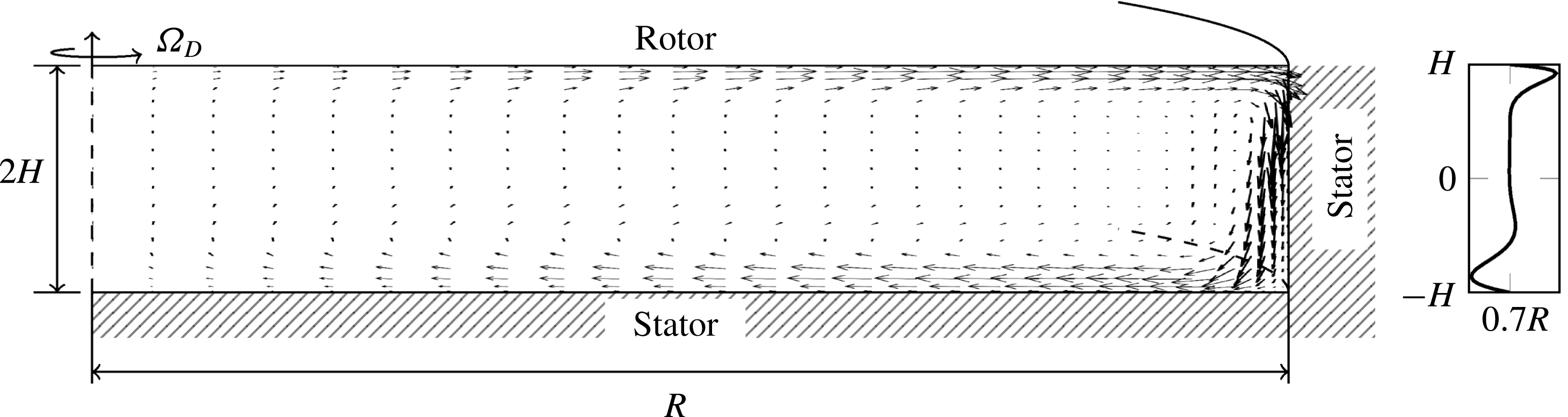
. As there is no radial flow in the central core and the cavity is closed, the radial outflow near the rotor is necessarily compensated by a radial inflow along the stator, as seen in figure 1. At high Reynolds number, the mean flow solution is obtained by averaging the solution, both in time and in the azimuthal direction.
Sketch of the rotor–stator cavity of radius
 $R$
and height
 $2H$
. Only the top disk is rotating (anti-clockwise when seen from above). Steady velocity vectors projected in the (
 $r,z$
)-plane show the secondary flow developing in the meridional plane. A typical axial profile of the mean radial velocity component is shown in the right panel, at
 $r^{\ast }=0.7R$
.

Critical values for convective absolute (c/a) transition by linear stability analysis. Present LSA results at
 $Re=4\times 10^{5}$
and comparisons with former results of Lingwood (Reference Lingwood1997) for BEK flow at various relevant Rossby numbers.
 $Ro$
and
 $r_{\unicode[STIX]{x1D6FF}}$
are the local Rossby and Reynolds numbers defined in § 2.2.
 $Re_{\unicode[STIX]{x1D6FF}}=r_{\unicode[STIX]{x1D6FF}}Ro$
is the local Reynolds number used in Lingwood (Reference Lingwood1997).
 $k_{i}$
is the spatial growth rate,
 $m_{m}$
is the most unstable azimuthal mode and
 $\unicode[STIX]{x1D714}_{c}$
is the frequency at critical conditions for the absolute instability.

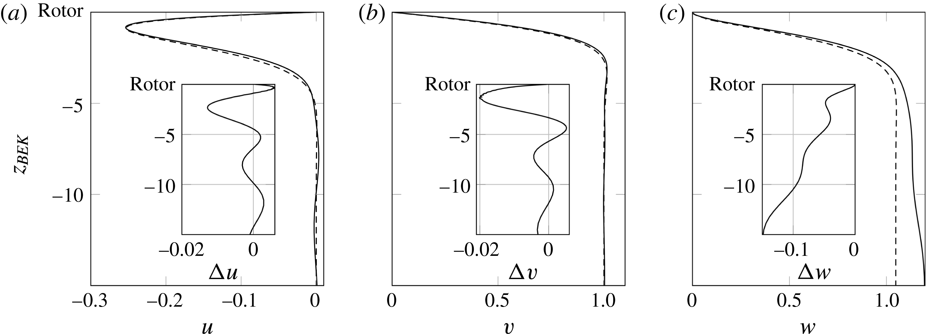
Comparisons of the velocities near the rotor between the mean flow solution —— at
 $r=7.2$
and
 $Re=4\times 10^{5}$
, and the BEK self-similarity solution – – – for
 $Ro=-0.72$
(mean
 $Ro$
of the mean flow): (a) radial velocity
 $u_{BEK}$
and
 $\bar{u}$
(b) azimuthal velocity
 $v_{BEK}$
and
 $\bar{v}$
and (c) axial velocity
 $w_{BEK}$
and
 $\bar{w}$
. The insets show the differences
 $\unicode[STIX]{x0394}\boldsymbol{u}=\boldsymbol{u}_{BEK}-\bar{\boldsymbol{u}}$
. Here, the length and velocities are scaled as in Lingwood (Reference Lingwood1997), i.e.
 $\unicode[STIX]{x1D6FF}$
,
 $r^{\ast }\unicode[STIX]{x1D6FA}^{\ast }Ro$
for
 $u$
and
 $v$
and
 $\unicode[STIX]{x1D6FA}^{\ast }Ro$
for
 $w$
, where the superscript
 $^{\ast }$
indicates dimensional values, and
 $\unicode[STIX]{x1D6FA}^{\ast }$
and
 $Ro$
are defined in (2.1).

Far from the rotor edge, the mean velocity profiles are very close to those of the von Kármán self-similarity solution (not shown). The Rossby number is nearly constant over the radius, with variations of less than
 $2\,\%$
in the range of
 $Ro\in [-0.73;-0.7]$
. Due to radial confinement, however, the differences between the BEK profiles and the mean flow grow when approaching the edge (growing
 $r_{\unicode[STIX]{x1D6FF}}$
). These differences are exemplified in figure 2 for
 $r=7.2$
at
 $Re=4\times 10^{5}$
. This departure of the velocity profiles from the BEK flow induces a decrease of
 $r_{\unicode[STIX]{x1D6FF}_{c/a}}$
for the same Rossby number, as shown in the table 1. The discrepancy in the local critical Reynolds numbers even grows as
 $r$
is increased from
 $4.6$
to
 $7.2$
. LSA of the mean flow shows how sensitive the stability properties are to variations in the velocity profiles. Indeed, the large reduction of the critical Reynolds number
 $(r_{\unicode[STIX]{x1D6FF}_{c/a}}=492\rightarrow 425)$
as
 $r$
is increased from
 $4.6$
to
 $7.2$
cannot be attributed to the small variation of the Rossby number
 $(Ro=-0.72\rightarrow -0.71)$
governing the stability of the BEK flow. It actually turns out that this shifted critical Reynolds number can be accounted for by the small changes in the
 $\bar{u}$
and
 $\bar{v}$
profiles rather than the changes in the
 $\bar{w}$
profiles. This is related to the different scalings prevailing for the radial and azimuthal components of the velocity,
 $r^{\ast }\unicode[STIX]{x1D6FA}^{\ast }Ro$
, and for the vertical component,
 $\unicode[STIX]{x1D6FA}^{\ast }Ro$
,
 $r^{\ast }$
being of the order of
 $O(10^{2})$
near the critical limit (see Lingwood Reference Lingwood1997).
3.2 Unsteady flows and solution patterns in the cavity
Typical solution patterns in the whole cavity are shown at the largest Reynolds number considered in this work
 $(Re=4\times 10^{5})$
in figure 3. The stator boundary layer (which will be not discussed further) is already turbulent and characterized by a nearly axisymmetric pattern, except in a small flow region around the axis, where the flow remains stable (see Serre et al.
Reference Serre, Tuliszka-Sznitko and Bontoux2004). This small region of stable flow damps any perturbation flowing inward along the stator, before it enters the rotor boundary layer.
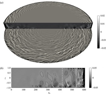
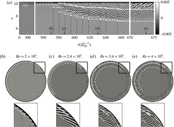
The rotor boundary layer, which is more stable than the stator one, becomes unstable at large radii. Spiral arms form a regular pattern, followed downstream by a temporally and spatially disorganized state, characteristic of incipient turbulence, as seen in figure 3(a). As already observed in an open cavity by Viaud et al. (Reference Viaud, Serre and Chomaz2011), the transition to turbulence is characterized by a shortening of the radial wavelength of the vortices, from
 $\unicode[STIX]{x1D706}\sim 25.5\unicode[STIX]{x1D6FF}$
at
 $r_{\unicode[STIX]{x1D6FF}}\sim 420$
to
 $\unicode[STIX]{x1D706}\sim 15.6\unicode[STIX]{x1D6FF}$
at
 $r_{\unicode[STIX]{x1D6FF}}>538$
, as seen in figure 3(b). This is supported by theoretical results, which predict a shift of approximately
 $30\,\%$
, from
 $\unicode[STIX]{x1D706}\sim 29\unicode[STIX]{x1D6FF}$
to
 $\unicode[STIX]{x1D706}\sim 20\unicode[STIX]{x1D6FF}$
, between the linear absolute instability analysis (Lingwood Reference Lingwood1997, only valid ahead of the front where the amplitudes of the fluctuations are small), and the saturated wave developing further downstream (Pier Reference Pier2003).
Instantaneous flow pattern in the whole cavity for
 $Re=4\times 10^{5}$
. The stator is below. Iso-surfaces and iso-contours of the instantaneous axial velocity
 $w$
. (a) Three-dimensional view. The rotor and stator boundary layers are shown for
 $z=\pm 0.97H$
, respectively. (b)
 $(r,z)$
-plane. The white dashed and solid lines in (b) show the position of the spiral pattern at
 $r_{\unicode[STIX]{x1D6FF}}\sim 420$
and the beginning of the turbulent region for
 $r_{\unicode[STIX]{x1D6FF}}>538$
, respectively (see figure 4 for a definition).

Temporal evolution of the flow patterns in the rotor boundary layer (
 $z=0.97$
) for
 $Re\in [2\times 10^{5},4\times 10^{5}]$
. Stabilization of the solution is reached before the Reynolds number is increased again. (a) Spatio-temporal diagram at
 $\unicode[STIX]{x1D703}=0$
, for
 $r\in [5,10.26]$
. The time axis is contracted for
 $t\lesssim 550$
(
 $Re<2\times 10^{5}$
), where the flow remains stable, while it is expanded for
 $t\in [670~673]$
, to magnify the unstable solution. Vertical black lines indicate instants when
 $Re$
is increased by
 $2\times 10^{4}$
. (b–e) Instantaneous top views of axial velocity field
 $w$
corresponding to four
 $Re$
, at time instants as indicated on (a). The colour bar range in (b) is exaggerated 5 times than the one of (a) otherwise the colour bar ranges for (c–d) are the same as (a). The squares below correspond to zoomed plots. The white dashed (– – –) and solid (——) lines in (a–e) show the positions of the primary
 $(1/2\log (E)>-4)$
and secondary fronts (first peak after the primary front where
 $\unicode[STIX]{x2202}E/\unicode[STIX]{x2202}r>0.02$
), respectively, with
 $E$
the kinetic energy of the perturbation defined in (3.1). The white dotted line
 $(\cdots \!)$
in (a) is
 $r=r_{\unicode[STIX]{x1D6FF}_{c/a}}G/\sqrt{Re\unicode[STIX]{x1D6FA}^{\ast }\unicode[STIX]{x1D6FA}_{D}^{-1}}$
with
 $r_{\unicode[STIX]{x1D6FF}_{c/a}}=425$
from table 1.

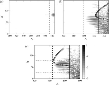
Logarithm of energy in the spectral space of the axial velocity component as a function of the local Reynolds number
 $r_{\unicode[STIX]{x1D6FF}}$
at
 $z=0.97$
: (a)
 $Re=2\times 10^{5}$
, (b)
 $Re=3\times 10^{5}$
and (c)
 $Re=4\times 10^{5}$
. The colour scales are normalized by the maximum amplitudes of the non-axisymmetric components. The arrow in (a) indicates
 $m=82$
and the solid and dashed vertical lines correspond the primary and secondary fronts, as defined in figure 4. The triangles correspond to the
 $m$
-specific c/a boundaries computed by LSA of the mean flow at the primary front locations. The horizontal lines (-
 $\cdot$
-) in (c) indicate the smallest and the largest modes,
 $m_{1}=32$
and
 $m_{2}=78$
, respectively.

The temporal evolution of
 $w$
in the rotor boundary layer is shown in figure 4, as the global Reynolds number is increased from rest. Each vertical black line in figure 4(a) (for
 $t>550$
) indicates a Reynolds number increment of
 $2\times 10^{4}$
, from
 $Re=2\times 10^{5}$
to
 $4\times 10^{5}$
. As no visible change occurs until
 $Re=2\times 10^{5}$
(
 $t\sim 550$
), the time scale has been reduced to save space. On the other hand, the time scale has been blown up on the last three time units
 $(t=670{-}673)$
to detail the unstable flow dynamics at
 $Re=4\times 10^{5}$
.
The first instability pattern occurs at the edge, at
 $Re=2\times 10^{5}$
(figure 4
b). Although parameters (
 $r_{\unicode[STIX]{x1D6FF}}$
,
 $Ro$
) are in the range of characteristic values predicted for the local, type I, absolute instability of the corresponding BEK flow, instability occurs here at a much smaller local radius,
 $r_{\unicode[STIX]{x1D6FF}}=410$
, compared to
 $r_{\unicode[STIX]{x1D6FF}_{c/a}}=530$
predicted by LSA for BEK flow. The pattern is characterized by
 $82$
spiral arms, counter-rotating with respect to the rotor at frequency
 $\unicode[STIX]{x1D714}=\unicode[STIX]{x1D714}^{\ast }\unicode[STIX]{x1D6FF}^{\ast }/(\unicode[STIX]{x1D6FA}^{\ast }r^{\ast }Ro)\simeq -0.043$
. Increasing the global Reynolds number moves these spiral arms radially inward in the rotor boundary layer, the position of the front scaling like
 $Re^{-1/2}$
. This feature is shown by the proximity of the dashed and dotted lines defined in the caption of figure 4(a). This relation is demonstrated with
 $r=r_{\unicode[STIX]{x1D6FF}_{c/a}}G/\sqrt{Re\unicode[STIX]{x1D6FA}^{\ast }\unicode[STIX]{x1D6FA}_{D}^{-1}}$
since
 $r_{\unicode[STIX]{x1D6FF}}=r^{\ast }/\unicode[STIX]{x1D6FF}=r/G\sqrt{Re\unicode[STIX]{x1D6FA}^{\ast }\unicode[STIX]{x1D6FA}_{D}^{-1}}$
.
For large Reynolds numbers
 $(Re>2.4\times 10^{5})$
, the spiral arms are followed downstream by incipient turbulence, as indicated by the white solid line in figure 4 (the definition of which is given in the caption). For the highest
 $Re$
(figure 4
e), turbulence is observed above
 $r_{\unicode[STIX]{x1D6FF}}\simeq 538$
, corresponding to a non-dimensional radius
 $r\sim 9$
. Although still coherent, spiral arms at this Reynolds number exhibit some ripples suggesting interactions between azimuthal modes. This point is supported by the spectrum in the azimuthal wavenumber
 $m$
at each
 $r_{\unicode[STIX]{x1D6FF}}$
shown in figure 5 for the flows at three different global Reynolds numbers
 $Re$
. Several azimuthal wavenumbers
 $m$
become unstable at large radii, in a range
 $m\in [75,91]$
at
 $Re=2\times 10^{5}$
,
 $m\in [39,75]$
at
 $Re=3\times 10^{5}$
to
 $m\in [32,78]$
at
 $Re=4\times 10^{5}$
, the most energetic wavenumbers being
 $m=82,64$
and
 $66$
, respectively. Horizontal lines in figure 5(c) delimit the group of the most energetic azimuthal wavenumbers in the range
 $m\in [32,78]$
, these bounds being the lowest and largest wavenumbers satisfying
 $0.5\log (\int _{0}^{r_{edge}}{\mathcal{E}}_{w}(r,m)\text{d}r)>-1.8$
, where
 ${\mathcal{E}}_{w}(r,m)$
is the Fourier energy of the axial velocity.
For each azimuthal wavenumber
 $m$
, a specific LSA is conducted, based on the mean flow at the location of the primary front
 $r_{\unicode[STIX]{x1D6FF}_{front}}$
, where the spiral starts to develop (defined in the caption of figure 4). The variability of the flow is weak at this location, and the mean flow is assumed to depart weakly from the base flow. The
 $m$
-specific c/a boundaries obtained by LSA are indicated by triangles. Compared to the spectral density plots, it appears that azimuthal modes grow upstream of the local c/a transitions. Although
 $m=82$
spiral arms are observed in DNS for
 $Re=2\times 10^{5}$
, the LSA of the mean flow leads to a convective instability. At
 $Re=3\times 10^{5}$
(figure 5
b), azimuthal wavenumbers grow and saturate close to
 $r_{\unicode[STIX]{x1D6FF}_{front}}=420$
, whereas, according to LSA, the first mode becomes absolutely unstable at
 $r_{\unicode[STIX]{x1D6FF}_{c/a}}=450$
. The flow is strongly convective at the front. This flow behaviour is similar to recent experimental measurements on a single disk where surface roughness is accounted for (Imayama et al.
Reference Imayama, Alfredsson and Lingwood2016). However, when the global Reynolds number is increased (
 $Re=4\times 10^{5}$
, figure 5
c), the c/a boundary obtained by LSA of the mean flow matches the front location obtained by DNS, meaning that the mean flow is marginally absolute at the front. This feature is similar to what is observed in experiments with clean disks or in former DNS performed either on single disk (Appelquist et al.
Reference Appelquist, Schlatter, Alfredsson and Lingwood2016) or in an azimuthal sector of an open cavity (Viaud et al.
Reference Viaud, Serre and Chomaz2011).
3.3 Steep-fronted global modes
These patterns of instability are now investigated in the framework of the front-forming, elephant, global modes. The turbulent kinetic energy
 $E$
, corresponding to the total kinetic energy of the velocity perturbation
 $(u^{\prime },v^{\prime },w^{\prime })$
, is defined within the rotor boundary layer at
 $z=0.97$
as
 $$\begin{eqnarray}\left.E(r)=\frac{r}{2}\int _{0}^{2\unicode[STIX]{x03C0}}({u^{\prime }}^{2}+{v^{\prime }}^{2}+{w^{\prime }}^{2})\,\text{d}\unicode[STIX]{x1D703}\right|_{rotor}.\end{eqnarray}$$
Using Parseval’s identity, this energy can be split over the contribution of each azimuthal wavenumber
 $m$
, denoted
 $E_{m}$
. Radial variations of
 $\log (E)$
for various global Reynolds numbers are plotted in figure 6 as a function of both the physical radius
 $r$
and the local Reynolds parameter
 $r_{\unicode[STIX]{x1D6FF}}$
, for
 $0\leqslant r_{\unicode[STIX]{x1D6FF}}\leqslant 600$
. Note that the maximum of
 $r_{\unicode[STIX]{x1D6FF}}$
,
 $r_{\unicode[STIX]{x1D6FF}_{edge}}$
, varies with
 $Re$
since
 $r_{\unicode[STIX]{x1D6FF}_{edge}}\propto r\sqrt{Re\unicode[STIX]{x1D6FA}^{\ast }}$
. At large global Reynolds numbers, the rotation rate
 $\unicode[STIX]{x1D6FA}^{\ast }\simeq 0.91$
, and remains almost constant in space, except near the edge. At each
 $Re$
, the value of the perturbation is taken at the last computing time, when the flow is steady.
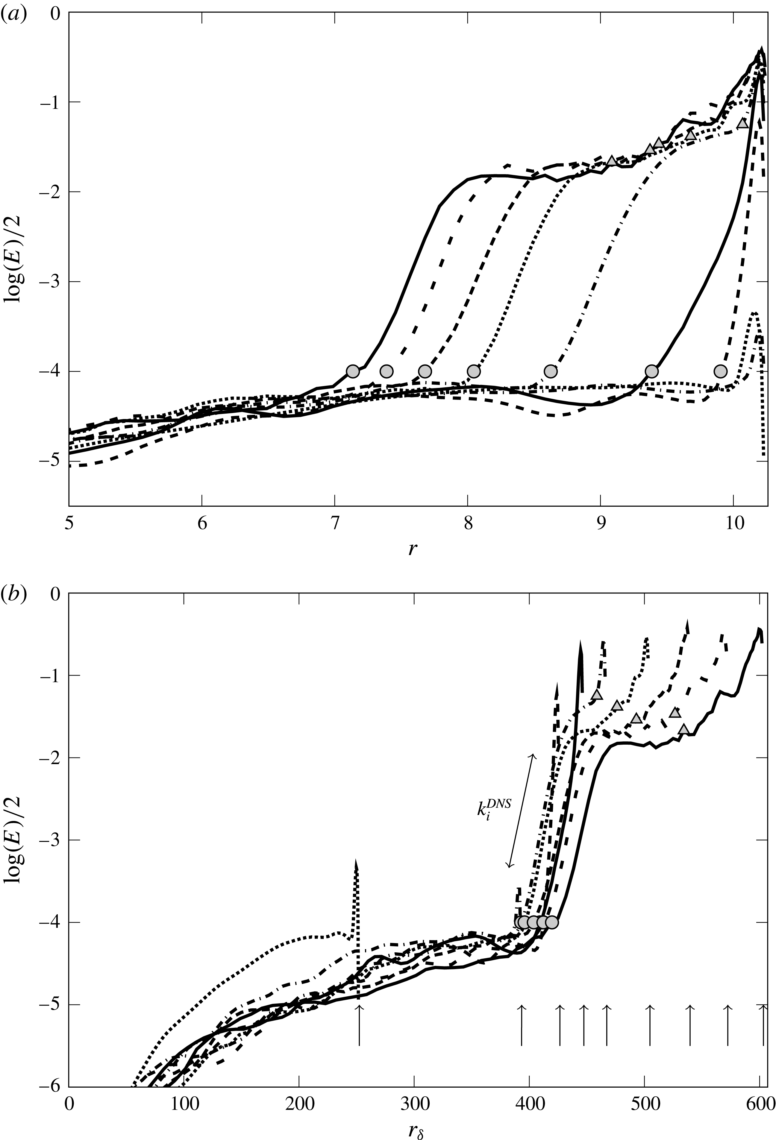
Radial profiles of the turbulent kinetic energy
 $E$
in the rotor boundary layer at
 $z=0.97$
, and for various global Reynolds numbers:
 $\cdots \,$
 $Re=0.7\times 10^{5}$
; -
 $\cdot$
-
 $Re=1.7\times 10^{5}$
; - - -
 $Re=2\times 10^{5}$
; —
 $Re=2.2\times 10^{5}$
; -
 $\cdot$
-
 $Re=2.4\times 10^{5}$
;
 $\cdots \,$
 $Re=2.8\times 10^{5}$
; - -
 $Re=3.2\times 10^{5}$
; - - -
 $Re=3.6\times 10^{5}$
and —
 $Re=4\times 10^{5}$
. The symbols represent the locations of the primary (○) and the secondary fronts (▵) as defined in figure 4. The arrows in (b) indicate the edge local Reynolds number
 $r_{\unicode[STIX]{x1D6FF}_{edge}}$
(maximum value of
 $r_{\unicode[STIX]{x1D6FF}}$
) for each
 $Re$
.

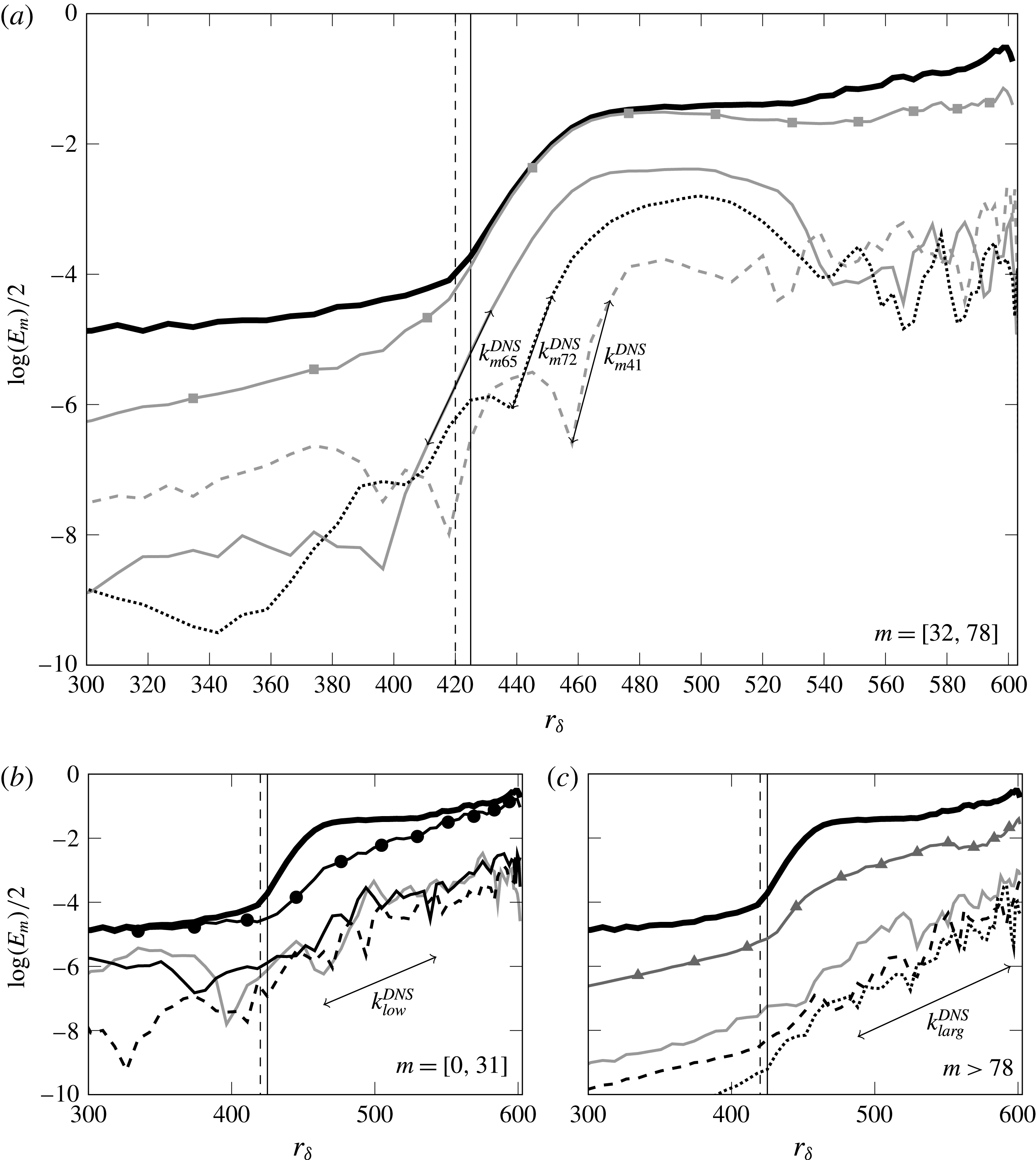
Kinetic energies of the perturbation for some selected azimuthal wavenumbers
 $m$
in the ranges of (a) intermediate
 $m\in [32,78]$
:
 $m=41$
– – –,
 $m=65$
—— and
 $m=72$
 $\cdots \,$
(b) low
 $m=[0,32]$
:
 $m=0$
——,
 $m=10$
—— and
 $m=30$
– – –, (c) large
 $m>78$
:
 $m=90$
——,
 $m=118$
– – – and
 $m=140$
 $\cdots \,$
at
 $Re=4\times 10^{5}$
. The thick black lines show the total energy (
 $1/2\log (E)$
) shown in figure 6 and lines with symbols show the total energy restricted to each range. The vertical solid line indicates the absolute instability transition
 $r_{\unicode[STIX]{x1D6FF}_{c/a}}=425$
of the mean flow and dashed line represents the primary front of DNS defined in figure 4. The spatial growth rates are estimated as
 $k_{i,m41}^{DNS}=-0.18$
,
 $k_{i,m65}^{DNS}=-0.1$
,
 $k_{i,m72}^{DNS}=-0.13$
and for low and large
 $m$
, the spatial growth rates are approximately estimated as
 $k_{i,low}^{DNS}\simeq -0.014$
and
 $k_{i,larg}^{DNS}\simeq -0.019$
.

For
 $r_{\unicode[STIX]{x1D6FF}_{edge}}\lesssim 393~(Re<1.7\times 10^{5})$
, the boundary layer remains undisturbed over most of the rotor surface, and the
 $E$
-profiles only show small-amplitude peaks in the vicinity of the edge (approximately 4 times larger than the background noise). This indicates that the flow close to the rotor edge is unstable, and may act as a source of perturbations. At
 $r_{\unicode[STIX]{x1D6FF}_{edge}}\simeq 427$
(see the curve plotted in figure 6 for
 $Re=2\times 10^{5}$
), the peak at the edge is still visible, but with a kinetic energy increased by about two orders of magnitude. This is related to the sharply peaked
 $m=82$
azimuthal mode observed in figure 5(a), and characterized by spiral arms forming a regular front located in a very narrow region near the edge, as seen in figure 4(a). Its spatial growth rate, estimated from the corresponding energy profile in figure 6, is
 $k_{i}^{DNS}=-0.2$
.
For larger Reynolds numbers,
 $r_{\unicode[STIX]{x1D6FF}_{edge}}\gtrsim 447~(Re\geqslant 2.2\times 10^{5})$
, the front moves inward (in term of physical radius
 $r$
), as shown in figure 6(a). Whatever the Reynolds number, fluctuations start growing around
 $r_{\unicode[STIX]{x1D6FF}}\simeq 400$
(black circular symbols in figure 6
b) and saturate around
 $r_{\unicode[STIX]{x1D6FF}}\simeq 450$
, with an energy approximately two orders of magnitude larger. Thus, the front location predicted by DNS does not substantially change with
 $r_{\unicode[STIX]{x1D6FF}_{edge}}$
(figure 6
b). The front may appear upstream of the local c/a boundary predicted by LSA, but this theoretical location gets progressively closer to the front when increasing the Reynolds number. At
 $Re=4\times 10^{5}$
, the front location matches well with the critical Reynolds number for the local absolute instability predicted by LSA (
 $r_{\unicode[STIX]{x1D6FF}_{front}}\simeq 420$
compared to
 $r_{\unicode[STIX]{x1D6FF}_{c/a}}=425$
in table 1). The mean
 $\bar{w}$
-profile at a radial location changes when increasing the Reynolds number, thus leading to more unstable local stability properties.
Compared to smaller Reynolds number cases (
 $Re\leqslant 2\times 10^{5}$
), the spatial growth rates of these fronts are smaller, and keep the same value
 $k_{i}^{DNS}\simeq -0.07$
, whatever the
 $r_{\unicode[STIX]{x1D6FF}_{edge}}$
. This value is about two times smaller than the spatial growth rate of local absolute instability (
 $k_{i}$
predicted by LSA (table 1)) as well as the growth rate usually measured in the literature when computations are restricted to an azimuthal sector (Viaud et al.
Reference Viaud, Serre and Chomaz2011; Appelquist et al.
Reference Appelquist, Schlatter, Alfredsson and Lingwood2016). However, it matches very well the experimental measurements carried out on a single disk by Imayama et al. (Reference Imayama, Alfredsson and Lingwood2013),
 $k_{i}^{EXP}\simeq -0.065$
, and reported in figure 4 of their paper. Although the Rossby numbers
 $Ro$
in this study and the other studies differ, the spatial growth rate does not vary substantially from
 $Ro=-1$
to
 $Ro=-0.7$
. To clarify this point, the flow dynamics has been decomposed into three sets of azimuthal wavenumbers, according to its energy level as computed in figure 5(c): the most energetic modes
 $m_{1}\leqslant m\leqslant m_{2}$
and two other sets with lower energy, the low azimuthal wavenumber modes
 $m\leqslant m_{1}-1$
, and the high azimuthal wavenumber modes such
 $m\geqslant m_{2}+1$
. The azimuthal wavenumbers
 $m_{1}$
and
 $m_{2}$
are shown in figure 5(c). Figure 7 shows the kinetic energies
 $E_{m}$
for some selected wavenumbers of the perturbation, chosen within the three sets, as well as the sums over the azimuthal wavenumber ranges for each set, compared to the total perturbation energy calculated on the whole spectrum. Results show that the low azimuthal wavenumber modes mostly provide energy at small and large radii, corresponding to
 $r_{\unicode[STIX]{x1D6FF}}<400$
and
 $r_{\unicode[STIX]{x1D6FF}}>550$
, respectively (figure 7
a). The most energetic modes clearly determine the slope of the steep front shown in figure 6. Interestingly, the slope of each front corresponds to a larger spatial growth rate (
 $k_{i}^{DNS}\sim -0.12$
), which is close to the value predicted by LSA for the local absolute instability of the mean flow (
 $k_{i}\sim -0.157$
, see table 1). Although each azimuthal wavenumber exhibits a steep front, their summation presents a smoother growth since the energy of each mode starts growing at various radial locations. It is gratifying that this weaker spatial growth rate is in agreement with experiments. For the highest azimuthal wavenumbers
 $m$
, the energies are low, but they still grow continuously with
 $r_{\unicode[STIX]{x1D6FF}}$
, as depicted in figure 7(c).
4 Summary and concluding remarks
The laminar–turbulent transition of the incompressible rotating disk boundary layer has been investigated by DNS and LSA of the mean flow in a closed cylindrical rotor–stator cavity. In the DNS, the global Reynolds number
 $Re$
is increased incrementally from zero, and no artificial perturbation is superimposed to the flow. Unlike all former DNS studies in the literature, both in single disk and in cavity configurations, the simulations are not restricted to an azimuthal sector of the cavity and thus include all nonlinear interactions. The main findings of this study can be summarized as follows:
(i) Over a large radial extent, the steady boundary layers developing over the rotor of the cavity match the von Kármán self-similarity solutions calculated at corresponding Rossby numbers. The mean velocity profiles in the cavity, nevertheless, increasingly depart from the von Kármán solution as the edge is approached. These differences explain why the LSA yields a more unstable configuration in the case of the mean flow in the cavity than in the case of the self-similarity solution. Moreover, at the rotor edge, the flow is a radial wall jet impacting the shroud combined with a centrifugally unstable vertical boundary layer. That leads to a very unstable flow at the edge, associated with strong fluctuations observed at all investigated Reynolds numbers.
(ii) At moderate Reynolds numbers, corresponding to
 $r_{\unicode[STIX]{x1D6FF}_{edge}}\lesssim 426$
, strong fluctuations are observed at the edge. These fluctuations are associated with the occurrence of a steep front (corresponding spatial growth rate
$k_{i}^{DNS}\simeq -0.2$
), and are followed downstream by a spiral pattern presenting
$m=82$
arms. This pattern is observed at a local Reynolds number
$r_{\unicode[STIX]{x1D6FF}}$
smaller than the value
$r_{\unicode[STIX]{x1D6FF}_{c/a}}$
predicted by LSA for the local convective absolute transition. This discrepancy suggests that the corresponding global mode is driven by the edge, with a scaling constant in
$r$
and varying with
$r_{\unicode[STIX]{x1D6FF}edge}$
. It can be somewhat surprising that, although the mode properties are in favour of an edge-driven mode, the dominant wavenumber
$m=82$
is consistent with the edge-independent theory of Lingwood (Reference Lingwood1997).
(iii) At large Reynolds numbers
$(r_{\unicode[STIX]{x1D6FF}_{edge}}\gtrsim 447)$
, fluctuations still take the form of a steep front followed by a saturated spiral wave. The characteristics of theses fronts are now independent of the Reynolds number at the edge (
$r_{\unicode[STIX]{x1D6FF}_{edge}}$
), and this may be accounted for by a self-sustained rotor boundary layer global mode. The spatial growth along the radial direction of the energy of these fluctuations is quantitatively similar to that observed experimentally by Imayama et al. (Reference Imayama, Alfredsson and Lingwood2014), and corresponds to a spatial growth rate two times smaller than theoretically predicted for local absolute instability threshold
$(k_{i}^{DNS}\simeq -0.07,k_{i}^{EXP}\simeq -0.065,k_{i}\simeq -0.157)$
. Table 2 summarizes present results, compared to existing experimental and numerical results in Imayama et al. (Reference Imayama, Alfredsson and Lingwood2014) and Appelquist et al. (Reference Appelquist, Schlatter, Alfredsson and Lingwood2016). Although the Rossby numbers differ, the present DNS over a full disk quantitatively retrieve the experimental spatial growth rate. Comparing the full disk DNS to LSA in our rotor–stator set-up also qualitatively explains by the coexisting azimuthal wavenumbers the differences previously observed between sector DNS (and LSA) and experiments. A similar argument could also apply to explain the differences previously observed in the temporal frequencies.(iv) The azimuthal spectral analysis of the solutions at these Reynolds numbers shows that the spiral front results from the superposition of several absolutely unstable modes associated with azimuthal wavenumbers in the range
$m\in [32,78]$
. Interestingly, the spatial growth rates for each
$m$
match the theoretical value of the LSA for
$m=76$
(given table 1). The slopes measured in figure 5(b) are indeed almost similar for all
$m$
in the range
$m\in [32,78]$
, with
$k_{i}^{DNS}=[-0.18,-0.1]$
, compared to the results of the LSA in range
$k_{i}^{LSA}\sim [-0.2,-0.157]$
.(v) At the large rotation rates presently studied, a secondary front is also conspicuously close to
$r_{\unicode[STIX]{x1D6FF}}^{DNS}=538$
and immediately followed by incipient turbulence.








Summary of present results in comparison to the experimental and DNS data for
 $Ro=-1$
. Here,
 $r_{\unicode[STIX]{x1D6FF}c}$
varies depending on the definition of the characteristic location: for (Imayama et al.
Reference Imayama, Alfredsson and Lingwood2014; Appelquist et al.
Reference Appelquist, Schlatter, Alfredsson and Lingwood2016)
 $r_{\unicode[STIX]{x1D6FF}_{end}}$
where the linear region ends and for
 $r_{\unicode[STIX]{x1D6FF}_{front}}$
for the present DNS. The spatial growth rate
 $k_{i}$
is estimated near the
 $r_{\unicode[STIX]{x1D6FF}c}$
. The frequency
 $\unicode[STIX]{x1D714}$
is defined as
 $\unicode[STIX]{x1D714}=\unicode[STIX]{x1D714}^{\ast }/\unicode[STIX]{x1D6FA}_{D}$
and the theoretical value
 $\unicode[STIX]{x1D714}_{c}^{\ast }$
is the converted vale of
 $\unicode[STIX]{x1D714}_{c}$
to the same scaling as
 $\unicode[STIX]{x1D714}_{c}^{\ast }=\unicode[STIX]{x1D714}_{c}Re_{\unicode[STIX]{x1D6FF}_{c/a}}-m_{m}$
.

The present results bring new insights to the way that turbulence occurs in the rotating disk boundary layer. In agreement with recent experimental observations of Pier (Reference Pier2013) in a single disk configuration, two distinct mechanisms can be identified for the onset of turbulence. At small Reynolds numbers, before the flow transition from convective to absolute instability, fluctuations start rising at the edge, within a region where the flow is no longer similar to the von Kármán boundary layer, and where shear and centrifugal effects cause a strong instability. This region acts as a strong source of perturbations. This mechanism is related to finite-size effects of the cavity, and leads to a global mode which is obviously driven by the edge. At large Reynolds numbers, fluctuations take the form of a front the radial location of which is nearly fixed in
 $r_{\unicode[STIX]{x1D6FF}}$
, independently of the flow conditions at the edge. This can be interpreted as a self-sustained global mode developing in the rotor boundary layer and exhibiting a steeper front. Such a behaviour had been previously observed in DNS in azimuthal sectors (Viaud et al.
Reference Viaud, Serre and Chomaz2008, Reference Viaud, Serre and Chomaz2011; Appelquist et al.
Reference Appelquist, Schlatter, Alfredsson and Lingwood2016). But unlike previous DNS, the spatial growth rate of the front in the present DNS, which is approximately twice smaller than predicted by LSA, matches also well with experimental measurements of Imayama et al. (Reference Imayama, Alfredsson and Lingwood2013). It is the superposition of various absolutely unstable modes with different azimuthal wavenumbers that accounts for this gentler front. These results can be viewed as a collection of elephant global modes whose the superposition would lead to a smoother integrated energy variation in
 $r$
.
This result explains the discrepancy observed in the growth rate values between LSA and DNS in azimuthal sectors on the one side, and experiments and the present simulations on the other side. It also shows that fully nonlinear simulations are required to reproduce experimental observations. It would seem, thus, that convective modes produced by steady roughness are not necessary to explain this disagreement. The fact that, in the present DNS, the
 $m$
-dependent front associated with each individual azimuthal wavenumber develops upstream of the
 $m$
-specific convective absolute boundary remains unexplained at this point. This could be related to the fact that the LSA is performed on the numerical mean flow instead of the steady base flow, or to a weak forcing through the inertial wave, and we are currently working along those lines.
To finally address the transition to turbulence, the scenario seems to involve a secondary instability, characterized by a second front occurring downstream of the first one. At
 $Re=4\times 10^{5}$
, the highest Reynolds number of the present study, the secondary front rises in the lee of the first and it is immediately followed by incipient turbulence. This flow behaviour is similar to that observed in DNS of azimuthal sectors of a rotating open cavity (Viaud et al.
Reference Viaud, Serre and Chomaz2011), or of a single disk (Appelquist et al.
Reference Appelquist, Schlatter, Alfredsson and Lingwood2016). Further investigations at higher Reynolds numbers are however required to better characterize this secondary instability and its role in the transition scenario.
Acknowledgements
This work was supported by the Labex MEC (ANR-10-LABX-0092) funded by the Investissements d’Avenir program of the French National Research Agency (ANR). This work was granted access to the HPC resources of Aix-Marseille University under the project Equip@Meso (ANR-10-EQPX-29-01) and of IDRIS, under the allocation i20170242 made by GENCI.