1 Introduction
Lagrangian particle trajectories in steady flows are strongly influenced by the presence of hyperbolic (saddle-like) stagnation points, and their attached stable (respectively, unstable) manifolds consisting of particles that approach each stagnation point asymptotically in forward (respectively, backward) time (Guckenheimer & Holmes Reference Guckenheimer and Holmes1983; Wiggins Reference Wiggins1992). The same is true in idealized unsteady flows, but in this case the hyperbolic stagnation points generalize to hyperbolic trajectories, to which are also attached stable and unstable manifolds, although now all these entities move with time. Stable (respectively, unstable) manifolds are flow separators in forward (respectively, backward) time, demarcating, for example, boundaries between different coherent structures in flows (Rom-Kedar, Leonard & Wiggins Reference Rom-Kedar, Leonard and Wiggins1990; Pierrehumbert Reference Pierrehumbert1991; Samelson Reference Samelson1992; Peacock & Haller Reference Peacock and Haller2013). Therefore, transport can be enhanced by breaking these barriers in various ways (Rom-Kedar et al. Reference Rom-Kedar, Leonard and Wiggins1990; Wiggins Reference Wiggins1992; Stroock et al. Reference Stroock, Dertinger, Adjari, Mezić, Stone and Whitesides2002; Grigoriev Reference Grigoriev2005; Balasuriya Reference Balasuriya2010, Reference Balasuriya2015a ; Mezić et al. Reference Mezić, Loire, Fonoberov and Hogan2010; Balasuriya & Finn Reference Balasuriya and Finn2012; Balasuriya Reference Balasuriya2015b ).
Because of its deep connections to mixing and transport, there has been significant effort devoted to developing metrics for locating and characterizing hyperbolicity in fluid flows. Ideally, one desires finite regions with hyperbolic character, as these regions can be considered to be the most strongly mixing parts of the flow. Early work focused on the intuitive (although somewhat fraught (Haller Reference Haller2005)) similarity between hyperbolicity and strain, and ellipticity and rotation, and used the local velocity gradient as an indicator for hyperbolic or elliptic structures. This approach led to, for example, the so-called
 $Q$
-criterion, (Hunt, Wray & Moin Reference Hunt, Wray and Moin1988), the
 $\unicode[STIX]{x1D6E5}$
-criterion (Chong, Perry & Cantwell Reference Chong, Perry and Cantwell1990) and the
 $\unicode[STIX]{x1D706}_{2}$
-criterion (Jeong & Hussain Reference Jeong and Hussain1995), all of which consider (in slightly different forms) the local balance between strain and rotation. In two-dimensional flows, the analogous quantity is often known as the Okubo–Weiss criterion (Okubo Reference Okubo1970; Weiss Reference Weiss1991); and we note that higher-order corrections to the Okubo–Weiss criterion that involve the acceleration in the flow have also been developed (Basdevant & Philipovitch Reference Basdevant and Philipovitch1994; Hua & Klein Reference Hua and Klein1998). All of these measures, however, have flaws as indicators of true hyperbolic and elliptic regions in unsteady flows (Haller Reference Haller2005). These methods will all, for example, misidentify a pure straining field in a rotating frame of reference as a pure vortex.
Doing a better job of locating real hyperbolic and elliptic structures in relation to their transport implications for nearby fluid particles necessitates a Lagrangian framework, which casts the evolution of the flow into a form more explicitly compatible with dynamical systems theory. More importantly, Lagrangian analysis incorporates the unsteadiness of the flow field in an intrinsic and natural way, so that the structures found are guaranteed to be relevant for the evolution of the flow. A range of methods have been, and continue to be, developed to locate Lagrangian structures, including topological analyses based on braids (Allshouse & Thiffeault Reference Allshouse and Thiffeault2012; Budišić & Thiffeault Reference Budišić and Thiffeault2015), sets whose boundaries retain their curvature (Ma & Bollt Reference Ma and Bollt2014), ergodic partitions and entropy (Budišić & Mezić Reference Budišić and Mezić2012; Froyland & Padberg-Gehle Reference Froyland and Padberg-Gehle2012), clustering (Froyland & Padberg-Gehle Reference Froyland and Padberg-Gehle2015; Huntley et al. Reference Huntley, Lipphardt, Jacobs and Kirwan2015), Perron–Frobenius transfer operator methods that help determine regions that ‘hold together’ (Froyland & Padberg Reference Froyland and Padberg2009; Dellnitz & Junge Reference Dellnitz and Junge2002; Froyland, Lloyd & Santitissadeekorn Reference Froyland, Lloyd and Santitissadeekorn2010), analysis of its adjoint, the Koopman operator (Mezić Reference Mezić2013) and a Lagrangian generalization of the Okubo–Weiss criterion via so-called mesochronic analysis (Mezić et al. Reference Mezić, Loire, Fonoberov and Hogan2010).
The most commonly used method for determining the most straining regions in a Lagrangian sense, however, is the finite-time Lyapunov exponent (FTLE) and related techniques (Shadden, Lekien & Marsden Reference Shadden, Lekien and Marsden2005; Lee et al. Reference Lee, Shih, Tabeling and Ho2007; Waugh, Abraham & Bowen Reference Waugh, Abraham and Bowen2007; Samelson Reference Samelson2013; Allshouse & Peacock Reference Allshouse and Peacock2015; Balasuriya Reference Balasuriya2015a ; Huntley et al. Reference Huntley, Lipphardt, Jacobs and Kirwan2015; Johnson & Meneveau Reference Johnson and Meneveau2015; He et al. Reference He, Pan, Feng, Gao and Wang2016). Over a given time period, this method computes the stretching experienced by a fluid element placed at each location, and by plotting this stretching field, one can identify maximum regions. Typically, these maxima occur along ridges, which are then extracted and interpreted as the boundaries between coherent structures. The maximum stretching property is consonant with the similar property exhibited by stable and unstable manifolds (Guckenheimer & Holmes Reference Guckenheimer and Holmes1983) in infinite-time flows. For steady flows, these objects are regions in space that are attracted to, or repelled from, hyperbolic (saddle-like) stagnation points. In unsteady flows, they are time-varying regions that are attracted to, or repelled from, hyperbolic trajectories that move with time (Balasuriya Reference Balasuriya2012; Balasuriya & Padberg-Gehle Reference Balasuriya and Padberg-Gehle2014). Rather than FTLEs, Haller (Reference Haller2011, Reference Haller2015) chooses to use a different property of stable and unstable manifolds in identifying what have become known as hyperbolic Lagrangian coherent structures (LCSs): namely that they are co-dimension-one entities to which there is maximal attraction or repulsion over a finite-time period of the flow. These structures are curves in two dimensions, or surfaces in three dimensions (Blazevski & Haller Reference Blazevski and Haller2014). It should be noted that the term LCS is often (and confusingly) used in the literature to refer to all of the above characterizations, although it is known that they do not in general coincide (Haller Reference Haller2015; Karrasch Reference Karrasch2015).
In this article, we seek to locate and track regions in space in which exponential stretching of fluid elements occurs. However, a fundamental difficulty in analysing finite-time unsteady flows (i.e. in any realistic data set obtained from observations or experiments) is that the growth of any smooth function can be bounded by a growth of the form
 $Ae^{\unicode[STIX]{x1D706}t}$
, where
 $\unicode[STIX]{x1D706}$
is a rate constant: for any given
 $\unicode[STIX]{x1D706}$
, one can simply choose
 $A$
large enough. This property means that the stretching rate,
 $\unicode[STIX]{x1D706}$
, is ambiguous for finite-time flows. Methods for defining hyperbolic trajectories (in infinite time) usually rely on such exponential decay estimates (Coppel Reference Coppel1978; Balasuriya Reference Balasuriya2012), which are related to the stretching of nearby fluid elements; but how can this notion be extended to finite-time situations? There are continuing attempts to resolve this issue in the time domain, for example by setting
 $A=1$
(Doan et al.
Reference Doan, Karrasch, Nguyen and Siegmund2012; Karrasch Reference Karrasch2013); but such ad hoc choices are unsatisfying. Moreover, there can be situations in which there is (intuitively) exponential stretching over some times and no stretching whatsoever over others. In other words, there are time intervals that might be associated with a particular form of exponential stretching. Revealing, or defining, this behaviour in the time domain is therefore fraught with difficulties. We offer an alternative viewpoint.
Regardless of the precise definition we take, much of our intuition about the function these structures play in the flow dynamics comes from the analogy with stable and unstable manifolds (Haller Reference Haller2015; Balasuriya Reference Balasuriya2016b ). A long-term hope is that fluid transport optimization and control based on stable and unstable manifolds (Balasuriya & Finn Reference Balasuriya and Finn2012; Balasuriya & Padberg-Gehle Reference Balasuriya and Padberg-Gehle2014) might be adaptable to finite-time flows (Ouellette, Hogg & Liao Reference Ouellette, Hogg and Liao2016). But, although inspired by properties associated with stable and unstable manifolds, hyperbolic structures in finite-time unsteady flows possess quite different characteristics. In the first place, hyperbolic structures, however they are defined, may be ephemeral. Moreover, during their existence, they will drive exponential stretching only for fluid elements that are sufficiently close. In contrast to infinite-time flows, fluid elements near a repelling LCS or a forward-time FTLE ridge (the analogues of a stable manifold in each of the characterizations) in finite-time flows may not come close enough to the associated hyperbolic trajectory to feel its effects before the hyperbolic trajectory disappears. Therefore, what we are really interested in is the region of influence, as a function of time, of each hyperbolic trajectory during its lifetime.
Here, we introduce a new way of thinking about this zone of influence, arising directly from the methods of nonlinear dynamics. Hyperbolic points or trajectories are so called because the linearized flow around them produces trajectories that are locally hyperbolæ. We therefore define the hyperbolic neighbourhood around one of these locations to be the region where the linearized flow is a good approximation to the full flow. By construction, the fluid elements in this neighbourhood feel the influence of the nearby hyperbolic structure so strongly that they will experience immediate exponential stretching, with minimal effects from the rest of the flow field. Once elements leave this region, they will no longer be so strongly influenced. Thus, elements traversing the flow domain will experience ‘exponential boosts’ to their stretching as they pass through hyperbolic neighbourhoods. The irregular spatial distribution of hyperbolic neighbourhoods, their time evolution and their appearance and disappearance therefore provide a template for the evolution of stretching in the flow field.
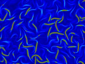
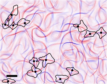
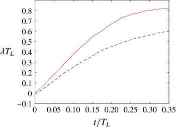
Below, in § 2, we motivate and give a precise definition of these hyperbolic neighbourhoods, and explain the role they play in organizing the stretching of fluid elements. Connections to FTLE and LCS methods are also discussed, since these techniques are of great current interest in fluid dynamics ranging from micro- to geophysical scales (Samelson Reference Samelson2013; Balasuriya Reference Balasuriya2015a ; Huntley et al. Reference Huntley, Lipphardt, Jacobs and Kirwan2015; Johnson & Meneveau Reference Johnson and Meneveau2015; Haller et al. Reference Haller, Hadjighasem, Farazmand and Huhn2016; He et al. Reference He, Pan, Feng, Gao and Wang2016; Ouellette et al. Reference Ouellette, Hogg and Liao2016). In § 3, we explicitly calculate the hyperbolic neighbourhoods for several analytical examples, including the Duffing equation, the steady Taylor–Green flow and the oscillating Taylor–Green flow. We demonstrate that residence time within hyperbolic neighbourhoods is closely connected to the FTLE fields, and that fluid elements entering these neighbourhoods markedly increase their stretching, and reduce it once they leave. We offer insights as to how the geometry of these neighbourhoods impacts interpretations that one might reach by examining FTLE fields, and indeed show that the degeneracy of the neighbourhoods can be held accountable for some instances in which FTLE fields are known to provide unexpected results. Then, to show that these neighbourhoods are indeed computable from real data, we present measurements from a turbulent quasi-two-dimensional laboratory flow in § 4. Finally, in § 5, we summarize our results, discuss the current limits of our analysis and outline what we see as the most promising paths forward.
2 Defining hyperbolic neighbourhoods
2.1 Steady flows: exponential boosts in stretching
In developing our methodology for unsteady flows, it helps to first build intuition for a steady flow given by
 $$\begin{eqnarray}\displaystyle {\dot{x}}_{i}=u_{i}(\boldsymbol{x}), & & \displaystyle\end{eqnarray}$$
where the dot denotes differentiation along a Lagrangian trajectory. Stagnation points
 $\bar{\boldsymbol{x}}$
satisfy
 $u_{i}(\bar{\boldsymbol{x}})=0$
. If
 $(\unicode[STIX]{x2202}/\unicode[STIX]{x2202}x_{j})u_{i}(\bar{\boldsymbol{x}}(t))$
has eigenvalues that are not imaginary, and with at least one with a positive real part and another with a negative real part, then
 $\bar{\boldsymbol{x}}$
is a hyperbolic point (Guckenheimer & Holmes Reference Guckenheimer and Holmes1983; Ouellette & Gollub Reference Ouellette and Gollub2008). It has attached to it stable and unstable manifolds with dimensions given by the number of real part negative and positive eigenvalues, respectively (Guckenheimer & Holmes Reference Guckenheimer and Holmes1983; Balasuriya Reference Balasuriya2012). These emanate in the directions spanned by the corresponding eigenvectors (Guckenheimer & Holmes Reference Guckenheimer and Holmes1983), and their global structure organizes the dynamics of the flow (Perry & Chong Reference Perry and Chong1987; Rom-Kedar et al.
Reference Rom-Kedar, Leonard and Wiggins1990). The eigenvalues and vectors give us this information because if the flow is linearized about the point
 $\bar{\boldsymbol{x}}$
by setting
 $\boldsymbol{x}(t)=\bar{\boldsymbol{x}}+\boldsymbol{y}(t)$
, then Taylor expansions give
 $$\begin{eqnarray}\displaystyle {\dot{y}}_{i}=y_{j}\frac{\unicode[STIX]{x2202}}{\unicode[STIX]{x2202}x_{j}}u_{i}(\bar{\boldsymbol{x}})+O(|\boldsymbol{y}|^{2}), & & \displaystyle\end{eqnarray}$$
and neglecting higher-order term tells us that the velocity is locally linear in
 $\boldsymbol{y}$
. If
 $\boldsymbol{y}(0)$
were chosen in an eigenvector direction corresponding to an eigenvalue
 $\unicode[STIX]{x1D706}$
of
 $(\unicode[STIX]{x2202}/\unicode[STIX]{x2202}x_{j})u_{i}(\bar{\boldsymbol{x}})$
(i.e.
 $\unicode[STIX]{x1D735}\boldsymbol{u}(\bar{\boldsymbol{x}})$
), then it is clear from (2.2) that
 $\boldsymbol{y}(t)~=~\boldsymbol{y}(0)e^{\unicode[STIX]{x1D706}t}$
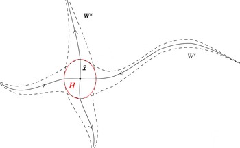
within the region in which the higher-order terms can be legitimately discarded. A situation associated with this reasoning is shown in figure 1, corresponding to a two-dimensional flow with one positive and one negative eigenvalue. The stable manifold
 $W^{s}$
of
 $\bar{\boldsymbol{x}}$
comes in along the eigenvector corresponding to the negative eigenvalue, and the unstable manifold
 $W^{u}$
is similarly associated with the positive eigenvalue. The neighbourhood
 $H$
is a conceptual region in which the linear approximation (2.2) is deemed valid. Once fluid elements are within
 $H$
, they will stretch exponentially, with a rate given by the positive eigenvalue, since they are pulled away by the unstable manifold. This will happen for fluid blobs that traverse the stable manifold as well, since, except for the (one-dimensional) part of the blob lying exactly on the stable manifold, the parts of the fluid element on its two sides will get pulled apart exponentially due to the unstable manifold. Now, since the linear approximation only works while in
 $H$
, there is no expectation of exponential stretching for instances when fluid elements are outside
 $H$
. However, fluid lying within the dashed envelope surrounding
 $W^{s}$
will eventually be within
 $H$
, and then will exponentially stretch. Similarly, fluid in the dashed envelope around
 $W^{u}$
will have experienced exponential stretching at some time in the past.
Hyperbolic neighbourhood
 $H$
(red) for a steady situation: fluid lying within
 $H$
experiences exponential stretching, while fluid elements within the dashed envelopes around the stable
 $W^{s}$
and unstable
 $W^{u}$
manifolds of the stagnation point
 $\bar{\boldsymbol{x}}$
will stretch once inside
 $H$
.

The region
 $H$
also has an underappreciated connection to both FTLE ridges and LCSs. Suppose the forward-time FTLE was computed for the situation pictured in figure 1. If this was done for a short time period
 $T$
, then parts of the stable manifold close to
 $\bar{\boldsymbol{x}}$
will emerge as large values of the FTLE field, since fluid elements there are within the immediate exponential stretching regime. However, if one computes for a larger time, then large FTLE values will also arise for parts of the stable manifold that are further away. In performing large
 $T$
calculations, another important factor is that it is only trajectories that are exactly on the stable manifold that will reside within
 $H$
forever after entering
 $H$
. These will therefore continue to incur exponential stretching forever, in contrast to other trajectories that will leave
 $H$
. Thus, if performing a forward-time FTLE calculation with large
 $T$
, the stable manifold will emerge as having anomalously large values of the FTLE and will be visible as a ridge. The sensitivity of FTLE ridges to the time
 $T$
over which the computation is performed is therefore directly related to whether that time would put fluid elements into
 $H$
or not, since it is only inside
 $H$
that exponential stretching occurs. Similarly, consider the definition of a repelling hyperbolic LCS of Haller (Reference Haller2011, Reference Haller2015). Exponential repulsion from the stable manifold will occur only once particles are within
 $H$
, and thus once again the method displays an intimate connection between the finite time over which the calculation is performed and whether this time would put certain particles into
 $H$
in its duration or not. In other words, the sensitivity of both FTLEs and hyperbolic LCSs to the finite time considered is linked to
 $H$
. We will explore the FTLE connection in more detail in § 3.3.
More realistically, the global flow will not be linear, and will contain several hyperbolic stagnation points. In this generic situation, fluid traversing the flow domain would have ‘exponential boosts’ to its stretching each time it went through a neighbourhood
 $H$
of a hyperbolic point. These neighbourhoods are therefore crucial to understanding the Lagrangian evolution of stretching.
2.2 Unsteady flows: hyperbolicity and its relationship to FTLEs/LCSs
When the flow is unsteady, we must generalize from hyperbolic fixed points (since in general there may no longer be any true fixed points) to hyperbolic trajectories. These objects are special solutions
 $\bar{\boldsymbol{x}}(t)$
of the Lagrangian equations of motion
 $$\begin{eqnarray}\displaystyle {\dot{x}}_{i}=u_{i}(\boldsymbol{x},t), & & \displaystyle\end{eqnarray}$$
for which the variational equation
 $$\begin{eqnarray}\displaystyle {\dot{y}}_{i}=y_{j}\frac{\unicode[STIX]{x2202}}{\unicode[STIX]{x2202}x_{j}}u_{i}(\bar{\boldsymbol{x}}(t),t) & & \displaystyle\end{eqnarray}$$
possesses an exponential dichotomy (Coppel Reference Coppel1978; Balasuriya Reference Balasuriya2012). Intuitively, this condition requires that there be one direction along which one can choose a material point at distance
 $\boldsymbol{y}(t)$
away from
 $\bar{\boldsymbol{x}}(t)$
such that
 $\boldsymbol{y}(t)$
decays exponentially quickly in forward time, and another direction along which
 $\boldsymbol{y}(t)$
decays exponentially in backward time. These conditions again imply the local existence of a stable and unstable manifold attached to the hyperbolic trajectory
 $\bar{\boldsymbol{x}}(t)$
, although unlike in the steady case, these manifolds evolve in time. The basic picture is something like that of figure 1, but the point
 $\bar{\boldsymbol{x}}$
is moving with time, as are the local directions of emanation of the stable/unstable manifolds and the manifolds themselves. Given these differences, it is clear that simply looking for instantaneous stagnation points need not capture hyperbolic stretching; nor do eigenvalues and eigenvectors provide information about the local behaviour (Balasuriya Reference Balasuriya2016b
).
In practice, finite-time hyperbolic trajectories tend to be determined in different ways depending on the particular method being used, and there is no universally agreed upon definition for them. If using FTLEs, they would be intersections of the forward- and backward-time FTLE ridges (Voth, Haller & Gollub Reference Voth, Haller and Gollub2002). We however note that this can be an ambiguous exercise, since defining exactly what makes a feature a ‘ridge’ is unclear. For example, how sharp must it be? Moreover, there is no guarantee that if one tracks an intersection point of ridges with time, it will be a trajectory of the flow (Haller Reference Haller2015). If using hyperbolic LCSs, they would be intersections of repelling and attracting LCSs. These characterizations mean that hyperbolic trajectories for finite-time flows may exist only for some times, and not others; although the trajectory of a given fluid element must be continuous in incompressible flow, it need not remain hyperbolic over its entire history. In particular, we can no longer say that a fluid element on the stable manifold will eventually experience exponential stretching: the time it would take for that fluid element to arrive near the hyperbolic trajectory may be longer than the hyperbolic trajectory exists. Fluid elements that are close to the hyperbolic trajectory will, however, experience the exponential stretching that is the signature of hyperbolicity. The dynamics of those fluid elements is therefore dominated by the hyperbolic trajectory, and determines its zone of influence in the fluid – which we shall refer to as its hyperbolic neighbourhood and label by
 $H(t)$
. This neighbourhood is likely to contain segments of the analogues of stable and unstable manifolds of the hyperbolic trajectory, as fluid elements on the manifolds and near to the hyperbolic trajectory will certainly feel their effects; but it will also likely contain fluid elements not on the manifolds but still close to the hyperbolic trajectory, in the region of the flow field where the streamlines are close to hyperbolæ. Thus, the hyperbolic neighbourhood is distinct from a simple estimate of the manifolds, due to its finite-time nature.
If the flow is steady, the directionality of the stretching incurred in forward time while within a hyperbolic neighbourhood is indicated by the direction of the unstable manifold in figure 1. In other words, this is the direction of the eigenspace spanned by the eigenvectors associated with eigenvalues with positive real part of the Jacobian matrix evaluated at the hyperbolic point
 $\bar{\boldsymbol{x}}$
. In backward time, the stretching occurs in the direction of the eigenspace associated with eigenvalues with negative real part. This directionality becomes less easy to define for unsteady flows since, just as the hyperbolic trajectory
 $\bar{\boldsymbol{x}}$
is moving with time, so are the directions of emanation of the stable/unstable manifolds. Formally, Balasuriya (Reference Balasuriya2016b
) shows that these time-varying directions can be characterized in terms of Oseledets spaces, or through exponential dichotomy projections, but these are difficult to use in most practical settings. Trajectories traversing
 $H(t)$
will experience exponential stretching instantaneously in these directions, but since they are changing with time, the accumulated stretching while within
 $H(t)$
cannot be encapsulated as being in a particular direction. Nevertheless, over a finite time interval, exponential separation between adjacent trajectories is to be expected while both are within
 $H(t)$
.
Before providing a definition as to how to determine
 $H(t)$
, we make the important observation that the variational equation (2.4) has a central role in determining either FTLEs or hyperbolic LCSs. If the finite time under consideration is from a time
 $t_{0}$
to a time
 $t_{0}+T$
, for example, let
 $\unicode[STIX]{x1D6F7}(\boldsymbol{x},t_{0},T)$
be the flow map that gives the location at time
 $t_{0}+T$
of the fluid element that was at
 $\boldsymbol{x}$
at time
 $t_{0}$
. It can be shown (Haller Reference Haller2011) that its gradient
 $$\begin{eqnarray}\displaystyle \unicode[STIX]{x1D621}_{ij}(T)=\frac{\unicode[STIX]{x2202}\unicode[STIX]{x1D6F7}_{i}}{\unicode[STIX]{x2202}x_{j}}(\boldsymbol{x},t_{0},T) & & \displaystyle\end{eqnarray}$$
is a fundamental matrix solution to the variational equation (2.4), in the sense that
 $$\begin{eqnarray}\displaystyle \frac{\text{d}}{\text{d}T}\unicode[STIX]{x1D621}_{ij}(T)=\unicode[STIX]{x1D621}_{kj}(T)\frac{\unicode[STIX]{x2202}}{\unicode[STIX]{x2202}x_{k}}u_{i}(\boldsymbol{x}(T),T);\quad \boldsymbol{x}(t_{0})=\boldsymbol{x}. & & \displaystyle\end{eqnarray}$$
The right Cauchy–Green strain tensor is formed from the contraction of the gradient of the flow map with itself, so that
 $$\begin{eqnarray}\displaystyle \unicode[STIX]{x1D60A}_{ij}(\boldsymbol{x},t_{0},T)=\frac{\unicode[STIX]{x2202}\unicode[STIX]{x1D6F7}_{k}}{\unicode[STIX]{x2202}x_{i}}\frac{\unicode[STIX]{x2202}\unicode[STIX]{x1D6F7}_{k}}{\unicode[STIX]{x2202}x_{j}}. & & \displaystyle\end{eqnarray}$$
If the largest eigenvalue of the Cauchy–Green tensor is
 $\unicode[STIX]{x1D706}_{max}$
, then the FTLE
 $\unicode[STIX]{x1D70E}$
is defined by (Shadden et al.
Reference Shadden, Lekien and Marsden2005)
 $$\begin{eqnarray}\displaystyle \unicode[STIX]{x1D70E}(\boldsymbol{x},t_{0},T)=\frac{1}{T}\ln (\sqrt{\unicode[STIX]{x1D706}_{max}(\boldsymbol{x},t_{0},T)}). & & \displaystyle\end{eqnarray}$$
We will in § 3.1 examine the FTLE in some more detail within the context of computation. The definition of hyperbolic LCSs (Haller Reference Haller2011, Reference Haller2015) also depends specifically on eigenvalues and eigenvectors of the Cauchy–Green tensor, or equivalently, on the singular values and vectors of
 $\unicode[STIX]{x1D655}$
, the fundamental matrix solution of the variational equation. The crucial observation is that both FTLEs and hyperbolic LCSs therefore depend on a solution to the variational equation (2.4), which is only valid if the higher-order nonlinear terms are discarded. In other words, conclusions arising from these definitions are only reasonable in a small enough neighbourhood travelling along with the trajectory that is being examined.
2.3 Hyperbolic neighbourhoods: dominance of linearity
How, then, does one determine a hyperbolic neighbourhood? The key to our method is the requirement that it is precisely the region in space around the hyperbolic trajectory, where the linearized flow near the hyperbolic trajectory gives a good approximation to the actual flow. To see how this condition helps us to estimate
 $H(t)$
, let us recall how (2.4) is obtained. First, we let
 $\boldsymbol{x}(t)=\bar{\boldsymbol{x}}(t)+\boldsymbol{y}(t)$
, where
 $\boldsymbol{y}(t)$
is the deviation away from the hyperbolic trajectory
 $\bar{\boldsymbol{x}}(t)$
. Inserting into (2.3), we obtain
 $$\begin{eqnarray}\displaystyle \dot{\bar{x}}_{i}+{\dot{y}}_{i}=u_{i}(\bar{\boldsymbol{x}}+\boldsymbol{y},t)=u_{i}(\bar{\boldsymbol{x}},t)+y_{j}\frac{\unicode[STIX]{x2202}}{\unicode[STIX]{x2202}x_{j}}u_{i}(\bar{\boldsymbol{x}},t)+O(|\boldsymbol{y}|^{2}), & & \displaystyle\end{eqnarray}$$
where the second equality follows from Taylor expanding the velocity field. Now, if we assume that the variation
 $\boldsymbol{y}(t)$
is very small at time
 $t$
so that the second fluid element is very close to the hyperbolic trajectory, we can keep only terms up to
 $O(|\boldsymbol{y}|)$
, thereby recovering (2.4). This derivation, however, also allows us to bound the error introduced by keeping only the first-order terms. Since
 $\bar{\boldsymbol{x}}(t)$
is itself a Lagrangian trajectory, we can also write
 $$\begin{eqnarray}\displaystyle {\dot{y}}_{i}=u_{i}(\bar{\boldsymbol{x}}+\boldsymbol{y},t)-\dot{\bar{x}}_{i}=u_{i}(\bar{\boldsymbol{x}}+\boldsymbol{y},t)-u_{i}(\bar{\boldsymbol{x}},t), & & \displaystyle\end{eqnarray}$$
where we have made no approximations. The error in the variational approximation is then the difference between this equation and the variational equation. Now, above we described the hyperbolic neighbourhood
 $H(t)$
as being the region around
 $\bar{\boldsymbol{x}}(t)$
in which its hyperbolic character is preserved so that the flow stretches exponentially. We can now make this notion more precise by defining
 $H(t)$
to be the region around
 $\bar{\boldsymbol{x}}(t)$
in which the replacement of (2.10) by (2.4) is valid – in other words, the region in which the approximation error is small when compared with the retained terms. This condition can be quantified by
 $$\begin{eqnarray}\displaystyle \left|y_{j}\frac{\unicode[STIX]{x2202}}{\unicode[STIX]{x2202}x_{j}}u_{i}(\bar{\boldsymbol{x}}(t),t)\right|\gg \left|u_{i}(\bar{\boldsymbol{x}}(t)+\boldsymbol{y},t)-u_{i}(\bar{\boldsymbol{x}}(t),t)-y_{j}\frac{\unicode[STIX]{x2202}}{\unicode[STIX]{x2202}x_{j}}u_{i}(\bar{\boldsymbol{x}}(t),t)\right|. & & \displaystyle\end{eqnarray}$$
This condition requires that the estimate of the velocity difference between points
 $\bar{\boldsymbol{x}}+\boldsymbol{y}$
and
 $\bar{\boldsymbol{x}}$
by the velocity gradient at
 $\bar{\boldsymbol{x}}$
alone is very good – or, in other words, that the flow is very close to the linear flow at the hyperbolic trajectory. As long as the velocity gradient at
 $\bar{\boldsymbol{x}}(t)$
has no purely imaginary eigenvalues, this condition will be achievable for some non-empty set.
Definition 1 (Hyperbolic neighbourhood (HN)).
The hyperbolic neighbourhood
 $H(t)$
of a hyperbolic trajectory
 $\bar{\boldsymbol{x}}(t)$
is the set
 $$\begin{eqnarray}\displaystyle H(t):=\left\{\bar{\boldsymbol{x}}(t)+\boldsymbol{y}:\left|y_{j}\frac{\unicode[STIX]{x2202}}{\unicode[STIX]{x2202}x_{j}}u_{i}(\bar{\boldsymbol{x}}(t),t)\right|>E\left|u_{i}(\bar{\boldsymbol{x}}(t)+\boldsymbol{y},t)-u_{i}(\bar{\boldsymbol{x}}(t),t)-y_{j}\frac{\unicode[STIX]{x2202}}{\unicode[STIX]{x2202}x_{j}}u_{i}(\bar{\boldsymbol{x}}(t),t)\right|\right\}\!, & & \displaystyle \nonumber\\ \displaystyle & & \displaystyle\end{eqnarray}$$
which depends on a constant
 $E\geqslant 1$
.
We have introduced a constant
 $E\geqslant 1$
that explicitly allows us to specify how accurate we require the linear approximation to be. In general, as
 $E$
is increased, the size of
 $H(t)$
will decrease (though there are exceptions, which we shall address in § 3.3) – and thus for very large values of
 $E$
,
 $H(t)$
may be unmeasurable from experiments or observations where the spatial resolution of the velocity field is always finite. We therefore expect that some tuning of
 $E$
will likely be necessary in these cases so as to draw meaningful conclusions. We will show, via analytical examples, that making a choice of
 $E$
is essentially equivalent to making a choice of a cutoff exponential stretching rate, and that the results obtained by this process are not hugely sensitive to
 $E$
.
We remark that our definition of hyperbolic neighbourhoods (HNs) is quite different from the concept of ‘LCS cores’ introduced by Olascoaga & Haller (Reference Olascoaga and Haller2012) that attempt to delimit the most important segments of the attracting/repelling hyperbolic LCSs in two-dimensional flows. Having identified a hyperbolic trajectory and its attached attracting LCS curve, they follow the curve until the strain rate towards it reverses direction, and clip the attracting LCS at that point. In computing the strain rate, they use quantities derived from the linearized flow, essentially the variational equation at each point on the LCS. By doing this, they are able to clip an attracting and a repelling LCS near a hyperbolic trajectory, with the understanding that the flow topology nearby is like hyperbolæ. This process identifies two intersecting curve segments, and not a region. Moreover, the method of Olascoaga & Haller (Reference Olascoaga and Haller2012) does not seek to check when a linear approximation is legitimate. Indeed, the process uses strictly linearized flow on the structures. In contrast, our hyperbolic neighbourhoods directly investigate the concept of linearity, and thereby exponential stretching.
We have already mentioned that exponential behaviour cannot be strictly verified in finite-time flows, since any function can be bounded by an exponential over a finite time interval. We have avoided this difficulty by directly searching for linearity in the flow field, which drives ‘instantaneous exponential stretching’ in an intuitive sense. While this latter concept cannot be defined clearly, the former can be quantified, and leads to our definition of hyperbolic neighbourhoods.
In thinking in terms of hyperbolic neighbourhoods, we have also highlighted some aspects of FTLEs/LCSs that are often hidden. These quantities are usually calculated at a time
 $t_{0}$
, with computations being done until a time
 $t_{0}+T$
, for some fixed
 $T$
. Thus,
 $T$
might be thought of as the time period over which the relevant structures are important according to whatever definition one is using. In test examples such as the double gyre (Shadden et al.
Reference Shadden, Lekien and Marsden2005), hyperbolicity lasts over any time period chosen, and thus the choice of
 $T$
(apart from not being too large or small) usually does not affect outputs significantly. The transitory nature of hyperbolic structures in realistic flows associated with finite-time data, however, makes the choice of
 $T$
crucial. Referring back to figure 1, consider fluid elements chosen near
 $W^{s}$
far to the right at time
 $t_{0}$
, but imagine that this is a finite-time, unsteady situation. If the time
 $T$
is such that (i) the hyperbolicity of
 $\bar{\boldsymbol{x}}$
disappears during this time, (ii) these elements have not entered
 $H$
by time
 $t_{0}+T$
or (iii) the fluid elements passed quickly though
 $H$
and are well away from
 $H$
by time
 $t_{0}+T$
, then the influence of the hyperbolic neighbourhood may not be noticed at all. These considerations can make the methodology being used highly sensitive to
 $T$
. This sensitivity is embraced by our concept of hyperbolic neighbourhoods, since they are able to identify, at each time
 $t$
between
 $t_{0}$
and
 $t_{0}+T$
, the parts of space that experience hyperbolicity, thereby enabling a broader picture of how to instantaneously segment the flow domain into regions in which the flow behaves ‘differently’. It must also be emphasized that our method works even for compressible flows with general time dependence, and in any dimension, assuming the hyperbolic trajectories can be determined.
Our definition of hyperbolic neighbourhoods is also objective (Truesdell & Noll Reference Truesdell and Noll2004; Haller Reference Haller2015; Peacock, Froyland & Haller Reference Peacock, Froyland and Haller2015), in that they are invariant under affine coordinate transformations of the form
 $$\begin{eqnarray}\displaystyle z_{i}=\unicode[STIX]{x1D618}_{ij}(t)x_{j}+b_{i}(t), & & \displaystyle\end{eqnarray}$$
where
 $\boldsymbol{b}(t)$
is an arbitrary vector and
 $\unicode[STIX]{x1D618}_{ij}(t)$
is an orthogonal tensor. The invariance occurs since the
 $t$
in (2.12) appears only as a parameter (there are no
 $t$
-derivatives, for example). The hyperbolic trajectory location would be at
 $\bar{z}_{i}(t)=\unicode[STIX]{x1D618}_{ij}(t)\bar{x}_{j}(t)+b_{i}(t)$
in the transformed frame, and if
 $\boldsymbol{w}$
is the deviation from this, we have
 $w_{i}=\unicode[STIX]{x1D618}_{ij}(t)y_{j}$
as the relationship between the local deviations in the two reference frames. Thus, if
 $\boldsymbol{U}(\boldsymbol{z},t)$
is the velocity field as represented in the
 $\boldsymbol{z}$
-frame, the linear term in the
 $\boldsymbol{z}$
-frame takes the form
 $$\begin{eqnarray}\displaystyle w_{j}\frac{\unicode[STIX]{x2202}}{\unicode[STIX]{x2202}z_{j}}U_{i}(\bar{\boldsymbol{z}}(t),t)=(Q_{jk}(t)y_{k})\left(\frac{\unicode[STIX]{x2202}}{\unicode[STIX]{x2202}x_{\ell }}u_{i}(\bar{\boldsymbol{x}}(t),t)Q_{\ell j}^{-1}(t)\right)=y_{j}\frac{\unicode[STIX]{x2202}}{\unicode[STIX]{x2202}x_{j}}u_{i}(\bar{\boldsymbol{x}}(t),t), & & \displaystyle\end{eqnarray}$$
which is invariant. The other terms appearing in (2.12) involve the difference between the velocity at two points, which is also invariant under the transformation, and thus – assuming that an objective criterion has been used in identifying the hyperbolic trajectories – hyperbolic neighbourhoods are objective.
We note that we have outlined here a method for determining the hyperbolic neighbourhood associated with a particular hyperbolic trajectory – but not a method for finding the hyperbolic trajectory itself. In general, finding such objects can be difficult, but there are also analytical (Balasuriya Reference Balasuriya2011) and numerical methods (Dellnitz & Junge Reference Dellnitz and Junge2002; Balasuriya & Padberg-Gehle Reference Balasuriya and Padberg-Gehle2014) as alternatives to the curve intersection ideas associated with FTLEs and LCSs. A tractable method must be chosen for general experimental or observational data, as we outline in § 4.2.
3 Analytical examples
To build intuition for what these hyperbolic neighbourhoods mean, we consider here several analytical examples where the hyperbolic neighbourhoods can be explicitly determined. We will demonstrate the fact that trajectories entering an HN display boosts to their instantaneous exponential stretching rate, which diminishes as they leave the HN. The residence time within HNs will be established to be correlated to the long-term stretching rates as identifiable via FTLEs. The connection between the factor
 $E$
in the definition of HNs and a ‘threshold stretching rate’ will be qualitatively and quantitatively established through these examples. Furthermore, we will show why some instances in which FTLEs provide unexpected results (Haller Reference Haller2011) can be attributed directly to the geometry of the HNs.
3.1 Steady Taylor–Green flow
The well-known steady Taylor–Green flow is defined by the streamfunction
 $$\begin{eqnarray}\displaystyle \unicode[STIX]{x1D713}(\boldsymbol{x})=\cos x_{1}\cos x_{2}, & & \displaystyle\end{eqnarray}$$
which gives the velocity field as
 $$\begin{eqnarray}\displaystyle \left.\begin{array}{@{}c@{}}\displaystyle {\dot{x}}_{1}=-\!\cos x_{1}\sin x_{2}\\ \displaystyle {\dot{x}}_{2}=\sin x_{1}\cos x_{2}.\end{array}\right\} & & \displaystyle\end{eqnarray}$$
Since this flow is periodic in both directions, it has an infinite number of critical points (Ouellette & Gollub Reference Ouellette and Gollub2007). Let us focus on the critical point
 $\bar{\boldsymbol{x}}=(\unicode[STIX]{x03C0}/2,\unicode[STIX]{x03C0}/2)$
, which is hyperbolic; and note that, as this is a steady flow, this point is also a hyperbolic trajectory. For this flow, the velocity gradient is given by
 $$\begin{eqnarray}\displaystyle \unicode[STIX]{x1D735}\boldsymbol{u}=\left(\begin{array}{@{}cc@{}}\displaystyle \sin x_{1}\sin x_{2} & -\!\cos x_{1}\cos x_{2}\\ \displaystyle \cos x_{1}\cos x_{2} & -\!\sin x_{1}\sin x_{2}\end{array}\right), & & \displaystyle\end{eqnarray}$$
and so we have
 $$\begin{eqnarray}\displaystyle y_{j}\frac{\unicode[STIX]{x2202}}{\unicode[STIX]{x2202}x_{j}}u_{i}(\bar{\boldsymbol{x}},t)=\left(\begin{array}{@{}cc@{}}1 & 0\\ 0 & -1\end{array}\right)\left(\begin{array}{@{}c@{}}y_{1}\\ y_{2}\end{array}\right)=\left(\begin{array}{@{}c@{}}y_{1}\\ -y_{2}\end{array}\right). & & \displaystyle\end{eqnarray}$$
Therefore,
 $$\begin{eqnarray}\displaystyle \boldsymbol{u}(\bar{\boldsymbol{x}}+\boldsymbol{y},t)-\boldsymbol{u}(\bar{\boldsymbol{x}},t)-\unicode[STIX]{x1D735}\boldsymbol{u}(\bar{\boldsymbol{x}},t)\boldsymbol{\cdot }\boldsymbol{y} & = & \displaystyle \left(\begin{array}{@{}c@{}}\displaystyle -\!\cos \left(\frac{\unicode[STIX]{x03C0}}{2}+y_{1}\right)\sin \left(\frac{\unicode[STIX]{x03C0}}{2}+y_{2}\right)\\ \displaystyle \sin \left(\frac{\unicode[STIX]{x03C0}}{2}+y_{1}\right)\cos \left(\frac{\unicode[STIX]{x03C0}}{2}+y_{2}\right)\end{array}\right)-\left(\begin{array}{@{}c@{}}y_{1}\\ -y_{2}\end{array}\right)\nonumber\\ \displaystyle & = & \displaystyle \left(\begin{array}{@{}c@{}}\sin y_{1}\cos y_{2}-y_{1}\\ -\!\cos y_{1}\sin y_{2}+y_{2}\end{array}\right).\end{eqnarray}$$
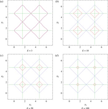
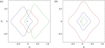
Hyperbolic neighbourhoods (red solid lines) for the steady Taylor–Green flow, as defined by (3.6), for several values of
 $E$
. The stable/unstable manifold connections between the hyperbolic points are shown with green horizontal and vertical lines. For comparison, the blue dashed lines show the regions that would be identified as hyperbolic based on the instantaneous Okubo–Weiss criterion (3.8).

The hyperbolic neighbourhood associated with a hyperbolic point
 $\bar{\boldsymbol{x}}=(\bar{x}_{1},\bar{x}_{2})$
is therefore
 $$\begin{eqnarray}\displaystyle H=\{(\bar{x}_{1}+y_{1},\bar{x}_{2}+y_{2}):y_{1}^{2}+y_{2}^{2}>E^{2}[(\sin y_{1}\cos y_{2}-y_{1})^{2}+(-\!\cos y_{1}\sin y_{2}+y_{2})^{2}]\}, & & \displaystyle \nonumber\\ \displaystyle & & \displaystyle\end{eqnarray}$$
where for convenience we have squared both sides of the inequality in (2.12). This neighbourhood is shown in figure 2, along with the hyperbolic neighbourhoods associated with the hyperbolic points at
 $(\unicode[STIX]{x03C0}/2,5\unicode[STIX]{x03C0}/2)$
,
 $(5\unicode[STIX]{x03C0}/2,\unicode[STIX]{x03C0}/2)$
, and
 $(5\unicode[STIX]{x03C0}/2,5\unicode[STIX]{x03C0}/2)$
. For comparison, we also show the regions that would be identified as hyperbolic based on the Okubo–Weiss criterion (Okubo Reference Okubo1970; Weiss Reference Weiss1991); that is, regions that satisfy
 $$\begin{eqnarray}\displaystyle \det \unicode[STIX]{x1D735}\boldsymbol{u}<0, & & \displaystyle\end{eqnarray}$$
or
 $$\begin{eqnarray}\displaystyle -\!\sin ^{2}x_{1}\sin ^{2}x_{2}+\cos ^{2}x_{1}\cos ^{2}x_{2}<0 & & \displaystyle\end{eqnarray}$$
in this case. For this flow, the HNs with
 $E=3$
are quite similar (although not identical) to those regions predicted to be hyperbolic based on the Okubo–Weiss criterion. This similarity is reasonable, since, for steady flows, the Okubo–Weiss criterion is fairly effective at indicating hyperbolic regions; objections to it are primarily concerned with the relative time scales over which the velocity gradient and the vorticity gradient evolve (Rivera, Aluie & Ecke Reference Rivera, Aluie and Ecke2014). As
 $E$
is increased, the HNs become smaller. We can think of
 $E$
as being our measure for how closely we require linearity.
An interesting observation from the nature of the HNs in figure 2 is that they exhibit a weak elongation in the direction of the stable and unstable manifolds; they ‘stick out’ slightly in those directions. The intuition for this observation is that the exponential stretching is exact in the direction of the stable/unstable manifolds local to the hyperbolic point and identifiable with the eigenvalue of the linearized velocity gradient matrix. The direction of the manifold is in fact the corresponding eigenvector direction. Slightly off a stable/unstable manifold, while the behaviour is certainly dominated by the eigenvalue associated with this nearby manifold, there is also a contribution to the stretching arising from the other eigenvalue, which has the opposite sign. This, then, diminishes the stretching in comparison to being exactly on the manifold. Thus, the region of dominance of linearity tends to push out along the stable and unstable manifold directions in this case. As we shall see later, there are instances in which this generic behaviour does not occur, in what we shall identify to be degenerate HNs.
Next, we verify our claim that the exponential stretching rate within HNs is anomalously larger than outside HNs. To do so, consider a pair of points
 $\unicode[STIX]{x1D6FC}^{1}$
and
 $\unicode[STIX]{x1D6FD}^{1}$
at an initial time
 $t_{0}$
, located close to
 $(\unicode[STIX]{x03C0}/2,\unicode[STIX]{x03C0})$
, i.e. near the stable manifold of
 $(\unicode[STIX]{x03C0}/2,\unicode[STIX]{x03C0}/2)$
. Let
 $\unicode[STIX]{x1D6F7}_{\unicode[STIX]{x1D6FC}}^{1}(t)$
and
 $\unicode[STIX]{x1D6F7}_{\unicode[STIX]{x1D6FD}}^{1}(t)$
be trajectories of (3.2), as a function of time, that satisfy
 $\unicode[STIX]{x1D6F7}_{\unicode[STIX]{x1D6FC}}^{1}(t_{0})=\unicode[STIX]{x1D6FC}^{1}$
and
 $\unicode[STIX]{x1D6F7}_{\unicode[STIX]{x1D6FD}}^{1}(t_{0})=\unicode[STIX]{x1D6FD}^{1}$
. In this vein, imagine many pairs of trajectories
 $\unicode[STIX]{x1D6F7}_{\unicode[STIX]{x1D6FC}}^{i}(t)$
and
 $\unicode[STIX]{x1D6F7}_{\unicode[STIX]{x1D6FD}}^{i}(t)$
that satisfy
 $\unicode[STIX]{x1D6F7}_{\unicode[STIX]{x1D6FC}}^{i}(t_{0})=\unicode[STIX]{x1D6FC}^{i}$
and
 $\unicode[STIX]{x1D6F7}_{\unicode[STIX]{x1D6FD}}^{i}(t_{0})=\unicode[STIX]{x1D6FD}^{i}$
. If
 $\unicode[STIX]{x1D706}^{i}(t)$
is the instantaneous measure of the exponential rate of stretching of the distance between the trajectories
 $\unicode[STIX]{x1D6F7}_{\unicode[STIX]{x1D6FC}}^{i}(t)$
and
 $\unicode[STIX]{x1D6F7}_{\unicode[STIX]{x1D6FD}}^{i}(t)$
at time
 $t$
, we can think of approximating it via
 $$\begin{eqnarray}\displaystyle e^{\unicode[STIX]{x1D706}^{i}(t)\unicode[STIX]{x0394}t}=\frac{|\unicode[STIX]{x1D6F7}_{\unicode[STIX]{x1D6FC}}^{i}(t+\unicode[STIX]{x0394}t)-\unicode[STIX]{x1D6F7}_{\unicode[STIX]{x1D6FD}}^{i}(t+\unicode[STIX]{x0394}t)|}{|\unicode[STIX]{x1D6F7}_{\unicode[STIX]{x1D6FC}}^{i}(t)-\unicode[STIX]{x1D6F7}_{\unicode[STIX]{x1D6FD}}^{i}(t)|} & & \displaystyle\end{eqnarray}$$
over a short time interval
 $[t,t+\unicode[STIX]{x0394}t]$
. Thus, we can computationally recover the instantaneous exponential stretching rate for a pair of trajectories starting at
 $\unicode[STIX]{x1D6FC}^{i}$
and
 $\unicode[STIX]{x1D6FD}^{i}$
as
 $$\begin{eqnarray}\displaystyle \unicode[STIX]{x1D706}^{i}(t)=\frac{1}{\unicode[STIX]{x0394}t}\ln \frac{|\unicode[STIX]{x1D6F7}_{\unicode[STIX]{x1D6FC}}^{i}(t+\unicode[STIX]{x0394}t)-\unicode[STIX]{x1D6F7}_{\unicode[STIX]{x1D6FD}}^{i}(t+\unicode[STIX]{x0394}t)|}{|\unicode[STIX]{x1D6F7}_{\unicode[STIX]{x1D6FC}}^{i}(t)-\unicode[STIX]{x1D6F7}_{\unicode[STIX]{x1D6FD}}^{i}(t)|}. & & \displaystyle\end{eqnarray}$$
We will momentarily use this measure – a pairwise instantaneous stretching rate – to compute stretching rates for the Taylor–Green flow. First, though, we establish a connection between it and FTLEs. Imagine that we start at time
 $t_{0}$
with a pair of points
 $\unicode[STIX]{x1D6FC}^{i}$
and
 $\unicode[STIX]{x1D6FD}^{i}$
, and track the trajectories
 $\unicode[STIX]{x1D6F7}_{\unicode[STIX]{x1D6FC}}^{i}$
and
 $\unicode[STIX]{x1D6F7}_{\unicode[STIX]{x1D6FD}}^{i}$
numerically until time
 $t_{0}+T$
, thereby obtaining information at discrete times
 $t_{0}+j\unicode[STIX]{x0394}t$
,
 $j=0,1,2,\ldots ,n$
, where
 $n\unicode[STIX]{x0394}t=T$
. Thus, the average accumulated instantaneous stretching over the full finite time period is
 $$\begin{eqnarray}\displaystyle \unicode[STIX]{x1D6EC}^{i}(t_{0},t_{0}+T) & := & \displaystyle \frac{1}{n}\mathop{\sum }_{j=0}^{n-1}\frac{1}{\unicode[STIX]{x0394}t}\ln \frac{|\unicode[STIX]{x1D6F7}_{\unicode[STIX]{x1D6FC}}^{i}(t_{j}+\unicode[STIX]{x0394}t)-\unicode[STIX]{x1D6F7}_{\unicode[STIX]{x1D6FD}}^{i}(t_{j}+\unicode[STIX]{x0394}t)|}{|\unicode[STIX]{x1D6F7}_{\unicode[STIX]{x1D6FC}}^{i}(t_{j})-\unicode[STIX]{x1D6F7}_{\unicode[STIX]{x1D6FD}}^{i}(t_{j})|}\nonumber\\ \displaystyle & = & \displaystyle \frac{1}{n\unicode[STIX]{x0394}t}\ln \frac{|\unicode[STIX]{x1D6F7}_{\unicode[STIX]{x1D6FC}}^{i}(t_{0}+T)-\unicode[STIX]{x1D6F7}_{\unicode[STIX]{x1D6FD}}^{i}(t_{0}+T)|}{|\unicode[STIX]{x1D6F7}_{\unicode[STIX]{x1D6FC}}^{i}(t_{0})-\unicode[STIX]{x1D6F7}_{\unicode[STIX]{x1D6FD}}^{i}(t_{0})|}\nonumber\\ \displaystyle & = & \displaystyle \frac{1}{T}\ln \frac{|\unicode[STIX]{x1D6F7}_{\unicode[STIX]{x1D6FC}}^{i}(t_{0}+T)-\unicode[STIX]{x1D6F7}_{\unicode[STIX]{x1D6FD}}^{i}(t_{0}+T)|}{|\unicode[STIX]{x1D6F7}_{\unicode[STIX]{x1D6FC}}^{i}(t_{0})-\unicode[STIX]{x1D6F7}_{\unicode[STIX]{x1D6FD}}^{i}(t_{0})|}.\end{eqnarray}$$
If thinking of
 $\unicode[STIX]{x1D6FC}^{i}$
as a fixed initial location at time
 $t_{0}$
, the forward FTLE field at
 $\unicode[STIX]{x1D6FC}^{i}$
, given in terms of the Cauchy–Green tensor by (2.8), has the equivalent form (Shadden et al.
Reference Shadden, Lekien and Marsden2005; Balasuriya Reference Balasuriya2012; Haller Reference Haller2015)
 $$\begin{eqnarray}\displaystyle \unicode[STIX]{x1D70E}(\unicode[STIX]{x1D6FC}^{i},t_{0},T)=\frac{1}{T}\ln \sup _{\unicode[STIX]{x1D6FD}^{i}}\frac{|\unicode[STIX]{x1D6F7}_{\unicode[STIX]{x1D6FC}}^{i}(t_{0}+T)-\unicode[STIX]{x1D6F7}_{\unicode[STIX]{x1D6FD}}^{i}(t_{0}+T)|}{|\unicode[STIX]{x1D6F7}_{\unicode[STIX]{x1D6FC}}^{i}(t_{0})-\unicode[STIX]{x1D6F7}_{\unicode[STIX]{x1D6FD}}^{i}(t_{0})|}, & & \displaystyle\end{eqnarray}$$
where the supremum over
 $\unicode[STIX]{x1D6FD}^{i}$
indicates that one takes initial locations
 $\unicode[STIX]{x1D6FD}^{i}$
in all possible directions from
 $\unicode[STIX]{x1D6FC}^{i}$
, but then chooses the direction such that the ratio of expansion above is maximized. Indeed, Samelson (Reference Samelson2013) argues that the FTLE defined in (3.12) might be more naturally interpreted in the fluid dynamics context as a finite-time Lagrangian strain; to avoid confusion as to exactly what ‘strain’ may mean, we offer the additional modification that perhaps it should be thought of as a finite-time Lagrangian stretching. In any case, the connection between the average accumulated stretching (3.11) and the FTLE (3.12) is clear: these are proportional to one another if
 $\unicode[STIX]{x1D6FD}^{i}$
is chosen infinitesimally closely in the direction in which the FTLE at
 $\unicode[STIX]{x1D6FC}^{i}$
is maximized. Therefore, the instantaneous stretching rate definition (3.10) we will use for numerical evaluation is strongly connected to the FTLE; loosely speaking, its accumulated effects lead to the FTLE over a finite time interval. (Though the FTLE does have the added ‘supremum over all directions’ as part of its definition, whereas (3.10) is a pairwise stretching measure.)
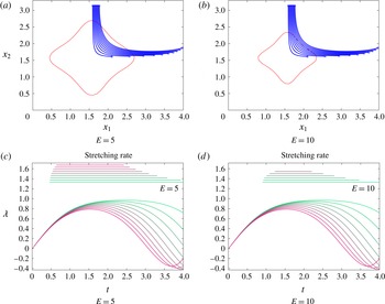
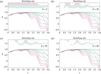
The flow of trajectories in comparison with the HN (a,b) with the initial seedings shown by crosses and the final location by circles, and the computed instantaneous stretching rate (3.10) for the Taylor–Green flow (c,d) at different
 $E$
values, with the range over which a particular coloured trajectory is within the HN indicated by the lines at the top.

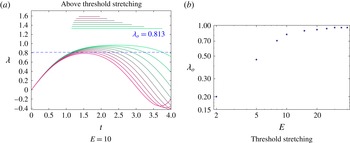
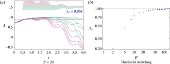
(a) The stretching rates of figure 3(b), but with the range over which
 $\unicode[STIX]{x1D706}$
is larger than a threshold value
 $\unicode[STIX]{x1D706}_{o}$
indicated by the lines at the top of the figure. (b)
 $\unicode[STIX]{x1D706}_{o}$
values as functions of
 $E$
plotted on logarithmic axes for the Taylor–Green flow, chosen by minimizing (3.13), with identical parameter values as for figure 3 being used.

With these connections understood, we can now return to the Taylor–Green flow and evaluate how the stretching between trajectories is impacted by being within HNs. We seed a collection of fluid particles (blue xs) as shown in figure 3(a,b), which will pass into the HN (shown in red) during our time of integration. For each adjacent pair of initial particle locations, we show in the bottom panels how the instantaneous stretching rate (3.10) varies. Each colour corresponds to a pair of trajectories. We deem that a pair of trajectories is within the HN centred at
 $(\unicode[STIX]{x03C0}/2,\unicode[STIX]{x03C0}/2)$
if their midpoint is within the HN at that time. The range of time over which a particular pair of trajectories is within the HN is indicated by the line of identical colour towards the top of the figures. All trajectories initially have small values of
 $\unicode[STIX]{x1D706}$
, since they are outside the HN. As they approach the HN, the value of
 $\unicode[STIX]{x1D706}$
increases appreciably, thereby demonstrating that strong exponential stretching is occurring. If
 $E=5$
, the HN is chosen to be fairly large, and if
 $E=10$
, it is smaller (and shown in figure 2
b). When
 $E$
is larger, a smaller number of trajectory pairs are indicated as being within an HN, and moreover are within an HN for a shorter time than when
 $E$
is smaller. Thus, figure 3 validates very clearly our claim that trajectories entering HNs experience a boost in their exponential stretching, and lose it as they leave.
The time of residence – as indicated by the lengths of the lines at the top of figure 3 – is clearly linked to when
 $\unicode[STIX]{x1D706}$
is large in the corresponding curve below. In other words, if the stretching curves were cut off below a certain threshold, it would appear that the time ranges at the top of the figure would be obtained. We investigate this quantitatively in figure 4. For a given
 $E$
value, we determine the stretching threshold
 $\unicode[STIX]{x1D706}_{o}$
such that if keeping only time values for which the stretching rates are above
 $\unicode[STIX]{x1D706}_{o}$
in figure 3, we recover ‘close to’ the time range within the HN as reflected by the time-range lines at the top of figure 3. We define this closeness as follows. Let
 $\text{HN}^{i}(t_{j})$
be the indicator functions as to whether trajectory pair
 $i$
is within the HN at time
 $t_{j}$
, i.e.
 $\text{HN}^{i}(t_{j})=1$
if the midpoint is within HN at time
 $t_{j}$
and
 $0$
if not. Let
 $I^{i}(t_{j})$
be an indicator function as to whether
 $\unicode[STIX]{x1D706}(t_{j})>\unicode[STIX]{x1D706}_{0}$
at time
 $t_{j}$
. Then, we define the discrepancy between these by
 $$\begin{eqnarray}\displaystyle \unicode[STIX]{x1D716}(\unicode[STIX]{x1D706}_{o})=\frac{\unicode[STIX]{x0394}t}{mT}\mathop{\sum }_{j=0}^{n-1}\mathop{\sum }_{i=1}^{m}|\text{HN}^{i}(t_{j})-I^{i}(t_{j})|, & & \displaystyle\end{eqnarray}$$
where there are
 $m$
trajectory pairs considered. Note that this is essentially an
 $\text{L}^{1}$
-norm, suitably averaged over time and number of pairs of trajectories. By sweeping over choices of
 $\unicode[STIX]{x1D706}_{o}$
, we determine the value of
 $\unicode[STIX]{x1D706}_{o}$
that minimizes
 $\unicode[STIX]{x1D716}(\unicode[STIX]{x1D706}_{o})$
. In figure 4(a), we show the computed range functions
 $I^{i}(t)$
at the top of the figure for
 $E=10$
, for a direct comparison with figure 3(b) (in which the range functions at the top of the figure correspond to
 $\text{HN}^{i}(t)$
). Thus, choosing an HN with
 $E=10$
is very similar to choosing a threshold stretching rate of
 $\unicode[STIX]{x1D706}_{o}=0.813$
, which is shown by the dashed blue line in figure 4(a). In other words, this is the choice that makes the ‘being within HN’ and ‘being above the stretching threshold’ conditions similar. In this way, we can find the appropriate threshold stretching
 $\unicode[STIX]{x1D706}_{o}$
corresponding to different
 $E$
values, and present this information in figure 4(b). As
 $E$
gets larger the variation of
 $\unicode[STIX]{x1D706}_{o}$
slows; this corresponds to the statement that as one approaches the hyperbolic trajectory arbitrarily closely, the stretching rate is effectively the stretching rate of the hyperbolic trajectory. Theoretically we would expect this value to approach
 $1$
, which is the unstable eigenvalue associated with the stagnation point
 $(\unicode[STIX]{x03C0}/2,\unicode[STIX]{x03C0}/2)$
. Obtaining this numerically in the limit
 $E\rightarrow \infty$
requires continually refining the spatial resolution, since as
 $E\rightarrow \infty$
, the size of the HN itself approaches zero, but must remain resolved for these computations to be performed. Figure 4(b) therefore enables a quantitative evaluation of how the factor
 $E$
in the definition of the HN is related to how the exponential stretching within the HN is close to that of its core hyperbolic trajectory.
3.2 Duffing equation
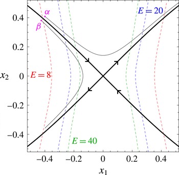
Hyperbolic neighbourhoods (boundaries shown with dashed curves) for the Duffing equation, as computed from (3.18), for
 $E=8$
(red),
 $20$
(blue) and
 $40$
(green). The stable and unstable manifolds of the origin are shown by the thick black curves, and the thin curves show how two different trajectories, starting at locations
 $\unicode[STIX]{x1D6FC}$
and
 $\unicode[STIX]{x1D6FD}$
, traverse the HNs.

As a second example, consider the steady, unforced Duffing equation (Wiggins Reference Wiggins1992; Balasuriya Reference Balasuriya2011)
 $$\begin{eqnarray}\displaystyle \left.\begin{array}{@{}c@{}}\displaystyle {\dot{x}}_{1}=x_{2}\\ \displaystyle {\dot{x}}_{2}=x_{1}-x_{1}^{3}\end{array}\right\} & & \displaystyle\end{eqnarray}$$
which has a hyperbolic fixed point at the origin, to which is attached one-dimensional stable and unstable manifolds (see figure 5). Since this is again a steady (autonomous) system, the corresponding hyperbolic trajectory is simply
 $(0,0,t)$
for all
 $t$
; moreover, the hyperbolic neighbourhood
 $H(t)$
will also be the same for all
 $t$
. The velocity gradient is easily calculated to be
 $$\begin{eqnarray}\displaystyle \unicode[STIX]{x1D735}\boldsymbol{u}=\left(\begin{array}{@{}cc@{}}0 & 1\\ 1-3x_{1}^{2} & 0\end{array}\right), & & \displaystyle\end{eqnarray}$$
from which we obtain
 $$\begin{eqnarray}\displaystyle y_{j}\frac{\unicode[STIX]{x2202}}{\unicode[STIX]{x2202}x_{j}}u_{i}(\bar{\boldsymbol{x}},t)=\left(\begin{array}{@{}cc@{}}0 & 1\\ 1 & 0\end{array}\right)\left(\begin{array}{@{}c@{}}y_{1}\\ y_{2}\end{array}\right)=\left(\begin{array}{@{}c@{}}y_{2}\\ y_{1}\end{array}\right). & & \displaystyle\end{eqnarray}$$
This system also has
 $\boldsymbol{u}(\bar{\boldsymbol{x}}(t),t)=0$
for all
 $t$
, and so
 $$\begin{eqnarray}\displaystyle \boldsymbol{u}(\bar{\boldsymbol{x}}+\boldsymbol{y},t)-\boldsymbol{u}(\bar{\boldsymbol{x}},t)-\unicode[STIX]{x1D735}\boldsymbol{u}(\bar{\boldsymbol{x}},t)\boldsymbol{\cdot }\boldsymbol{y}=\boldsymbol{u}(\boldsymbol{y},t)-\left(\begin{array}{@{}c@{}}y_{2}\\ y_{1}\end{array}\right)=\left(\begin{array}{@{}c@{}}0\\ -y_{1}^{3}\end{array}\right). & & \displaystyle\end{eqnarray}$$
Using the definition in (2.12),
 $H(t)$
will therefore be the set of points where
 $$\begin{eqnarray}\displaystyle H=\{(\bar{x}_{1}+y_{1},\bar{x}_{2}+y_{2}):\sqrt{y_{1}^{2}+y_{2}^{2}}>E|y_{1}^{3}|\}=\{(x_{1},x_{2}):\sqrt{x_{1}^{2}+x_{2}^{2}}>E|x_{1}^{3}|\}, & & \displaystyle\end{eqnarray}$$
since
 $(\bar{x}_{1},\bar{x}_{2})=(0,0)$
. The HNs that satisfy this inequality are shown by dashed curves in figure 5. The neighbourhoods have a waist-like structure with a pinch along the
 $x_{1}$
-axis. They are constrained along the
 $x_{1}$
direction, but unbounded in the
 $x_{2}$
direction. This behaviour can be explained by examining the equations of motion (3.14): these equations are always linear in
 $x_{2}$
, and thus the linear approximation is always good in that direction. On the other hand, as
 $x_{1}$
becomes larger and larger, the linear approximation to the term
 $x_{1}-x_{1}^{3}$
clearly becomes poor. Physically, the shape of the hyperbolic neighbourhood can be understood by noting that this dynamical system also contains two elliptic fixed points at
 $(-1,0)$
and
 $(1,0)$
. These elliptic points effectively shield fluid elements that are far away from the origin in the
 $x_{1}$
direction from the influence of the hyperbolic point. No such structures exist along the
 $x_{2}$
-axis, however, and so the influence of the hyperbolic point is felt everywhere in that direction.
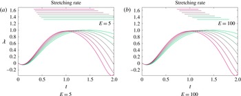
The instantaneous stretching rate (3.10) for the Duffing flow at different
 $E$
values, with the range over which a particular coloured trajectory is within the HN indicated by the lines at the top.

We first establish as before that an increase in stretching occurs when trajectories enter the HN. We choose many initial trajectory pairs near
 $(-1,1)$
, fairly close to the stable manifold. The evolution of the instantaneous stretching rate (3.10) is shown in figure 6. The upper lines indicate whether the trajectory pair identified by a particular colour lies within the HN at the origin, for each of the choices (a)
 $E=5$
and (b)
 $E=100$
. As for the Taylor–Green flow, there is a clear indication of the stretching rate increasing when close to the hyperbolic point. Using
 $E$
as a cutoff for identifying when a trajectory pair is within the HN (as used in obtaining the time ranges at the top of the figures) is once again essentially equivalent to choosing a cutoff value of the instantaneous stretching rate
 $\unicode[STIX]{x1D706}$
. Notice that we have chosen
 $E$
values that are highly disparate in this instance, and yet the results are not too different.
We next examine the impact of the nature of the HNs on stretching rates. The HN here is ‘partially degenerate’ in that it does not consist of a well-defined finite neighbourhood of the hyperbolic point as shown in figure 1, but rather is unbounded in the
 $x_{2}$
-direction. (We will define a ‘degenerate HN’ in the next section.) The asymmetry of this situation has a strong impact on the stretching rates. Consider the two initial locations
 $\unicode[STIX]{x1D6FC}$
and
 $\unicode[STIX]{x1D6FD}$
, chosen symmetrically on the two sides of the stable manifold as shown in figure 5. If taking
 $E=40$
, the forward trajectory
 $\unicode[STIX]{x1D6F7}_{\unicode[STIX]{x1D6FC}}$
through
 $\unicode[STIX]{x1D6FC}$
goes through a significant portion of the HN, but the trajectory
 $\unicode[STIX]{x1D6F7}_{\unicode[STIX]{x1D6FD}}$
through
 $\unicode[STIX]{x1D6FD}$
spends much less time within the HN. Thus, we would expect a pair of trajectories that are close to
 $\unicode[STIX]{x1D6F7}_{\unicode[STIX]{x1D6FC}}$
to have larger stretching rates than a pair close to
 $\unicode[STIX]{x1D6F7}_{\unicode[STIX]{x1D6FD}}$
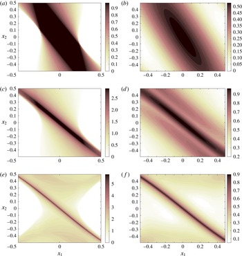
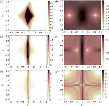
, a fact that would not be obvious without the notion of HNs. We investigate this further in figure 7. (a,c,e) Display the residence times within the HN, where we have chosen
 $E=20$
, while (b,d,f) are the forward FTLE field. We have examined the flow from the initial time
 $t=0$
to times
 $t=1$
(a,b),
 $t=3$
(c,d) and
 $t=6$
(e,f). Firstly, we note the strong correlation between the residence times and the forward FTLE fields, providing evidence that the accumulated stretching (as captured by the FTLE field) has an intimate link to how much time was spent in the HN. The longer the time spent within the HN, the longer the impact of the exponential stretching.
The residence times in the HN with
 $E=20$
(a,c,e), compared with the FTLE field (b,d,f) for the Duffing equation computed over different times from
 $t=0$
to
 $t=1$
(a,b), to
 $t=3$
(c,d) and to
 $t=6$
(e,f).

We note that there is also a fundamental difference in computing the residence time and the FTLE. For the residence time, we choose a point, iterate it in forward time, and catalogue the time spent within the HN. For an FTLE calculation, on the other hand, behaviour of nearby points is also necessary to compute the FTLE value at one point. The residence time measure is therefore an intrinsic property of each trajectory without regard to nearby motion; the strong correlation to nearby deformations, as illustrated in figure 7, is particularly interesting. Of course, we cannot claim that the residence time is better or easier to use, since it requires knowledge of the location of the hyperbolic trajectory and its accompanying neighbourhood.
As the final time value is increased, both the residence time and the FTLE plots display a sharpening ridge that, of course, approaches the stable manifold shown in figure 5. For smaller times, this ridge is less well defined, and is moreover tilted away from the true stable manifold (for which
 $x_{2}=x_{1}\sqrt{1-x_{1}^{2}/2}$
is the true expression in the vicinity of the origin, and which is well approximated by the ridges in figure 7
e,f). The reason for this tilting is clear from the asymmetry of the HNs as shown in figure 5. The HNs are symmetric about the
 $x_{2}$
-axis, and trajectories closer to this axis spend longer times within the HNs. Thus, they accumulate more stretching; i.e.
 $\unicode[STIX]{x1D6F7}_{\unicode[STIX]{x1D6FC}}$
from figure 5 will have both larger residence times and larger stretching than
 $\unicode[STIX]{x1D6F7}_{\unicode[STIX]{x1D6FD}}$
. Therefore, both the residence time and the FTLE plots will be tilted towards the
 $x_{2}$
-axis for short times, as indicated by the numerics in figure 7. Moreover, we would expect the FTLE field at
 $\unicode[STIX]{x1D6FC}$
to be larger than at
 $\unicode[STIX]{x1D6FD}$
for this reason, and this is clearly visible in figure 7(f). There is a clear patch of very low FTLE values appearing to the lower left of the FTLE ridge near
 $(-0.4,0.4)$
, in contrast with the upper right region.
Panels (a) and (b) in figure 7 are particularly instructive in interpreting FTLE fields. If figure 7(b) were considered, we might imagine that the stable manifold is tilted closer to the
 $x_{2}$
-axis than it really is. In this case we know exactly why this is so; it is because the HN – which is of infinite extent – is tilted thus, and trajectories closer to the
 $x_{2}$
axis will experience exponential stretching more. This is true for short enough times; once trajectories leave the HN, there is no longer any contribution to exponential stretching. Thus, the nature of the HNs provides additional insight into how the finite-time value used in FTLE calculations affects the final results.
3.3 Degenerate HNs
The HNs of the Duffing system did not look like the generic bounded neighbourhood shown in figure 1, in that they were unbounded. This has an influence on the FTLEs, which are a particular realization of the accumulated effects of the stretching rate (3.10). In some cases in which FTLEs give ‘unexpected’ results, we can show that this is because the HNs do not look like figure 1. We examine two examples in this section, in which the HNs are degenerate (in a way that we will define), and identify how the degenerate nature of the HNs affect the FTLEs in particular ways. First, consider the example due to Haller (Reference Haller2011), given by
 $$\begin{eqnarray}\displaystyle \left.\begin{array}{@{}c@{}}{\dot{x}}_{1}=x_{1}\\ {\dot{x}}_{2}=-x_{2}-x_{2}^{3}.\end{array}\right\} & & \displaystyle\end{eqnarray}$$
This system has a hyperbolic stagnation point at the origin, with its stable manifold along the
 $x_{2}$
-axis and its unstable manifold along the
 $x_{1}$
-axis. Thus, the initial expectation might be that the forward-time FTLE field would reveal a ridge along the
 $x_{2}$
-axis and that the backward-time FTLE field would identify a ridge along the
 $x_{1}$
-axis. However, Haller (Reference Haller2011) shows, both numerically and analytically, that the forward-time FTLE field is constant everywhere (with no ridges), and the backward-time FTLE field has a trough (rather than a ridge) along the
 $x_{1}$
-axis. This example is offered by Haller (Reference Haller2011) to show why FTLEs can fail in identifying prominent Lagrangian structures, and here we are able to use the concept of HNs to provide insight as to why FTLEs do not work.
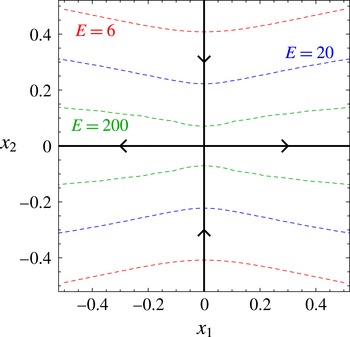
Hyperbolic neighbourhoods (boundaries shown with dashed curves) for the example of Haller (Reference Haller2011) as given in (3.19), as computed from (3.20), for
 $E=6$
(red),
 $20$
(blue) and
 $200$
(green). The stable and unstable manifolds of the origin are shown by the thick black curves.

The calculations for the HN are very similar to that for the Duffing system, and we get
 $$\begin{eqnarray}\displaystyle H=\left\{(x_{1},x_{2}):\sqrt{x_{1}^{2}+x_{2}^{2}}>E|x_{2}^{3}|\right\}. & & \displaystyle\end{eqnarray}$$
These HNs are simply a horizontal/vertical flip of the Duffing ones, and are shown in figure 8. Our first observation is that these extend infinitely in the
 $x_{1}$
-direction, thereby displaying a feature similar to figure 5. However, there is an additional characteristic: whichever
 $E$
we choose, the HN always contains the full unstable manifold. Put another way, unlike for the Taylor–Green flow (figure 2) or the Duffing equation (figure 5), each HN boundary fails to cross all manifold branches emanating from the hyperbolic trajectory. This shall be our definition for an HN to be degenerate.
Consider trajectories coming in from a positive
 $x_{2}$
value in figure 8. Whether coming in along the stable manifold or not, once they enter an HN, they will remain in it forever, because the HNs form horizontal bands around the unstable manifold, extending infinitely in
 $x_{1}$
. Thus, the trajectories will all accumulate the stretching associated with being inside an HN in the same way. The end result will be that the forward-time FTLEs will not be able to distinguish the stable manifold as a ridge. In the non-degenerate HN situation of figure 1, in contrast, it is only trajectories coming in along the stable manifold that will remain forever in the HN. The fact that all other trajectories eventually exit means that when computing forward-time FTLEs, they will eventually stop accumulating stretching, thereby resulting in a smaller FTLE value than for trajectories along the stable manifold. This explains why the forward-time FTLE field is constant and fails to identify the stable manifold as a ridge.
The backward-time FTLE failed in identifying the unstable manifold in a rather more spectacular way as shown by Haller (Reference Haller2011): the
 $x_{1}$
-axis emerges as a trough of the backward-time FTLE field rather than a ridge. That is, it has a smaller accumulation of stretching than nearby points, which appears contrary to the intuition emerging from the generic picture of figure 1. This failure is again because of the degenerate nature of the HN, but the reason is more subtle than for the forward-time FTLE. The standard expectation from a generic HN as shown in figure 1 would be that in the limit
 $E\rightarrow \infty$
, the HN would shrink towards the hyperbolic point in a smooth way, retaining connections to the stable and unstable manifolds. This is indeed illustrated for the Taylor–Green flow in figure 2, and the generic picture is that the HN is pushed outwards along the stable and unstable manifold directions. However, the situation of figure 8 is different, because of the ‘waist-like’ structure of the HNs. These pinch in exactly along the stable manifold as
 $E$
gets larger. In this degenerate situation the part of the stable manifold remaining within the HN as
 $E\rightarrow \infty$
is dramatically less than for nearby trajectories because of the inward pinching. (Indeed, it is easy to see that only a length of
 $2/\sqrt{E}$
of the stable manifold is within an HN with general
 $E$
value.) The pinching means that trajectories coming in very close to the
 $x_{1}$
-axis encounter the HN boundary having experienced far less of an excursion in the
 $x_{2}$
-direction than trajectories coming in slightly further off the
 $x_{1}$
-axis. It is these
 $x_{2}$
-excursions that contribute to stretching in backward time (since the stable manifold is in the
 $x_{2}$
-direction), and therefore trajectories along the
 $x_{1}$
-axis incur less stretching than adjacent ones. Thus, a trough rather than a ridge appears in the backward-time FTLE field.
The subtlety of this situation is further evidenced by the fact that the backward-FTLE trough is a shallow one, as shown by Haller (Reference Haller2011). In contrast, ridges identified in a non-degenerate situation like that shown in figure 1 must be sharp, since trajectories on the stable manifold remain in the HN for infinite times, in contrast with a nearby trajectory, however close. The accumulated stretching will therefore be substantially higher. To see this, we would need to ensure that the time interval over which FTLEs are computed is tuned properly, and sufficient resolution is available. Exactly how sharp is ‘sharp’ is, of course, difficult to define. In computational experiments where sharpening is observed as the ridge gets refined, as in figure 7(b,d,f), we can have confidence that this sharp ridge has an abruptly larger rate of exponential stretching than areas very near to it.
A second degenerate HN situation deserves mention. Consider the flow
 $$\begin{eqnarray}\displaystyle {\dot{x}}_{i}=\unicode[STIX]{x1D609}_{ij}x_{j} & & \displaystyle\end{eqnarray}$$
in which the
 $n\times n$
constant coefficient matrix
 $\unicode[STIX]{x1D63D}$
has one positive and one negative eigenvalue. For any trajectory of (3.21), the variational equation is then identical to (3.21) itself. In other words, a linearization is exactly correct, since there are no nonlinear terms. This reveals that all trajectories of (3.21) are hyperbolic trajectories. Moreover, the HN associated with any such hyperbolic trajectory is
 $\mathbb{R}^{n}$
in its entirety, since linearity is exactly correct everywhere. The degeneracy of this HN is because no HN boundary can be defined for an HN occupying all space. Thus, the concepts of entering and leaving HNs and of incurring exponential stretching while only being inside an HN are irrelevant. FTLE fields will therefore have no ridges (Haller Reference Haller2011; Balasuriya Reference Balasuriya2016a
).
Through the above degenerate examples and also the Duffing equation, we have shown that understanding the geometrical structure of HNs is crucial to whether the usage of FTLEs provides the intuitive information that one might expect from examining figure 1. In the Duffing equation, the HNs are only ‘partially degenerate’ in that while being unbounded, the HN boundaries did intersect all branches of the stable and unstable manifolds emanating from the hyperbolic point. In this case, subject to standard issues regarding the integration time and spatial resolution, FTLEs will manage to identify stable and unstable manifold structures, as has been done for the Duffing equation (Wiggins Reference Wiggins1992; Balasuriya Reference Balasuriya2016a ). If the HNs are genuinely degenerate, as has been argued above, FTLEs display behaviour that is at odds with the understanding provided by figure 1. Thus, HNs and their degeneracy is an additional tool for testing the capability of FTLEs (Allshouse & Peacock Reference Allshouse and Peacock2015, cf.) for identifying finite-time analogues of stable and unstable manifolds.
3.4 Oscillating Taylor–Green flow
Our next analytical example is of an unsteady, chaotic flow, initially introduced for studying transport in Rayleigh–Bénard convection by Solomon & Gollub (Reference Solomon and Gollub1988), and subsequently popular in chaotic advection studies (Babiano et al. Reference Babiano, Cartwright, Piro and Provenzale2000; Nishikawa, Toroczkai & Grebogi Reference Nishikawa, Toroczkai and Grebogi2001; Torney & Neufeld Reference Torney and Neufeld2007; Khurana, Blawzdziewicz & Ouellette Reference Khurana, Blawzdziewicz and Ouellette2011; Khurana & Ouellette Reference Khurana and Ouellette2012). It is obtained by adding a simple lateral oscillation along one of the coordinate axes to the Taylor–Green flow, so that the streamfunction is given by
 $$\begin{eqnarray}\displaystyle \unicode[STIX]{x1D713}(\boldsymbol{x},t)=\sin (x_{1}+A\sin \unicode[STIX]{x1D6FA}t)\sin x_{2} & & \displaystyle\end{eqnarray}$$
and the velocity field is
 $$\begin{eqnarray}\displaystyle \left.\begin{array}{@{}c@{}}\displaystyle {\dot{x}}_{1}=\sin (x_{1}+A\sin \unicode[STIX]{x1D6FA}t)\cos x_{2}\\ \displaystyle {\dot{x}}_{2}=-\!\cos (x_{1}+A\sin \unicode[STIX]{x1D6FA}t)\sin x_{2}.\end{array}\right\} & & \displaystyle\end{eqnarray}$$
When
 $A=0$
, this oscillating flow reduces to the steady Taylor–Green case, although, for convenience here, shifted such that the origin is a hyperbolic point. This has an unstable manifold in the
 $x_{1}$
-direction and a stable manifold in the
 $x_{2}$
-direction. For small
 $A$
, there remains a hyperbolic trajectory near the origin, although now it moves with time. Its location can be determined using Theorem 2.10 of Balasuriya (Reference Balasuriya2011) to be
 $$\begin{eqnarray}\displaystyle \bar{\boldsymbol{x}}(t)=\left(\begin{array}{@{}c@{}}\displaystyle \frac{-A[\unicode[STIX]{x1D6FA}\cos \unicode[STIX]{x1D6FA}t+\sin \unicode[STIX]{x1D6FA}t]}{1+\unicode[STIX]{x1D6FA}^{2}}\\ 0\end{array}\right)+O(A^{2})=\left(\begin{array}{@{}c@{}}\bar{x}_{1}(t)\\ 0\end{array}\right)+O(A^{2}). & & \displaystyle\end{eqnarray}$$
The velocity gradient for this flow is given by
 $$\begin{eqnarray}\displaystyle \unicode[STIX]{x1D735}\boldsymbol{u}=\left(\begin{array}{@{}cc@{}}\cos (x_{1}+A\sin \unicode[STIX]{x1D6FA}t)\cos x_{2} & -\!\sin (x_{1}+A\sin \unicode[STIX]{x1D6FA}t)\sin x_{2}\\ \sin (x_{1}+A\sin \unicode[STIX]{x1D6FA}t)\sin x_{2} & -\!\cos (x_{1}+A\sin \unicode[STIX]{x1D6FA}t)\cos x_{2}\end{array}\right), & & \displaystyle\end{eqnarray}$$
which when evaluated at
 $\bar{\boldsymbol{x}}$
becomes
 $$\begin{eqnarray}\displaystyle \unicode[STIX]{x1D735}\boldsymbol{u}(\bar{\boldsymbol{x}}(t),t)=\left(\begin{array}{@{}cc@{}}\cos (\bar{x}_{1}(t)+A\sin \unicode[STIX]{x1D6FA}t) & 0\\ 0 & -\!\cos (\bar{x}_{1}(t)+A\sin \unicode[STIX]{x1D6FA}t)\end{array}\right) & & \displaystyle\end{eqnarray}$$
so that
 $$\begin{eqnarray}\displaystyle y_{j}\frac{\unicode[STIX]{x2202}}{\unicode[STIX]{x2202}x_{j}}u_{i}(\bar{\boldsymbol{x}}(t),t)=\cos (\bar{x}_{1}(t)+A\sin \unicode[STIX]{x1D6FA}t)\left(\begin{array}{@{}c@{}}y_{1}\\ -y_{2}\end{array}\right). & & \displaystyle\end{eqnarray}$$
The velocity difference between
 $\bar{\boldsymbol{x}}(t)+\boldsymbol{y}$
and
 $\bar{\boldsymbol{x}}(t)$
is given by
 $$\begin{eqnarray}\displaystyle \boldsymbol{u}(\bar{\boldsymbol{x}}(t)+\boldsymbol{y},t)-\boldsymbol{u}(\bar{\boldsymbol{x}}(t),t) & = & \displaystyle \left(\begin{array}{@{}c@{}}\sin (\bar{x}_{1}(t)+y_{1}+A\sin \unicode[STIX]{x1D6FA}t)\cos y_{2}\\ -\!\cos (\bar{x}_{1}(t)+y_{1}+A\sin \unicode[STIX]{x1D6FA}t)\sin y_{2}\end{array}\right)\nonumber\\ \displaystyle & & \displaystyle -\!\left(\begin{array}{@{}c@{}}\sin (\bar{x}_{1}(t)+A\sin \unicode[STIX]{x1D6FA}t)\\ 0\end{array}\right).\end{eqnarray}$$
Inserting these quantities into (2.12) and using various trigonometric identities,
 $H(t)$
can then be defined as the set of points
 $(\bar{x}_{1}(t)+y_{1},y_{2})$
satisfying
 $$\begin{eqnarray}\displaystyle & & \displaystyle \cos ^{2}(\bar{x}_{1}(t)+A\sin \unicode[STIX]{x1D6FA}t)(y_{1}^{2}+y_{2}^{2})>E^{2}\left\{\left[\cos (\bar{x}_{1}(t)+A\sin \unicode[STIX]{x1D6FA}t)(y_{2}-\cos y_{1}\sin y_{2})\right.\right.\nonumber\\ \displaystyle & & \displaystyle \quad +\,\left.\sin (\bar{x}_{1}(t)+A\sin \unicode[STIX]{x1D6FA}t)\sin y_{1}\sin y_{2}\right]^{2}+\left[\sin (\bar{x}_{1}(t)+A\sin \unicode[STIX]{x1D6FA}t)(\cos y_{1}\cos y_{2}-1)\right.\nonumber\\ \displaystyle & & \displaystyle \quad +\,\left.\left.\cos (\bar{x}_{1}(t)+A\sin \unicode[STIX]{x1D6FA}t)(\sin y_{1}\cos y_{2}-y_{1})\right]^{2}\right\}.\end{eqnarray}$$
Hyperbolic neighbourhoods for the oscillating Taylor–Green flow, for parameters
 $\unicode[STIX]{x1D6FA}=2\unicode[STIX]{x03C0}$
, and
 $A=0.3$
, with the locations of the corresponding hyperbolic trajectory shown by the interior dots. Neighbourhoods are calculated (a) using a fixed
 $E=30$
at different times (
 $t=0$
(red),
 $t=0.15$
(blue) and
 $t=0.8$
(green)); and (b) at a fixed
 $t=0$
but with different values of
 $E$
(
 $E=10$
(red),
 $E=50$
(blue) and
 $E=200$
(green)).

Figure 9(a) shows the HNs as calculated from (3.29) for three different times. Notice that in this unsteady situation, the HN is not symmetric with respect to the location of the hyperbolic trajectory, unlike in the steady cases discussed above. As the hyperbolic trajectory moves back and forth, it drags the neighbourhood in which exponential attraction/repulsion reigns back and forth with it, but because it is moving in the
 $x_{1}$
-direction, this region is not symmetric with respect to
 $x_{1}$
. Also, the HN appears to move much more significantly than does the hyperbolic trajectory to which it is pinned. In contrast, there is symmetry with respect to the
 $x_{2}$
-direction because there is no hyperbolic trajectory movement in that direction. Therefore, the concept of the HN depends strongly on the Lagrangian nature of the hyperbolic trajectory, but at each instant in time identifies regions that are subject to exponential stretching or contraction as a result of this trajectory. The effect of varying
 $E$
– which identifies the relative importance of linear effects over nonlinear ones in the neighbourhood – is shown in figure 9(b). As
 $E$
gets very large, the neighbourhoods get smaller, but retain their basic structure. Importantly, they are significant patches even when the neighbourhood is defined by the linear terms being
 $200$
times greater than the nonlinear ones. Thus, exponential stretching operates over much more than an infinitesimal region near the hyperbolic trajectory. The asymmetry with respect to the hyperbolic trajectory becomes more pronounced at larger
 $E$
, highlighting the fact that its instantaneous region of influence cannot be naively assumed to be symmetric (as the conceptual figure 1 might suggest), but rather depends strongly on the Lagrangian motion of the hyperbolic trajectory. Adjacent particles entering a hyperbolic neighbourhood will experience an exponential boost to their separation while within it.
The HNs and hyperbolic trajectory locations (blue) of the oscillating Taylor–Green flow (3.23) near the origin at two different times, using
 $A=0.2$
,
 $\unicode[STIX]{x1D6FA}=2\unicode[STIX]{x03C0}$
and
 $E=50$
, with the accompanying stable (dashed green) and unstable (dashed red) manifolds also shown.

In figure 10, the relationship between the HN and the stable (green) and unstable (red) manifolds is pictured. It is easy to see that the unstable manifold of the hyperbolic point remains on the line
 $x_{2}=0$
even for
 $A\neq 0$
, since
 $x_{2}=0$
is invariant for the unsteady flow (3.23). The time-varying stable manifold is more difficult to determine. We use Theorem 2.7 from Balasuriya (Reference Balasuriya2011) to find its expression correct to
 $O(A)$
at each time
 $t$
, and display this as the dashed green curve. It is indeed possible to prove using Theorem 2.2 of Balasuriya (Reference Balasuriya2016b
) that, to
 $O(A)$
, the stable manifold continues to point vertically upwards from the hyperbolic trajectory, but when progressing away from the hyperbolic point it has a time-varying curvature. Figure 10 indicates that the HNs have no degeneracy, and so stretching accumulation will occur in the generic way. We note that there is a slight discrepancy between where the stable manifold intersects the HN and where the HN ‘sticks out’. This is because we are comparing a Lagrangian entity (the stable manifold) with an instantaneous entity (the HN) that impacts the Lagrangian motion. The instantaneous HN is continually trying to adjust itself to keep us with the time variation, and there must therefore be an effective time lag.
The stretching measure (3.10) computed for the oscillating Taylor–Green flow (3.23) with
 $A=0.2$
and
 $\unicode[STIX]{x1D6FA}=2\unicode[STIX]{x03C0}$
, for pairs of trajectories seeded near
 $(0,0.8)$
. The corresponding time in which a trajectory is inside an HN (defined according to different choices of
 $E$
as shown in each panel) is indicated by the identically coloured line towards the top of each figure.

Next, we numerically verify that trajectories experience an exponential boost when entering an HN. We use the stretching measure introduced in (3.10), and seed pairs of trajectories near
 $(0,0.8)$
, close to the stable manifold of the origin. Figure 11 shows the stretching, with each pair of trajectories having been assigned a particular colour. The domain in which the pair is deemed to be within the HN is shown by the straight lines at the top of the figures. We show the computations for four different values of
 $E$
. The stretching is clearly larger when within an HN. The fact that the HNs are oscillating with time here, unlike in the steady Taylor–Green situation, means that there are instances when trajectories leave an HN to be back inside soon afterwards, which is shown by the interrupted nature of the time-domain lines at the top of figure 11. As expected, the stretching is larger when inside an HN, and its increase when entering and decrease when leaving an HN is clearly visible.
In figure 12, we present the relationship between
 $E$
and an optimum threshold
 $\unicode[STIX]{x1D706}_{o}$
as defined in § 3.1. Figure 12(a), with
 $\unicode[STIX]{x1D706}_{o}=0.868$
, is to be compared with figure 11(b), with
 $E=20$
. The time ranges at the top of the figures obtained using these values are almost identical. The computation of the optimum
 $\unicode[STIX]{x1D706}_{o}$
for each
 $E$
value, shown in figure 12(b), in all cases is associated with an error (3.13) of approximately
 $10^{-4}$
, indicating that excellent optimality is obtained. Once again, the threshold
 $\unicode[STIX]{x1D706}_{o}$
appears to approach a constant value, and for
 $E\gtrsim 20$
, approximately 90 % of this stretching rate is achieved.
(a) The stretching rates of figure 11(b), but with the range over which
 $\unicode[STIX]{x1D706}$
is larger than a threshold value
 $\unicode[STIX]{x1D706}_{o}$
indicated by the lines at the top of the figure. (b)
 $\unicode[STIX]{x1D706}_{o}$
values as functions of
 $E$
plotted on logarithmic axes for the oscillating Taylor–Green flow, chosen by minimizing (3.13), with identical parameter values as for figure 11 being used.

The residence times in the HN with
 $E=10$
(a,c,e), compared with the FTLE field (b,d,f) for the oscillating Taylor–Green flow with
 $A=0.2$
and
 $\unicode[STIX]{x1D6FA}=2\unicode[STIX]{x03C0}$
, computed over different times from
 $t=0$
to
 $t=1$
(a,b), to
 $t=3$
(c,d) and to
 $t=7$
(e,f).

To verify that the accumulated stretching, measured via forward-time FTLEs, is related to the residence time within the HNs, we provide figure 13. The choice
 $E=10$
has been made for the HN located near the origin at time
 $0$
, and in this non-degenerate HN situation, we find that the accumulated stretching is well correlated to the residence time within the HN. Specifically, we note the qualitative similarity between the residence time and FTLE plots (how far the ridges extend, the region in which they are more peaked, where they get fatter, etc.). The horizontal ridge appearing in figure 13(f) occurs because of the stable manifold connected to the hyperbolic trajectories located near
 $(\pm \unicode[STIX]{x03C0},0)$
, which is also responsible for the larger off-ridge FTLE values appearing alongside it. The time of integration is such that particles in the chosen domain approach
 $(\pm \unicode[STIX]{x03C0},0)$
in this case, in contrast to shorter times of integration (though a hint of this issue appears in (d)). These features in (f) are not picked up in (e) because only the HN near
 $(0,0)$
has been used. The fact that this flow is genuinely unsteady has not impeded the residence time in an HN as being an excellent proxy for accumulated stretching.
4 Experimental test
Analytical examples are very useful for developing intuition about what HNs mean in situations where we know a great deal about the underlying dynamical system. The main purpose of these ideas, though, is their application in real experimental or observational data. Thus, it is important to show that the entities we define are actually computable in such a system. To that end, we here demonstrate the calculation of HNs using data from a turbulent quasi-two-dimensional laboratory flow. The insights we obtained from the analytical examples will be useful in this computation.
4.1 Apparatus and data acquisition
To generate nearly two-dimensional flow in the laboratory, we used an electromagnetically driven thin-layer flow cell we have described in detail elsewhere (Kelley & Ouellette Reference Kelley and Ouellette2011a
; Liao & Ouellette Reference Liao and Ouellette2013). The working fluid is contained in a cell of lateral dimension
 $86\times 86$
cm
 $^{2}$
, supported by a glass substrate coated in a hydrophobic wax. The fluid itself is a thin layer (roughly 5 mm deep) of an electrolyte (16 % NaCl by mass in deionized water), and so conducts electricity. We use a pair of copper bar electrodes mounted at opposite ends of the flow cell to drive d.c. electric currents of up to a few amperes through the fluid. By itself, the current does not generate flow. Underneath the glass substrate, however, lies a square grid of permanent disc magnets with their dipoles pointed vertically; the combination of the lateral current density and the vertical magnetic field applies a Lorentz body force to the fluid, which in turns generates flow. And aside from weak fringing fields from the magnets, this force lies in the plane, and so drives the fluid in a nearly two-dimensional way. The magnets themselves measure 12.7 mm in diameter, and are placed with a centre-to-centre spacing of 25.4 mm. For the experiments analysed here, they were arranged in a checkerboard fashion with the north and south poles alternating in each direction.
To measure the flow field, we use particle tracking velocimetry (PTV). We seed the fluid with small (
 $51~\unicode[STIX]{x03BC}\text{m}$
diameter) fluorescent polystyrene microspheres that absorb in the blue and emit in the green. Because these particles are lighter than the electrolyte (with a specific gravity of 1.05), they float to its surface. On the surface, though, they would experience a long-range attractive force due to surface tension. Thus, to remove this effect, we float a second layer, also 5 mm deep, of fresh water on top of the electrolyte. This miscible interface has no bulk surface tension, and so removes the particle–particle attraction, thereby rendering them faithful flow tracers (Ouellette, O’Malley & Gollub Reference Ouellette, O’Malley and Gollub2008). We illuminate the particles with blue LEDs and record their motion at a rate of 60 frames per second with an IDT MotionPro M5 camera fitted with a Schneider APO-Xenoplan lens. The camera has a resolution of
 $2320\times 1728$
pixels, with which we image the central
 $31.7\times 23.6$
cm
 $^{2}$
of the experiment (approximately
 $12\times 9$
magnet spacings). For the data we show here, the Reynolds number based on the in-plane velocity and the spacing between the magnets is
 $\text{Re}=185$
, high enough to make the flow weakly turbulent (so that it shows a net inverse energy flux from small to large scales (Kelley & Ouellette Reference Kelley and Ouellette2011b
), as is expected in two-dimensional turbulence) but not so large as to generate significant three-dimensional motion (Kelley & Ouellette Reference Kelley and Ouellette2011a
).
Images from the camera are processed to generate particle trajectories using a multiframe, predictive Lagrangian particle tracking algorithm (Ouellette, Xu & Bodenschatz Reference Ouellette, Xu and Bodenschatz2006). Accurate particle velocities are then obtained by convolving the trajectories with a differentiating and smoothing kernel (Mordant, Crawford & Bodenschatz Reference Mordant, Crawford and Bodenschatz2004). Since we track roughly 35 000 particles per frame, the instantaneous velocity measurements are spatially dense enough that we can interpolate between them to create highly resolved Eulerian velocity fields. To condition these fields further and ensure that they are as two-dimensional as possible, we project them onto a numerically computed basis of streamfunction eigenmodes (Kelley & Ouellette Reference Kelley and Ouellette2011a ). Subsequently, to generate Lagrangian statistics, we integrate the equations of motion for fluid elements through these velocity fields using second-order Runge–Kutta integration (Ouellette et al. Reference Ouellette, O’Malley and Gollub2008) to generate ‘virtual’ trajectories with any desired initial conditions.
4.2 Extraction of hyperbolic trajectories
Finding hyperbolic trajectories in an arbitrary data set can be a challenging task. The mere definition of hyperbolic trajectories in finite-time situations is fraught with difficulties, as argued for example in Balasuriya (Reference Balasuriya2016b ). Nevertheless, there is a preponderance of methods which can be adapted to find their own definition of hyperbolic trajectories, as discussed in the Introduction. The ambiguity of exactly what a hyperbolic trajectory is (as reflected by the various ‘definitions’ in use, which lead to different identifications in general) reveals an advantage of using the idea of HNs. It seems that most methods, applied with judicious interpretation and testing to a particular time-varying velocity data set, have the potential for zeroing in on essentially the same hyperbolic trajectory. However, its exact positioning will inevitably be slightly different for the different methods. Having the concept of an HN, which locates a region as opposed to a point, mitigates this uncertainty in the knowledge of the exact location.
Most of these methods (e.g. hyperbolic LCSs, Perron–Frobenius operator methods) have absolutely no direct evaluation of exponential stretching, which is what we are after. Given that this is our specific focus, we will use the method for hyperbolic trajectory identification that is explicitly designed for exponential stretching: FTLEs (Voth et al. Reference Voth, Haller and Gollub2002; Shadden et al. Reference Shadden, Lekien and Marsden2005; Lee et al. Reference Lee, Shih, Tabeling and Ho2007; Waugh et al. Reference Waugh, Abraham and Bowen2007; Samelson Reference Samelson2013; Allshouse & Peacock Reference Allshouse and Peacock2015; Balasuriya Reference Balasuriya2015a ; Huntley et al. Reference Huntley, Lipphardt, Jacobs and Kirwan2015; Johnson & Meneveau Reference Johnson and Meneveau2015; He et al. Reference He, Pan, Feng, Gao and Wang2016) as defined in (2.8). Thus, we will seek intersections between (sharp enough) ridges of the forward- and backward-time FTLE fields to determine our hyperbolic trajectories (Voth et al. Reference Voth, Haller and Gollub2002). While this process a priori does not guarantee that the identified hyperbolic trajectory is a genuine trajectory of the flow (Haller Reference Haller2015, see also figure 7(b,d,e)), we have shown that as long as the HNs remain non-degenerate, then this process conforms to the intuitive picture of figure 1, and thus intersections of stable and unstable manifolds are expected to be obtained with increasing accuracy. Checking that HNs are non-degenerate can therefore be thought of as a test for validating that FTLE ridges do indeed provide the ‘correct’ understanding of how the exponential behaviour affects fluid elements. We will a posteriori check whether the non-degeneracy property is satisfied.
In figure 14, we show the forward-time FTLE field for fixed
 $t_{0}$
and
 $T$
for our experimental flow. The field tends to organize itself into a pattern of sharp ridges. These ridges, which identify the regions of the flow field that experience the strongest stretching in the time range from
 $t_{0}$
to
 $t_{0}+T$
, mark the analogues of stable (when
 $T>0$
) and unstable (when
 $T<0$
; that is, in backwards time) manifolds. The intersections of these forward-time and backward-time ridges are then likely to mark the instantaneous positions of hyperbolic trajectories. Intersections may also be heteroclinic trajectories, but these secondary intersections can be made to be unusual in practice by investigating the behaviour of ridges as
 $T$
decreases, and verifying that FTLE ridges shorten towards the hyperbolic trajectory.
A forward-time FTLE field (blue) computed from the experimental data for a region measuring approximately
 $12\times 9$
magnet spacings. Ridges of this field, shown in green, were extracted using the procedure described in the text. The red points are the result of applying the dynamical sharpening scheme.

To extract the line-like ridges from this field data, so as to identify their forward- and backward-time intersections, we use an algorithm based on the techniques described by Senatore & Ross (Reference Senatore and Ross2011). Points that lie on or near the ridges (ridge points), shown in green in figure 14, are initially found by calculating the Hessian of the FTLE field, and identifying regions where the minimum eigenvalue, and the dot product of the corresponding eigenvector with the gradient of the FTLE field, lie within relevant tolerances. A dynamical sharpening scheme is then used to integrate the ridge points along streamlines of the field, towards the crest of the nearest ridge. Integration is stopped when the required termination condition, derived from Mathur et al. (Reference Mathur, Haller, Peacock, Ruppert-Felsot and Swinney2007), is reached; this process results in a set of points that identify the ridges. Shown in red in figure 14, these are the FTLE analogues to the unstable manifolds, and each curve must go across a hyperbolic trajectory location, as yet unknown. A similar calculation (not shown), enables the extraction of the backward-time FTLE ridges at this same instance in time. Finally, once the ridges are found in forward and backward time, it is straightforward to identify their intersection points. We treat these points as the instantaneous locations of hyperbolic trajectories.
4.3 Results
Several hyperbolic neighbourhoods superimposed on the stretching field (that is, the field of Cauchy–Green eigenvalues) from one snapshot of experimental data. Blue colours show the forward-time stretching (that is, the stable manifolds), and red colours show the backward-time stretching (that is, the unstable manifolds). The instantaneous locations of some hyperbolic trajectories are shown with black dots, and the corresponding hyperbolic neighbourhoods (calculated using
 $E=2$
) are shown with black contours. The black scale bar shows the spacing between magnets, and the Cauchy–Green tensor was computed over a time
 $T$
of approximately the correlation time of the velocity field.

Once hyperbolic trajectories have been identified, we can apply (2.12) to determine the hyperbolic neighbourhood
 $H(t)$
associated with each one at each time instant. An example is shown in figure 15, where we have used the same time instant as shown in figure 14 and have shown all the hyperbolic trajectories identified by our algorithm (which may only be a subset of the true ensemble of hyperbolic trajectories present). The instantaneous hyperbolic neighbourhoods for
 $E=2$
are shown by the black contours; the resolution of the velocity field is not sufficient to resolve HNs computed for significantly larger values of
 $E$
consistently well. Unlike in the analytical examples discussed in § 3, the HNs here are much more irregularly shaped, primarily because the flow field itself is spatially disordered. Even so, they are clearly non-degenerate, and share many features with the simple analytical examples. The HNs tend to be elongated along the stable and unstable manifolds associated with each hyperbolic trajectory, although they also extend a finite distance in other directions. It is also interesting to note that the areas of the various neighbourhoods are not at all the same; instead, some of the hyperbolic trajectories have an influence over a much larger region of space than others. This observation has significant ramifications. It is certainly reasonable to think that not every hyperbolic trajectory (along with its associated manifolds) should play an equal role in the flow dynamics; it is possible that the area of the associated hyperbolic neighbourhood may provide a way to quantify just how important a given hyperbolic trajectory is. If
 $E$
were changed uniformly across the domain, the relative sizes of the regions of influence remains unaffected. Thus, the determination of which hyperbolic trajectories are more influential over their surroundings can be made by simply choosing any reasonable
 $E$
, for example
 $E=2$
in figure 15.
There are regions in which HNs overlap, as in the top left of figure 15. Trajectories in such regions experience instantaneous stretching in the unstable manifold directions associated with each HN to which they belong. The total stretching will be a superposition of all of the directional stretchings associated with each HN the trajectory is in.
As time evolves, the HNs in this flow evolve as well, moving about and changing their shape as their associated hyperbolic trajectory moves. As they are not material areas, their size is not conserved, and they may grow or shrink with time. Far from being a failing of our technique, this shrinking contains useful information: once a hyperbolic trajectory ceases to be hyperbolic, we would expect its zone of influence to be small. This is reflected in the definition of HNs, as given in (2.12). If the linear terms vanish in comparison with the nonlinear term
 $u_{i}(\bar{\boldsymbol{x}}(t)+\boldsymbol{y},t)-u_{i}(\bar{\boldsymbol{x}}(t),t)$
, then the definition of the HN amounts to finding regions satisfying
 $0>E$
where
 $E\geqslant 1$
. That is, the HN disappears.
Finally, we examine the influence of the HNs on the stretching, as we did for our analytical examples in § 3. The situation here is, however, somewhat different, both for practical and physical reasons. Unlike in our examples, the HNs in this flow exist only for finite times and move about irregularly; thus, it is difficult to seed pairs of Lagrangian points that we know will eventually both enter an HN. Additionally, pair separation behaves differently in turbulent flows like this one and in chaotic flows like our analytical examples: trajectories separate according to a power law rather than exponentially (Sawford Reference Sawford2001; Bourgoin et al. Reference Bourgoin, Ouellette, Xu, Berg and Bodenschatz2006). In two-dimensional turbulence, however, there is expected to be a transient exponential range for initially nearby particle pairs as long as their separation remains in the range of scales in which the enstrophy cascade operates (Rivera & Ecke Reference Rivera and Ecke2005). Thus, applying (3.10) is still reasonable for initially close pairs.
We therefore computed the mean stretching rate
 $\unicode[STIX]{x1D706}$
, as defined in (3.10), averaged over both an ensemble of Lagrangian pairs initially in the HNs shown in figure 15 (computed with
 $E=2$
) and an ensemble seeded uniformly in the flow domain. Data for these two cases are shown in figure 16. The pairs used for this computation were initially separated by 2 % of the magnet spacing
 $L_{m}$
, and times are normalized by the eddy turnover time
 $T_{L}$
of eddies at the magnet scale, computed as
 $T_{L}=L_{m}/U$
, where
 $U$
is the root-mean-square velocity. Unlike the cases shown in figures 3, 6 and 11, we do not pinpoint when individual pairs enter or leave HNs in figure 16. It is clear, however, that the pairs that start in HNs do indeed experience enhanced stretching relative to a typical pair placed arbitrarily in the flow domain. Thus, even in this complex, highly unsteady flow, HNs still play a demonstrable role in boosting the Lagrangian stretching experienced by the fluid.
The mean stretching rate
 $\unicode[STIX]{x1D706}$
in the experimental flow, averaged over all the HNs shown in figure 15, as described in the text. Times are normalized by the large eddy turnover time
 $T_{L}$
. The solid, red curve shows the stretching rate for pairs initially in the HNs, while the dashed, black line shows the stretching rate for pairs seeded uniformly in the domain.

5 Discussion and conclusions
We have described here a new method for estimating the instantaneous zone of influence of a hyperbolic trajectory in arbitrary, unsteady flow by comparing the spatial structure of the velocity field to the linearized estimate around the hyperbolic trajectory. By directly analysing the linearized velocity, we have avoided ambiguities in attempting to define when a finite-time function exhibits exponential decay. We have established strong connections with FTLEs, and shown how the geometrical structure of this zone of influence can affect conclusions that can be reached through examining FTLE fields. We have verified our claim that fluid elements entering these zones of influence exhibit exponential stretching, which diminishes as they leave the zone. Thus, these zones can be thought of as travelling regions that impart anomalously large stretching on fluid elements entering them.
The essential assumption underlying this technique is the notion that if a hyperbolic trajectory (or indeed any kind of coherent structure) is to be important in a given region of the flow field, then its characteristics should be dominant to leading order in that region. In addition to being reasonable, we also note that this assumption makes our proposed technique very flexible. Here, we have defined hyperbolic neighbourhoods, in that we are characterizing the zone of influence of hyperbolic trajectories; nothing stops us, however, from extending our method to defining, e.g. elliptic or parabolic neighbourhoods, as long as the underlying point-like elliptic or parabolic structure is known. We thus anticipate that the ideas presented here may find wider application than just searching for hyperbolic structures, just as the ideas behind the original hyperbolic LCSs were later extended to include elliptic and parabolic structures (Haller Reference Haller2015).
That being said, there is still room for refinement in the ideas we have presented. As has been argued compellingly, if coherent transport is the goal, then structures that evolve in a Lagrangian sense with the flow are most worthy of investigation. While hyperbolic trajectories are Lagrangian, the hyperbolic neighbourhoods we have defined do not follow the flow. That is, particles within
 $H(t)$
at some time do not always remain within
 $H(t)$
as
 $t$
evolves. This occurs because
 $H(t)$
is defined as a moving region of influence, rather than a moving group of particles. Its defining characteristic is that while within
 $H(t)$
, fluid elements will experience instantaneous exponential stretching, as we have demonstrated through, for example, figures 3, 6 and 11. Residence time within
 $H(t)$
is also directly correlated to the stretching incurred over a given time period, as we have shown in figures 7 and 13. But unlike e.g. the Okubo–Weiss and associated criteria, the hyperbolic neighbourhoods are also not fully Eulerian, since they are pinned to the (Lagrangian) hyperbolic trajectory. In future work, we plan to explore ways of extending the Lagrangian character of the core hyperbolic trajectory to its corresponding neighbourhood by, for example, looking for advected sets that remain in instantaneous hyperbolic neighbourhood for long times.
A second productive path forward we can identify is to understand more deeply the role of the coefficient
 $E$
. We have in figures 4 and 12 shown that
 $E$
is linked to choosing a stretching threshold, i.e. how close to the stretching rate experienced at the hyperbolic point the stretching rate must be to be considered in the HN. The geometrical deformation of the HNs in the shrinking limit
 $E\rightarrow \infty$
has been shown in § 3.3 to impact on FTLEs in non-trivial ways. The value of
 $E$
can also likely be connected to the spatial resolution used in any FTLE or other Lagrangian advection computation, since HNs will be ‘visible’ in such situations only for small enough
 $E$
.
Finally, hyperbolic neighbourhoods may be a useful way to describe the stretching of transported material within a flow field. For example, consider a patch of oil that is released into an unsteady velocity field. The stretching of the oil elements will be fundamentally impacted by hyperbolic neighbourhoods in the sense that whenever some oil elements enter a hyperbolic neighbourhood, they will stretch exponentially while within it. The oil patch’s stretching over some finite time interval will therefore be strongly governed by the appearance/disappearance, locations, and time variations of hyperbolic neighbourhoods, in relation to the location of oil particles. Hyperbolic neighbourhoods thus give us a new way to think of (an aspect of) mixing, which we will pursue in the future.
Acknowledgements
The authors acknowledge support through a Terman Faculty Fellowship from Stanford University (N.T.O.), a Summer Research Scholarship from the University of Adelaide (R.K.), and Future Fellowship Grant FT130100484 from the Australian Research Council (S.B.).