1 Introduction
Over the last two decades, increased attention to causal identification has led to rapid growth in the number of randomized experiments conducted in political science, economics, and sociology. Although randomization in principle allows for the straightforward estimation of average treatment effects (ATEs) through a comparison of mean outcomes in the treatment and control groups, experimenters frequently encounter situations in which outcomes are missing for some subjects. Reasons for such missing outcome data include nonresponse in posttreatment surveys (e.g., Peress Reference Peress2010; Frankel and Hillygus Reference Frankel and Hillygus2014; Si, Reiter, and Hillygus Reference Si, Reiter and Hillygus2014), gaps in administrative records (e.g., Grogger Reference Grogger2012), and residential mobility and migration (e.g., Baird, Hamory, and Miguel Reference Baird, Hamory and Miguel2008).Footnote 1 In contrast to missing covariate information, missing outcome data threaten the validity of experimental estimates because they in effect undo the random assignment to treatment and control groups. Treatment effect estimators that ignore this missingness and consider only subjects with observed outcomes will generally be biased and inconsistent.
Researchers often address the problem of missing outcome data by introducing additional assumptions. Selection models (e.g., Heckman Reference Heckman1979; Das, Newey, and Vella Reference Das, Newey and Vella2003; see also Freedman and Sekhon Reference Freedman and Sekhon2010) require either strong parametric assumptions or an instrumental variable that is related to missingness but has no direct effect on the outcome. Such assumptions are often hard to defend on empirical or theoretical grounds. Imputation (e.g., Little and Rubin Reference Little and Rubin2002) and reweighting methods (e.g., Cassel, Särndal, and Wretman Reference Cassel, Särndal, Wretman, Madow and Olkin1983) typically presuppose that missingness is ‘ignorable’ (see Kang and Schafer (Reference Kang and Schafer2007) for a review of these methods, including “doubly robust” estimators that combine imputation and reweighting). Ignorability implies that missingness does not depend on the unobserved values of the outcome variable itself after taking into account observables. However, researchers conduct randomized experiments with the goal of drawing credible causal inferences under a minimal set of assumptions and may be reluctant to impose strong assumptions about ignorable missingness.Footnote 2
We propose a different approach to missing outcome data in randomized experiments.Footnote 3 In an effort to impose fairly weak assumptions, our approach is based on the combination of the double (or two-phase) sampling design and nonparametric worst-case bounds.Footnote 4 The double sampling design, originally due to Neyman (Reference Neyman1938), was proposed as a solution to nonresponse in survey research by Hansen and Hurwitz (Reference Hansen and Hurwitz1946). Hansen and Hurwitz (Reference Hansen and Hurwitz1946) considered cases in which an inexpensive initial survey encounters nonresponse and is then followed up with an intensive and more costly effort to interview everyone in a randomly selected subsample of initial nonrespondents. Given the probability of nonresponse in the initial survey, the variances of the outcomes among initial respondents and nonrespondents, and the costs of initial and follow-up data collection together with a budget constraint, Hansen and Hurwitz (Reference Hansen and Hurwitz1946) derived the optimal number of subjects in the initial and follow-up samples. Subsequent work has refined and extended Hansen and Hurwitz’s (Reference Hansen and Hurwitz1946) approach but maintained their assumption of no missingness among follow-up subjects (Ericson Reference Ericson1967; Kaufman and King Reference Kaufman and King1973; see also Lohr Reference Lohr2010 for a textbook discussion).
We relax this restrictive assumption to allow for missingness in both the initial sample and the follow-up sample. However, under our approach, the ATE is no longer point-identified. Nonetheless, as we show below, fundamental uncertainty about the ATE can be reduced by calculating worst-case bounds for missing outcomes in the follow-up sample. Such worst-case bounds have a long history in statistics, going back at least to Birnbaum and Sirken (Reference Birnbaum and Sirken1950a,Reference Birnbaum and Sirkenb) and Cochran, Mosteller, and Tukey (Reference Cochran, Mosteller and Tukey1954). Manski (Reference Manski1990, Reference Manski1995) has popularized their use in economics. Recent econometric work on partial identification, that is, models where only bounds on parameters of interest are identified, includes Horowitz and Manski (Reference Horowitz and Manski1998, Reference Horowitz and Manski2000), Manski (Reference Manski2007), and Lee (Reference Lee2010). Tamer (Reference Tamer2010) provides a review of this literature. Mebane and Poast (Reference Mebane and Poast2013) and Keele and Minozzi (Reference Keele and Minozzi2013) are recent contributions to the literature in political science.
Researchers have rarely drawn the connection between double sampling and worst-case bounds. In his classic textbook on survey sampling, Cochran (Reference Cochran1977) discussed both double sampling designs and worst-case bounds as techniques for dealing with survey nonresponse but did not mention the possibility of combining these two approaches. We are aware of only two works that explicitly discuss the use of double sampling in combination with bounds. The first work is DiNardo, McCrary, and Sanbonmatsu’s (Reference DiNardo, McCrary and Sanbonmatsu2006) unpublished analysis of the Moving to Opportunity field experiment, which does not consider estimation, inference, or design implications for double sampling with worst-case bounds. The second work is the textbook by Gerber and Green (Reference Gerber and Green2012, ch. 7), which presents an intuitive discussion of how double sampling and worst-case bounds may be combined to produce a narrower identification region. Gerber and Green (Reference Gerber and Green2012) presents a description of this design and illustrates with empirical examples how the estimator may substantially improve upon worst-case bounds. However, Gerber and Green (Reference Gerber and Green2012) does not present a formal derivation of the estimator. It also does not provide analytic expressions for the sampling variance of the estimator or confidence intervals and does not discuss methods for covariate adjustment in this setting.
In the next section, we show how double sampling combined with worst-case bounds partially identifies the ATE from experimental data. The double sampling approach shrinks the width of the worst-case bounds, reducing fundamental uncertainty about the ATE. Our paper thus contributes to the literature on partial identification. However, in contrast to much of this literature, which introduces additional assumptions to tighten worst-case bounds at the analysis stage, our approach modifies the data collection stage in order to shrink worst-case bounds on ATEs. We present an estimator for bounds on ATEs, variance estimators, confidence intervals, and an extension that allows for covariate adjustment via poststratification. We also propose a sensitivity analysis. We then explore the performance of our approach with a small simulation study before applying our method to a replication of a survey experiment (Levendusky and Malhotra Reference Levendusky and Malhotra2016). These examples illustrate how double sampling combined with worst-case bounds can reduce the uncertainty associated with the analysis of experiments with potentially nonignorable missing outcomes under fairly weak assumptions.
The approach proposed here applies directly to experiments in which the collection of subjects does not represent a random sample from a well-defined population, so that the sample ATE is the causal estimand of interest (see Imai, King, and Stuart (Reference Imai, King and Stuart2008) for a discussion of causal estimands). This would be the case, for example, in experiments conducted in convenience samples or experimental samples that are unrepresentative of the target population because of self-selection into the sample. We should note, however, that our proposed methodology is not designed to solve the problems involved in generalizing inferences from such samples to a target population.Footnote 5
2 Partial Identification and Estimation
In this section, we show how double sampling combined with worst-case bounds partially identifies the ATE.
2.1 Notation
Consider a completely randomized experiment with a binary treatment conducted in a sample of subjects possibly drawn at random from a large population.Footnote
6
Let
 $D_{i}$
denote subject
 $i$
’s treatment status, so that
 $D_{i}$
is equal to
 $1$
when subject
 $i$
is assigned to treatment and equal to
 $0$
when subject
 $i$
is assigned to control. We assume that compliance with treatment assignment is unproblematic, so that the assigned treatment is the same as the received treatment for all subjects (see Gerber, Green, Kaplan, and Kern (Reference Gerber, Green, Kaplan and Kern2010) for a discussion of noncompliance). Each subject has two potential outcomes, denoted
 $Y_{i}(d)$
for
 $d\in \{0,1\}$
, where
 $Y_{i}(0)$
indicates the outcome under control and
 $Y_{i}(1)$
the outcome under treatment.Footnote
7
We observe at most one of these two potential outcomes, depending on whether subject
 $i$
receives the treatment or the control, so that the outcome
 $Y_{i}=Y_{i}(1)D_{i}+Y_{i}(0)(1-D_{i})$
. When there is no attrition, the outcome
 $Y_{i}$
is observed for all subjects. From random assignment of
 $D_{i}$
and the definition of
 $Y_{i}$
, it follows that the ATE equals
 $\text{E}\,[Y_{i}(1)-Y_{i}(0)]=\text{E}\,[Y_{i}\mid D_{i}=1]-\text{E}\,[Y_{i}\mid D_{i}=0]$
. We can unbiasedly estimate the ATE by the sample analogue of the second expression, the difference in mean outcomes between the treatment and control groups. As noted above, depending on whether the set of experimental subjects can be considered a random sample from a well-defined population, the ATE corresponds to the sample ATE or the population ATE.
Some additional notation allows us to discuss the consequences of missing outcomes for the identification of the ATE. Let
 $R_{i}(d)$
denote whether subject
 $i$
’s outcome is observed when subject
 $i$
is assigned to treatment
 $d$
, with
 $R_{i}(d)$
equal to
 $1$
[
 $0$
] if subject
 $i$
’s outcome is observed [not observed] given treatment assignment
 $d$
. For example,
 $\{R_{i}(1)=1,R_{i}(0)=0\}$
indicates that subject
 $i$
’s outcome would be observed if subject
 $i$
were assigned to treatment but would not be observed if subject
 $i$
were assigned to control. Since
 $R_{i}(d)$
depends on treatment assignment, we observe either
 $R_{i}(0)$
or
 $R_{i}(1)$
but never both. The observed value of
 $R_{i}(d)$
can be written as
 $R_{i}=R_{i}(1)(D_{i})+R_{i}(0)(1-D_{i})$
.
 $Y_{i}$
is only observed when
 $R_{i}(d)=1$
; thus, the marginal distributions of
 $Y_{i}(1)$
and
 $Y_{i}(0)$
can only be observed conditional on
 $R_{i}(1)=1$
and
 $R_{i}(0)=1$
, respectively.
Attrition may lead to bias in a simple comparison of treatment and control means when missingness is related to potential outcomes
 $Y_{i}(0)$
and
 $Y_{i}(1)$
. To see this, note that the expected outcome in the treatment group can be written as a weighted average, as in
 $$\begin{eqnarray}\displaystyle \text{E}\,[Y_{i}\mid D_{i}=1] & = & \displaystyle \text{E}\,[R_{i}\mid D_{i}=1]\cdot \text{E}\,[Y_{i}\mid D_{i}=1,R_{i}=1]\nonumber\\ \displaystyle & & \displaystyle +\,(1-\text{E}\,[R_{i}\mid D_{i}=1])\cdot \text{E}\,[Y_{i}\mid D_{i}=1,R_{i}=0].\end{eqnarray}$$
Likewise, the expected outcome in the control group can be written as
 $$\begin{eqnarray}\displaystyle \text{E}\,[Y_{i}\mid D_{i}=0] & = & \displaystyle \text{E}\,[R_{i}\mid D_{i}=0]\cdot \text{E}\,[Y_{i}\mid D_{i}=0,R_{i}=1]\nonumber\\ \displaystyle & & \displaystyle +\,(1-\text{E}\,[R_{i}\mid D_{i}=0])\cdot \text{E}\,[Y_{i}\mid D_{i}=0,R_{i}=0].\end{eqnarray}$$
These two expressions are not point-identified since the data are not informative about
 $\text{E}\,[Y_{i}\mid D_{i}=1,R_{i}=0]$
or
 $\text{E}\,[Y_{i}\mid D_{i}=0,R_{i}=0]$
. However, suppose
 $Y_{i}(D_{i}=d)\bot \!\!\!\!\!\bot R_{i}(D_{i}=d)$
for
 $d\in \{0,1\}$
, so that missingness is independent of potential outcomes. (As usual,
 $\bot \!\!\!\!\!\bot$
denotes statistical independence.) Then the equality
 $$\begin{eqnarray}\text{E}\,[Y_{i}\mid D_{i}=d]=\text{E}\,[Y_{i}\mid D_{i}=d,R_{i}=1]=\text{E}\,[Y_{i}\mid D_{i}=d,R_{i}=0]=\text{E}\,[Y_{i}(d)]\end{eqnarray}$$
holds, in which case the ATE is point-identified and can be estimated by comparing the means of the observed outcomes in the treatment and control groups.Footnote 8
2.2 Worst-case bounds
Suppose we are unwilling to assume that missingness is independent of potential outcomes (even conditional on covariates). A fallback approach is to put worst-case bounds on the ATE. These bounds are sharp, i.e., they are the narrowest bounds possible unless additional assumptions are introduced (Manski Reference Manski2007). Assume that the support of the outcome variable is bounded, with
 $y^{L}$
denoting the lower bound and
 $y^{U}$
denoting the upper bound. It is then possible to bound the expected outcome in the treated group,
 $\text{E}\,[Y_{i}\mid D_{i}=1]$
, by assuming that the missing outcomes take the smallest possible value
 $y^{L}$
or the largest possible value
 $y^{U}$
:
 $$\begin{eqnarray}\displaystyle & & \displaystyle \text{E}\,[R_{i}\mid D_{i}=1]\cdot \text{E}\,[Y_{i}\mid D_{i}=1,R_{i}=1]+(1-\text{E}\,[R_{i}\mid D_{i}=1])\cdot y^{L}\nonumber\\ \displaystyle & & \displaystyle \quad \leqslant \text{E}\,[Y_{i}\mid D_{i}=1]=\text{E}\,[Y_{i}(1)]\nonumber\\ \displaystyle & & \displaystyle \quad \leqslant \text{E}\,[R_{i}\mid D_{i}=1]\cdot \text{E}\,[Y_{i}\mid D_{i}=1,R_{i}=1]+(1-\text{E}\,[R_{i}\mid D_{i}=1])\cdot y^{U}.\end{eqnarray}$$
Bounds for the expected outcome in the control group are formed the same way, so that
 $$\begin{eqnarray}\displaystyle & & \displaystyle \text{E}\,[R_{i}\mid D_{i}=0]\cdot \text{E}\,[Y_{i}\mid D_{i}=0,R_{i}=1]+(1-\text{E}\,[R_{i}\mid D_{i}=0])\cdot y^{L}\nonumber\\ \displaystyle & & \displaystyle \quad \leqslant \text{E}\,[Y_{i}\mid D_{i}=0]=\text{E}\,[Y_{i}(0)]\nonumber\\ \displaystyle & & \displaystyle \quad \leqslant \text{E}\,[R_{i}\mid D_{i}=0]\cdot \text{E}\,[Y_{i}\mid D_{i}=0,R_{i}=1]+(1-\text{E}\,[R_{i}\mid D_{i}=0])\cdot y^{U}.\end{eqnarray}$$
We then form the lower bound on the ATE by subtracting the upper bound on the expected outcome under control from the lower bound on the expected outcome under treatment. The upper bound on the ATE is formed by subtracting the lower bound on the expected outcome under control from the upper bound on the expected outcome under treatment:
 $$\begin{eqnarray}\displaystyle & & \displaystyle \text{E}\,[R_{i}\mid D_{i}=1]\cdot \text{E}\,[Y_{i}\mid D_{i}=1,R_{i}=1]+(1-\text{E}\,[R_{i}\mid D_{i}=1])\cdot y^{L}\nonumber\\ \displaystyle & & \displaystyle \qquad -\left[\text{E}\,[R_{i}\mid D_{i}=0]\cdot \text{E}\,[Y_{i}\mid D_{i}=0,R_{i}=1]+(1-\text{E}\,[R_{i}\mid D_{i}=0])\cdot y^{U}\right]\nonumber\\ \displaystyle & & \displaystyle \quad \leqslant \text{E}\,[Y_{i}\mid D_{i}=1]-\text{E}\,[Y_{i}\mid D_{i}=0]=\text{E}\,[Y_{i}(1)-Y_{i}(0)]\nonumber\\ \displaystyle & & \displaystyle \quad \leqslant \text{E}\,[R_{i}\mid D_{i}=1]\cdot \text{E}\,[Y_{i}\mid D_{i}=1,R_{i}=1]+(1-\text{E}\,[R_{i}\mid D_{i}=1])\cdot y^{U}\nonumber\\ \displaystyle & & \displaystyle \qquad -\left[\text{E}\,[R_{i}\mid D_{i}=0]\cdot \text{E}\,[Y_{i}\mid D_{i}=0,R_{i}=1]+(1-\text{E}\,[R_{i}\mid D_{i}=0])\cdot y^{L}\right].\end{eqnarray}$$
It is easy to show that the bounds on the expected outcomes in the control and treatment groups have widths equal to
 $y^{U}-y^{L}$
times the fractions of missing outcomes. The width of the bound on the ATE is equal to the sum of the widths of these two bounds. When the fraction of missing outcomes is appreciable, worst-case bounds on the ATE thus tend to be wide and not very informative. However, as we show in the next section of the paper, we can often dramatically reduce the width of the identification region by combining worst-case bounds with the double sampling design.
2.3 Double sampling
The basic insight behind the double sampling design is that we can eliminate or at least reduce the adverse consequences of missing outcome data by directing an intensive follow-up effort at a randomly selected subsample of subjects with initially missing outcomes.Footnote
9
Let
 $F_{i}$
denote whether subject
 $i$
is randomly assigned to the follow-up sample, with
 $F_{i}$
equal to
 $1$
[
 $0$
] if subject
 $i$
is assigned [not assigned] to the follow-up sample. Because only subjects with initially missing outcomes are assigned to the follow-up sample,
 $\Pr (F_{i}=1\mid R_{i}=1)=0$
for all
 $i$
.
The double sampling design rests on the assumption that potential outcomes are invariant across data collection rounds, so that it does not matter whether we observe outcomes in the initial sample or the follow-up sample. We call this assumption outcome stability. Importantly, note that this assumption allows for arbitrary differences between observations with initially missing and initially observed outcomes. We do not have to assume that, perhaps conditional on covariates, outcomes for the latter group can be used to impute outcomes for the former group.
Outcome stability can be violated in different ways. For example, if the mode of data collection in the initial sample is different from the mode of data collection in the follow-up sample, outcome stability does not hold if the mode of data collection itself affects outcomes. In Hansen and Hurwitz (Reference Hansen and Hurwitz1946), the implicit assumption is that how subjects with initially missing outcomes respond when interviewed in the follow-up round (face to face) is identical to how the same subjects would have responded when surveyed in the initial round (by mail). Outcome stability is also violated if the follow-up data collection offers monetary incentives to increase responsiveness and these incentives affect subjects’ responses. Finally, outcome stability fails to hold if treatment effects decay (or increase) over time and there exists an appreciable time gap between the initial outcome data collection and the follow-up data collection.
Researchers using a double sampling design to address missing outcome data in randomized experiments should explicitly discuss the plausibility of outcome stability in light of their specific application, in particular with respect to differences between data collection procedures in the initial sample and the follow-up sample and the time gap between initial and follow-up data collection.
In order to see the intuition behind double sampling under outcome stability, consider the following case. Assume for the moment, following Hansen and Hurwitz (Reference Hansen and Hurwitz1946), that follow-up data collection is entirely successful, so that we obtain outcomes for every subject in the follow-up sample. Also assume that the follow-up sample contains both treated and control subjects, which is easily assured through random sampling within strata defined by treatment assignment. Since the follow-up sample is a stratified random sample from the subgroups of control and treated subjects with initially missing outcomes,
 $\{i:D_{i}=0,R_{i}=0\}$
and
 $\{i:D_{i}=1,R_{i}=0\}$
, it is clear that the outcomes observed in the follow-up sample are sufficient to identify
 $\text{E}\,[Y_{i}\mid D_{i}=0,R_{i}=0]$
and
 $\text{E}\,[Y_{i}\mid D_{i}=1,R_{i}=0]$
when outcome stability holds. That is, when outcomes in the follow-up sample are fully observed and outcome stability holds, all terms in (1) and (2) are point-identified either from the initial sample or the follow-up sample, so that the sample analogues of (1) and (2) can be used to estimate the ATE.
2.4 Double sampling and bounds combined
To deal with situations in which we fail to observe outcomes for every subject in the follow-up sample, let
 $S_{i}(d)$
denote whether subject
 $i$
’s outcome is observed in the follow-up sample when subject
 $i$
is assigned to treatment
 $d$
, with
 $S_{i}(d)$
equal to
 $1$
[
 $0$
] if subject
 $i$
’s outcome is observed [not observed] in the follow-up sample given treatment assignment
 $d$
. For example,
 $\{S_{i}(1)=1,S_{i}(0)=0\}$
indicates that subject
 $i$
’s outcome would be observed in the follow-up sample if subject
 $i$
were assigned to treatment but would not be observed if subject
 $i$
were assigned to control. Of course,
 $S_{i}=S_{i}(1)D_{i}+S_{i}(0)(1-D_{i})$
is only observed for subjects randomly assigned to the follow-up sample, that is, subjects for which
 $F_{i}=1$
.
Recall from (1) that we can write the expected outcome in the treatment group as a weighted average and that the sampling process identifies all expectations except
 $\text{E}\,[Y_{i}\mid D_{i}=1,R_{i}=0]$
. If outcome stability holds,
 $\text{E}\,[Y_{i}\mid D_{i}=1,R_{i}=0]=\text{E}\,[Y_{i}\mid D_{i}=1,R_{i}=0,F_{i}=1]=\text{E}\,[Y_{i}\mid D_{i}=1,F_{i}=1]$
, where the first equality follows from stratified random sampling, which implies
 $Y_{i}\bot \!\!\!\!\!\bot F_{i}\mid D_{i}=1,R_{i}=0$
, and the second equality follows from the definition of
 $F_{i}$
. We can write
 $$\begin{eqnarray}\displaystyle \text{E}\,[Y_{i}\mid D_{i}=1,F_{i}=1] & = & \displaystyle \text{E}\,[S_{i}\mid D_{i}=1,F_{i}=1]\cdot \text{E}\,[Y_{i}\mid D_{i}=1,F_{i}=1,S_{i}=1]\nonumber\\ \displaystyle & & \displaystyle +\,(1-\text{E}\,[S_{i}\mid D_{i}=1,F_{i}=1])\cdot \text{E}\,[Y_{i}\mid D_{i}=1,F_{i}=1,S_{i}=0].\end{eqnarray}$$
All terms in expression (6) are point-identified with the exception of the expected outcome in the follow-up treatment group among subjects for which follow-up outcomes are missing,
 $\text{E}\,[Y_{i}\mid D_{i}=1,F_{i}=1,S_{i}=0]$
. Again, we can bound this term by substituting in
 $y^{L}$
and
 $y^{U}$
to get the lower and upper bounds, respectively:
The lower bound equals
 $$\begin{eqnarray}\displaystyle \text{E}\,[Y_{i}\mid D_{i}=1,F_{i}=1]^{L} & = & \displaystyle \text{E}\,[S_{i}\mid D_{i}=1,F_{i}=1]\cdot \text{E}\,[Y_{i}\mid D_{i}=1,F_{i}=1,S_{i}=1]\nonumber\\ \displaystyle & & \displaystyle +\,(1-\text{E}\,[S_{i}\mid D_{i}=1,F_{i}=1])\cdot y^{L}.\end{eqnarray}$$
The upper bound equals
 $$\begin{eqnarray}\displaystyle \text{E}\,[Y_{i}\mid D_{i}=1,F_{i}=1]^{U} & = & \displaystyle \text{E}\,[S_{i}\mid D_{i}=1,F_{i}=1]\cdot \text{E}\,[Y_{i}\mid D_{i}=1,F_{i}=1,S_{i}=1]\nonumber\\ \displaystyle & & \displaystyle +\,(1-\text{E}\,[S_{i}\mid D_{i}=1,F_{i}=1])\cdot y^{U}.\end{eqnarray}$$
Bounds on
 $\text{E}\,[Y_{i}\mid D_{i}=0,F_{i}=1]$
are constructed the same way, yielding
 $$\begin{eqnarray}\displaystyle \text{E}\,[Y_{i}\mid D_{i}=0,F_{i}=1]^{L} & = & \displaystyle \text{E}\,[S_{i}\mid D_{i}=0,F_{i}=1]\cdot \text{E}\,[Y_{i}\mid D_{i}=0,F_{i}=1,S_{i}=1]\nonumber\\ \displaystyle & & \displaystyle +\,(1-\text{E}\,[S_{i}\mid D_{i}=0,F_{i}=1])\cdot y^{L}\end{eqnarray}$$
and
 $$\begin{eqnarray}\displaystyle \text{E}\,[Y_{i}\mid D_{i}=0,F_{i}=1]^{U} & = & \displaystyle \text{E}\,[S_{i}\mid D_{i}=0,F_{i}=1]\cdot \text{E}\,[Y_{i}\mid D_{i}=0,F_{i}=1,S_{i}=1]\nonumber\\ \displaystyle & & \displaystyle +\,(1-\text{E}\,[S_{i}\mid D_{i}=0,F_{i}=1])\cdot y^{U}.\end{eqnarray}$$
Substituting these four bounds into (1) and (2) then yields bounds on the expected outcomes in the treatment and control groups based on the double sampling design. The lower bound for the expected outcome in the treatment group equals
 $$\begin{eqnarray}\displaystyle \text{E}\,[Y_{i}\mid D_{i}=1]^{L} & = & \displaystyle \text{E}\,[R_{i}\mid D_{i}=1]\cdot \text{E}\,[Y_{i}\mid D_{i}=1,R_{i}=1]\nonumber\\ \displaystyle & & \displaystyle +\,(1-\text{E}\,[R_{i}\mid D_{i}=1])\cdot \text{E}\,[Y_{i}\mid D_{i}=1,F_{i}=1]^{L}\nonumber\\ \displaystyle & = & \displaystyle \text{E}\,[R_{i}\mid D_{i}=1]\cdot \text{E}\,[Y_{i}\mid D_{i}=1,R_{i}=1]+(1-\text{E}\,[R_{i}\mid D_{i}=1])\nonumber\\ \displaystyle & & \displaystyle \cdot \,\big(\text{E}\,[S_{i}\mid D_{i}=1,F_{i}=1]\cdot \text{E}\,[Y_{i}\mid D_{i}=1,F_{i}=1,S_{i}=1]\nonumber\\ \displaystyle & & \displaystyle +\,(1-\text{E}\,[S_{i}\mid D_{i}=1,F_{i}=1])\cdot y^{L}\big).\end{eqnarray}$$
The upper bound equals
 $$\begin{eqnarray}\displaystyle \text{E}\,[Y_{i}\mid D_{i}=1]^{U} & = & \displaystyle \text{E}\,[R_{i}\mid D_{i}=1]\cdot \text{E}\,[Y_{i}\mid D_{i}=1,R_{i}=1]\nonumber\\ \displaystyle & & \displaystyle +\,(1-\text{E}\,[R_{i}\mid D_{i}=1])\cdot \text{E}\,[Y_{i}\mid D_{i}=1,F_{i}=1]^{U}\nonumber\\ \displaystyle & = & \displaystyle \text{E}\,[R_{i}\mid D_{i}=1]\cdot \text{E}\,[Y_{i}\mid D_{i}=1,R_{i}=1]+(1-\text{E}\,[R_{i}\mid D_{i}=1])\nonumber\\ \displaystyle & & \displaystyle \cdot \,\big(\text{E}\,[S_{i}\mid D_{i}=1,F_{i}=1]\cdot \text{E}\,[Y_{i}\mid D_{i}=1,F_{i}=1,S_{i}=1]\nonumber\\ \displaystyle & & \displaystyle +\,(1-\text{E}\,[S_{i}\mid D_{i}=1,F_{i}=1])\cdot y^{U}\big).\end{eqnarray}$$
Analogous expressions hold for the control group, yielding
 $$\begin{eqnarray}\displaystyle \text{E}\,[Y_{i}\mid D_{i}=0]^{L} & = & \displaystyle \text{E}\,[R_{i}\mid D_{i}=0]\cdot \text{E}\,[Y_{i}\mid D_{i}=0,R_{i}=1]\nonumber\\ \displaystyle & & \displaystyle +\,(1-\text{E}\,[R_{i}\mid D_{i}=0])\cdot \text{E}\,[Y_{i}\mid D_{i}=0,F_{i}=1]^{L}\nonumber\\ \displaystyle & = & \displaystyle \text{E}\,[R_{i}\mid D_{i}=0]\cdot \text{E}\,[Y_{i}\mid D_{i}=0,R_{i}=1]+(1-\text{E}\,[R_{i}\mid D_{i}=0])\nonumber\\ \displaystyle & & \displaystyle \cdot \,\big(\text{E}\,[S_{i}\mid D_{i}=0,F_{i}=1]\cdot \text{E}\,[Y_{i}\mid D_{i}=0,F_{i}=1,S_{i}=1]\nonumber\\ \displaystyle & & \displaystyle +\,(1-\text{E}\,[S_{i}\mid D_{i}=0,F_{i}=1])\cdot y^{L}\big).\end{eqnarray}$$
and
 $$\begin{eqnarray}\displaystyle \text{E}\,[Y_{i}\mid D_{i}=0]^{U} & = & \displaystyle \text{E}\,[R_{i}\mid D_{i}=0]\cdot \text{E}\,[Y_{i}\mid D_{i}=0,R_{i}=1]\nonumber\\ \displaystyle & & \displaystyle +\,(1-\text{E}\,[R_{i}\mid D_{i}=0])\cdot \text{E}\,[Y_{i}\mid D_{i}=0,F_{i}=1]^{U}\nonumber\\ \displaystyle & = & \displaystyle \text{E}\,[R_{i}\mid D_{i}=0]\cdot \text{E}\,[Y_{i}\mid D_{i}=0,R_{i}=1]+(1-\text{E}\,[R_{i}\mid D_{i}=0])\nonumber\\ \displaystyle & & \displaystyle \cdot \,\bigg(\text{E}\,[S_{i}\mid D_{i}=0,F_{i}=1]\cdot \text{E}\,[Y_{i}\mid D_{i}=0,F_{i}=1,S_{i}=1]\nonumber\\ \displaystyle & & \displaystyle +\,(1-\text{E}\,[S_{i}\mid D_{i}=0,F_{i}=1])\cdot y^{U}\bigg).\end{eqnarray}$$
The bounds on the ATE are formed as in (5). To compute the lower bound on the ATE, we subtract the upper bound on the expected outcome under control (Equation (14)) from the lower bound on the expected outcome under treatment (Equation (11)). To compute the upper bound on the ATE, we subtract the lower bound on the expected outcome under control (Equation (13)) from the upper bound on the expected outcome under treatment (Equation (12)). Formally, the bounds on the ATE are given by
 $$\begin{eqnarray}\displaystyle & & \displaystyle \text{E}\,[R_{i}\mid D_{i}=1]\cdot \text{E}\,[Y_{i}\mid D_{i}=1,R_{i}=1]+(1-\text{E}\,[R_{i}\mid D_{i}=1])\nonumber\\ \displaystyle & & \displaystyle \qquad \cdot \,\big(\text{E}\,[S_{i}\mid D_{i}=1,F_{i}=1]\cdot \text{E}\,[Y_{i}\mid D_{i}=1,F_{i}=1,S_{i}=1]\nonumber\\ \displaystyle & & \displaystyle \qquad +\,(1-\text{E}\,[S_{i}\mid D_{i}=1,F_{i}=1])\cdot y^{L}\big)\nonumber\\ \displaystyle & & \displaystyle \qquad -\left[\vphantom{y^{L}\big)}\text{E}\,[R_{i}\mid D_{i}=0]\cdot \text{E}\,[Y_{i}\mid D_{i}=0,R_{i}=1]+(1-\text{E}\,[R_{i}\mid D_{i}=0])\right.\nonumber\\ \displaystyle & & \displaystyle \qquad \cdot \,\big(\text{E}\,[S_{i}\mid D_{i}=0,F_{i}=1]\cdot \text{E}\,[Y_{i}\mid D_{i}=0,F_{i}=1,S_{i}=1]\nonumber\\ \displaystyle & & \displaystyle \qquad \left.+\,(1-\text{E}\,[S_{i}\mid D_{i}=0,F_{i}=1])\cdot y^{U}\big)\right]\nonumber\\ \displaystyle & & \displaystyle \quad \leqslant \text{E}\,[Y_{i}\mid D_{i}=1]-\text{E}\,[Y_{i}\mid D_{i}=0]=\text{E}\,[Y_{i}(1)-Y_{i}(0)]\nonumber\\ \displaystyle & & \displaystyle \quad \leqslant \text{E}\,[R_{i}\mid D_{i}=1]\cdot \text{E}\,[Y_{i}\mid D_{i}=1,R_{i}=1]+(1-\text{E}\,[R_{i}\mid D_{i}=1])\nonumber\\ \displaystyle & & \displaystyle \qquad \cdot \,\big(\text{E}\,[S_{i}\mid D_{i}=1,F_{i}=1]\cdot \text{E}\,[Y_{i}\mid D_{i}=1,F_{i}=1,S_{i}=1]\nonumber\\ \displaystyle & & \displaystyle \qquad +\,(1-\text{E}\,[S_{i}\mid D_{i}=1,F_{i}=1])\cdot y^{U}\big)\nonumber\\ \displaystyle & & \displaystyle \qquad -\left[\vphantom{y^{L}\big)}\text{E}\,[R_{i}\mid D_{i}=0]\cdot \text{E}\,[Y_{i}\mid D_{i}=0,R_{i}=1]+(1-\text{E}\,[R_{i}\mid D_{i}=0])\right.\nonumber\\ \displaystyle & & \displaystyle \qquad \cdot \,\big(\text{E}\,[S_{i}\mid D_{i}=0,F_{i}=1]\cdot \text{E}\,[Y_{i}\mid D_{i}=0,F_{i}=1,S_{i}=1]\nonumber\\ \displaystyle & & \displaystyle \qquad \left.+\,(1-\text{E}\,[S_{i}\mid D_{i}=0,F_{i}=1])\cdot y^{L}\big)\right].\end{eqnarray}$$
Let
 $\unicode[STIX]{x1D70F}$
denote the ATE, let
 $\unicode[STIX]{x1D70F}^{L}$
denote the lower bound on
 $\unicode[STIX]{x1D70F}$
, and let
 $\unicode[STIX]{x1D70F}^{U}$
denote the upper bound on
 $\unicode[STIX]{x1D70F}$
(all given in (15)), so that
 $$\begin{eqnarray}\displaystyle \unicode[STIX]{x1D70F}^{L}\leqslant \unicode[STIX]{x1D70F}\leqslant \unicode[STIX]{x1D70F}^{U}. & & \displaystyle\end{eqnarray}$$
The identification region for the ATE is denoted by
 $[\unicode[STIX]{x1D70F}^{L},\unicode[STIX]{x1D70F}^{U}]$
. If outcome stability holds, the ATE must lie in this interval, although it cannot be pinpointed any further unless we are willing to introduce additional assumptions. See Manski (Reference Manski1990, Reference Manski1995, Reference Manski2007), Zhang and Rubin (Reference Zhang and Rubin2004), and Lee (Reference Lee2010) for a discussion of the use of additional assumptions to further narrow worst-case bounds on quantities of interest and Manski and Nagin (Reference Manski and Nagin1998), Manski and Pepper (Reference Manski and Pepper2011), Mebane and Poast (Reference Mebane and Poast2013), and Keele and Minozzi (Reference Keele and Minozzi2013) for empirical examples.
2.5 Estimation and inference
Let
 $n_{(c)1}$
be the number of control subjects for whom we attempt to measure outcomes initially and let
 $p_{(c)1}$
be the proportion of control subjects for which we observe outcomes in the initial sample. From among the
 $(1-p_{(c)1})n_{(c)1}$
control subjects for which we initially fail to observe outcomes, a random follow-up sample of size
 $n_{(c)2}$
is taken, with
 $2\leqslant n_{(c)2}\leqslant (1-p_{(c)1})n_{(c)1}$
. Let
 $p_{(c)2}$
be the proportion of control subjects for which we observe outcomes in the follow-up sample. Let
 $s_{(c)1}^{2}$
denote the sample variance of the outcome variable among control subjects with observed outcomes in the initial sample. Let
 $s_{(c)2L}^{2}$
denote the sample variance of the outcome variable among control subjects in the follow-up sample with missing outcomes substituted by
 $y^{L}$
and
 $s_{(c)2U}^{2}$
the sample variance of the outcome variable among control subjects in the follow-up sample with missing outcomes substituted by
 $y^{U}$
. Finally, let
 $\bar{y}_{(c)1}$
be the sample mean among control subjects with observed outcomes in the initial sample, let
 $\bar{y}_{(c)2}$
be the sample mean among control subjects with observed outcomes in the follow-up sample, and let
 $\bar{y}_{(c)2L}$
and
 $\bar{y}_{(c)2U}$
denote the lower and upper bounds on the sample mean among control subjects in the follow-up sample after substituting
 $y^{L}$
and
 $y^{U}$
for missing outcomes. For the treatment group,
 $n_{(t)1}$
,
 $p_{(t)1}$
,
 $n_{(t)2}$
,
 $p_{(t)2}$
,
 $s_{(t)1}^{2}$
,
 $s_{(t)2L}^{2}$
,
 $s_{(t)2U}^{2}$
,
 $\bar{y}_{(t)1}$
,
 $\bar{y}_{(t)2}$
,
 $\bar{y}_{(t)2L}$
, and
 $\bar{y}_{(t)2U}$
are defined analogously.
We can use the sample analogues of the expressions in (15) to estimate lower and upper bounds on the ATE. Call these estimated lower and upper bounds
 $\widehat{\unicode[STIX]{x1D70F}}^{L}$
and
 $\widehat{\unicode[STIX]{x1D70F}}^{U}$
, respectively. From (15), we have
 $$\begin{eqnarray}\displaystyle \widehat{\unicode[STIX]{x1D70F}}^{L} & = & \displaystyle p_{(t)1}\cdot \bar{y}_{(t)1}+(1-p_{(t)1})\cdot \big(p_{(t)2}\cdot \bar{y}_{(t)2}+(1-p_{(t)2})\cdot y^{L}\big)\nonumber\\ \displaystyle & & \displaystyle -\left[p_{(c)1}\cdot \bar{y}_{(c)1}+(1-p_{(c)1})\cdot \big(p_{(c)2}\cdot \bar{y}_{(c)2}+(1-p_{(c)2})\cdot y^{U}\big)\right]\end{eqnarray}$$
and
 $$\begin{eqnarray}\displaystyle \widehat{\unicode[STIX]{x1D70F}}^{U} & = & \displaystyle p_{(t)1}\cdot \bar{y}_{(t)1}+(1-p_{(t)1})\cdot \big(p_{(t)2}\cdot \bar{y}_{(t)2}+(1-p_{(t)2})\cdot y^{U}\big)\nonumber\\ \displaystyle & & \displaystyle -\left[p_{(c)1}\cdot \bar{y}_{(c)1}+(1-p_{(c)1})\cdot \big(p_{(c)2}\cdot \bar{y}_{(c)2}+(1-p_{(c)2})\cdot y^{L}\big)\right].\end{eqnarray}$$
The asymptotic variance of the double sampling estimator is given in Glynn, Laird, and Rubin (1993, equation 2) (see also Rao Reference Rao1973 and Cochran Reference Cochran1977). Their assumptions are identical to ours; we do omit a finite-population correction factor. Applying this formula yields expressions for the variances of the lower and upper bounds on the mean outcomes in the control and treatment groups:
 $$\begin{eqnarray}\displaystyle \widehat{\unicode[STIX]{x1D70E}}_{(c)_{L}}^{2} & = & \displaystyle \frac{p_{(c)1}s_{(c)1}^{2}}{n_{(c)1}}+\frac{(1-p_{(c)1})^{2}s_{(c)2L}^{2}}{n_{(c)2}}+\frac{(1-p_{(c)1})p_{(c)1}(\bar{y}_{(c)_{2L}}-\bar{y}_{(c)1})^{2}}{n_{(c)1}},\end{eqnarray}$$
 $$\begin{eqnarray}\displaystyle \widehat{\unicode[STIX]{x1D70E}}_{(c)_{U}}^{2} & = & \displaystyle \frac{p_{(c)1}s_{(c)1}^{2}}{n_{(c)1}}+\frac{(1-p_{(c)1})^{2}s_{(c)2U}^{2}}{n_{(c)2}}+\frac{(1-p_{(c)1})p_{(c)1}(\bar{y}_{(c)_{2U}}-\bar{y}_{(c)1})^{2}}{n_{(c)1}},\end{eqnarray}$$
 $$\begin{eqnarray}\displaystyle \widehat{\unicode[STIX]{x1D70E}}_{(t)_{L}}^{2} & = & \displaystyle \frac{p_{(t)1}s_{(t)1}^{2}}{n_{(t)1}}+\frac{(1-p_{(t)1})^{2}s_{(t)2L}^{2}}{n_{(t)2}}+\frac{(1-p_{(t)1})p_{(t)1}(\bar{y}_{(t)_{2L}}-\bar{y}_{(t)1})^{2}}{n_{(t)1}},\end{eqnarray}$$
 $$\begin{eqnarray}\displaystyle \widehat{\unicode[STIX]{x1D70E}}_{(t)_{U}}^{2} & = & \displaystyle \frac{p_{(t)1}s_{(t)1}^{2}}{n_{(t)1}}+\frac{(1-p_{(t)1})^{2}s_{(t)2U}^{2}}{n_{(t)2}}+\frac{(1-p_{(t)1})p_{(t)1}(\bar{y}_{(t)_{2U}}-\bar{y}_{(t)1})^{2}}{n_{(t)1}}.\end{eqnarray}$$
Using Neyman’s estimator for the variance of the treatment effect in completely randomized experiments, except that we estimate group variances based on the double sampling estimators given in (19)–(22), the standard error of the lower bound on the ATE is equal to
 $\sqrt{\widehat{\unicode[STIX]{x1D70E}}_{(t)_{L}}^{2}+\widehat{\unicode[STIX]{x1D70E}}_{(c)_{U}}^{2}}$
and the standard error of the upper bound is equal to
 $\sqrt{\widehat{\unicode[STIX]{x1D70E}}_{(t)_{U}}^{2}+\widehat{\unicode[STIX]{x1D70E}}_{(c)_{L}}^{2}}$
. If our inferential target is the sample ATE these standard errors are conservative (biased upwards), at least in large samples, unless treatment effects are constant. If our inferential target is the population ATE the standard errors are unbiased in large samples (Freedman, Pisani, and Purves Reference Freedman, Pisani and Purves2007, ch. 27; Imbens and Rubin Reference Imbens and Rubin2015, ch. 6).
We consider a confidence interval with asymptotically proper coverage for the ATE. Following Imbens and Manski (Reference Imbens and Manski2004) and Lee (Reference Lee2010) (see also Stoye Reference Stoye2009), a confidence interval that will asymptotically contain the ATE with at least
 $1-\unicode[STIX]{x1D6FC}$
probability is given by
 $$\begin{eqnarray}\displaystyle \text{CI}_{\unicode[STIX]{x1D6FC}}=\Bigg[\widehat{\unicode[STIX]{x1D70F}}^{L}-c_{\unicode[STIX]{x1D6FC}}\sqrt{\widehat{\unicode[STIX]{x1D70E}}_{(t)_{L}}^{2}+\widehat{\unicode[STIX]{x1D70E}}_{(c)_{U}}^{2}},\widehat{\unicode[STIX]{x1D70F}}^{U}+c_{\unicode[STIX]{x1D6FC}}\sqrt{\widehat{\unicode[STIX]{x1D70E}}_{(t)_{U}}^{2}+\widehat{\unicode[STIX]{x1D70E}}_{(c)_{L}}^{2}}\Bigg], & & \displaystyle\end{eqnarray}$$
where
 $c_{\unicode[STIX]{x1D6FC}}$
solves
 $$\begin{eqnarray}\displaystyle \unicode[STIX]{x03A6}\Bigg(c_{\unicode[STIX]{x1D6FC}}+\left(\widehat{\unicode[STIX]{x1D70F}}^{U}-\widehat{\unicode[STIX]{x1D70F}}^{L}\right)/\max \left\{\sqrt{\widehat{\unicode[STIX]{x1D70E}}_{(t)_{L}}^{2}+\widehat{\unicode[STIX]{x1D70E}}_{(c)_{U}}^{2}},\sqrt{\widehat{\unicode[STIX]{x1D70E}}_{(t)_{U}}^{2}+\widehat{\unicode[STIX]{x1D70E}}_{(c)_{L}}^{2}}\right\}\Bigg)-\unicode[STIX]{x03A6}(-c_{\unicode[STIX]{x1D6FC}})=1-\unicode[STIX]{x1D6FC}, & & \displaystyle\end{eqnarray}$$
with
 $\unicode[STIX]{x03A6}$
denoting the standard normal distribution function. Numerically, the value of
 $c_{\unicode[STIX]{x1D6FC}}$
that solves (24) can easily be found using a line search.
2.6 Covariate adjustment with poststratification
When discrete covariates prognostic of outcomes are available, this information can be used to improve precision.Footnote
10
Consider the case of a categorical variable
 $B_{i}$
with support
 $\{1,\ldots ,K\}$
and note the following decomposition:
 $$\begin{eqnarray}\displaystyle \text{E}\,[Y_{i}\mid D_{i}=d]=\mathop{\sum }_{k=1}^{K}\Pr (B_{i}=k\mid D_{i}=d)\cdot \text{E}\,[Y_{i}\mid D_{i}=d,B_{i}=k] & & \displaystyle\end{eqnarray}$$
for
 $d\in \{0,1\}$
and
 $k\in \{1,\ldots ,K\}$
. When
 $B_{i}\bot \!\!\!\!\!\bot D_{i}$
, as is ensured by random assignment of
 $D_{i}$
when
 $B_{i}$
is a covariate,
 $\Pr (B_{i}=k\mid D_{i}=d)=\Pr (B_{i}=k).$
We therefore have
 $$\begin{eqnarray}\displaystyle \text{E}\,[Y_{i}\mid D_{i}=d]=\mathop{\sum }_{k=1}^{K}\Pr (B_{i}=k)\cdot \text{E}\,[Y_{i}\mid D_{i}=d,B_{i}=k]. & & \displaystyle\end{eqnarray}$$
This decomposition suggests a superior plug-in estimator since
 $\Pr (B_{i}=k)$
can be more precisely estimated than
 $\Pr (B_{i}=k\mid D_{i}=d)$
. We refer to the plug-in estimator of bounds associated with (26) as poststratification estimator.
We derive an approximate variance estimator for the poststratification estimator by analogy to estimators following blocked randomization. The difference-in-means estimator under blocking may be represented as the population-weighted mean of independent estimates across blocks. Denote the feature
 $\unicode[STIX]{x1D703}$
for the
 $k$
th block with
 $\unicode[STIX]{x1D703}^{k}$
. Then, by the asymptotic equivalence of the blocking and poststratification estimators (e.g., Miratrix, Sekhon, and Yu Reference Miratrix, Sekhon and Yu2013), we have a consistent estimator of the variance of the poststratification estimator of the lower bound on the outcome in the control group,
 $$\begin{eqnarray}\displaystyle \widehat{\unicode[STIX]{x1D70E}_{(c)_{L}}^{R}}^{2} & = & \displaystyle \mathop{\sum }_{k=1}^{K}\left(\frac{n_{(c)1}^{k}+n_{(t)1}^{k}}{n_{(c)1}+n_{(t)1}}\right)^{2}\nonumber\\ \displaystyle & & \displaystyle \times \,\left[\frac{p_{(c)1}^{k}{s_{(c)1}^{k}}^{2}}{n_{(c)1}^{k}}+\frac{(1-p_{(c)1}^{k})^{2}{s_{(c)2L}^{k}}^{2}}{n_{(c)2}^{k}}+\frac{(1-p_{(c)1}^{k})p_{(c)1}^{k}(\bar{y}_{(c)_{2L}}^{k}-\bar{y}_{(c)1}^{k})^{2}}{n_{(c)1}^{k}}\right].\end{eqnarray}$$
Analogous expressions are straightforward to derive for
 $\widehat{\unicode[STIX]{x1D70E}_{(c)_{U}}^{R}}^{2}$
,
 $\widehat{\unicode[STIX]{x1D70E}_{(t)_{L}}^{R}}^{2}$
, and
 $\widehat{\unicode[STIX]{x1D70E}_{(t)_{U}}^{R}}^{2}$
. As a consequence of the law of total variance, the asymptotic variance of the poststratification estimator is guaranteed to be no larger than that of the unadjusted estimator.
2.7 Sensitivity analysis
Instead of constructing worst-case bounds that impute
 $y^{L}$
and
 $y^{U}$
for missing follow-up outcomes, we can also conduct an analysis that investigates the sensitivity of our estimates to limited violations of the ignorable missingness assumption in the follow-up sample.Footnote
11
Following a suggestion by Little (2008: 428) in the context of sensitivity analysis for likelihood-based methods for data missing not at random, we use a simple mixture model to set up our sensitivity analysis. In a given experimental group, we assume that for a fraction
 $\unicode[STIX]{x1D6FF}\in [0,1]$
of subjects with missing follow-up outcomes, ignorability does not hold in that the expected mean outcome for these subjects differs from the expected mean outcome among subjects with observed follow-up outcomes. For the remaining
 $1-\unicode[STIX]{x1D6FF}$
fraction of subjects with missing follow-up outcomes we assume that their expected mean outcome is the same as the expected mean outcome among follow-up subjects with observed outcomes. Follow-up subjects with missing outcomes are thus assumed to be drawn from two distributions with mixing (or sensitivity) parameter
 $\unicode[STIX]{x1D6FF}$
. Subjects for which ignorability does not hold are drawn from a degenerate distribution centered at
 $y^{L}$
or
 $y^{U}$
. Subjects for which ignorability holds are drawn from an unknown distribution with mean and variance equal to the mean and variance of the outcome distribution for subjects with observed follow-up outcomes.Footnote
12
Given the observed data and sensitivity parameter
 $\unicode[STIX]{x1D6FF}$
, we can construct bounds on the ATE as in (17)–(18), except that instead of imputing
 $y^{L}$
or
 $y^{U}$
for follow-up subjects with missing outcomes, we impute a weighted average of
 $y^{L}$
or
 $y^{U}$
and the observed follow-up group mean, with weights equal to
 $\unicode[STIX]{x1D6FF}$
and
 $1-\unicode[STIX]{x1D6FF}$
, respectively:
 $$\begin{eqnarray}\displaystyle \widetilde{\widehat{\unicode[STIX]{x1D70F}}}^{L} & = & \displaystyle p_{(t)1}\cdot \bar{y}_{(t)1}+(1-p_{(t)1})\cdot \big(p_{(t)2}\cdot \bar{y}_{(t)2}+(1-p_{(t)2})\unicode[STIX]{x1D6FF}\cdot y^{L}+(1-p_{(t)2})(1-\unicode[STIX]{x1D6FF})\cdot \bar{y}_{(t)2}\big)\nonumber\\ \displaystyle & & \displaystyle -\left[p_{(c)1}\cdot \bar{y}_{(c)1}+(1-p_{(c)1})\cdot \big(p_{(c)2}\cdot \bar{y}_{(c)2}+(1-p_{(c)2})\unicode[STIX]{x1D6FF}\cdot y^{U}+(1-p_{(c)2})(1-\unicode[STIX]{x1D6FF})\cdot \bar{y}_{(c)2}\big)\right]\nonumber\\ \displaystyle & & \displaystyle\end{eqnarray}$$
and
 $$\begin{eqnarray}\displaystyle \widetilde{\widehat{\unicode[STIX]{x1D70F}}}^{U} & = & \displaystyle p_{(t)1}\cdot \bar{y}_{(t)1}+(1-p_{(t)1})\cdot \big(p_{(t)2}\cdot \bar{y}_{(t)2}+(1-p_{(t)2})\unicode[STIX]{x1D6FF}\cdot y^{U}+(1-p_{(t)2})(1-\unicode[STIX]{x1D6FF})\cdot \bar{y}_{(t)2}\big)\nonumber\\ \displaystyle & & \displaystyle -\left[p_{(c)1}\cdot \bar{y}_{(c)1}+(1-p_{(c)1})\cdot \big(p_{(c)2}\cdot \bar{y}_{(c)2}+(1-p_{(c)2})\unicode[STIX]{x1D6FF}\cdot y^{L}+(1-p_{(c)2})(1-\unicode[STIX]{x1D6FF})\cdot \bar{y}_{(c)2}\big)\right].\nonumber\\ \displaystyle & & \displaystyle\end{eqnarray}$$
Setting
 $\unicode[STIX]{x1D6FF}=0$
implies that ignorability holds for all follow-up subjects with missing outcomes and so the ATE is point-identified (i.e.,
 $\widetilde{\widehat{\unicode[STIX]{x1D70F}}}^{L}=\widetilde{\widehat{\unicode[STIX]{x1D70F}}}^{U}$
since all terms involving
 $y^{L}$
or
 $y^{U}$
drop out). We call this estimate the naive estimate. Setting
 $\unicode[STIX]{x1D6FF}=1$
implies that ignorability does not hold for any follow-up subject with missing outcomes and (28) and (29) simplify to the worst-case bounds under double sampling derived in (17) and (18). Values of
 $\unicode[STIX]{x1D6FF}$
strictly between zero and one imply identification regions that are strictly smaller than the worst-case bounds.
As before, we can construct a confidence interval around the identification region implied by any given value of
 $\unicode[STIX]{x1D6FF}$
and the observed data.Footnote
13
In cases in which the confidence interval around the naive estimate (i.e., setting
 $\unicode[STIX]{x1D6FF}=0$
) does not include zero but the confidence interval around the worst-case bounds (i.e., setting
 $\unicode[STIX]{x1D6FF}=1$
) does, we can perform a line search to find the value of
 $\unicode[STIX]{x1D6FF}$
at which the confidence interval begins to contain zero. Call this value
 $\unicode[STIX]{x1D6FF}^{\ast }$
. When
 $\unicode[STIX]{x1D6FF}^{\ast }$
is close to zero, inferences are very sensitive to small violations of the ignorability assumption; when
 $\unicode[STIX]{x1D6FF}^{\ast }$
is close to one, inferences are not very sensitive to large violations of the ignorability assumption.
The sensitivity analysis proposed here assists researchers as they assess the consequences of varying degrees of violation of the ignorability assumption. We provide an illustration of its usefulness in the application section below.
3 Simulation Study
To illustrate the implications of the initial sample and follow-up sample response rates (
 $p_{(c)1}$
,
 $p_{(t)1}$
,
 $p_{(c)2}$
,
 $p_{(t)2}$
) for the width of the identification region and
 $95\%$
confidence intervals, we conducted a small simulation study. The parameters are as follows:
 $800$
units are split evenly between treatment and control. For simplicity, we assume the same response rates in each condition across both waves (
 $p_{(c)1}=p_{(t)1}=p_{1}$
and
 $p_{(c)2}=p_{(t)2}=p_{2}$
). We vary the proportion
 $p_{1}$
that responds in the initial sample in each group from
 $0.25$
to
 $0.75$
. The average outcome in the initial sample is
 $0.5$
in both groups and the variance is
 $0.25$
. We sample exactly
 $50$
of the missing control units and
 $50$
of the missing treatment units in the follow-up sample; we vary the proportion
 $p_{2}$
that responds in the follow-up sample from
 $0$
to
 $1$
. The average outcome among those who respond in the follow-up sample is set to
 $0.5$
. The variances, as in the initial sample, are
 $0.25$
for each group. In our simulation, the true ATE is equal to
 $0$
.
Simulation study.

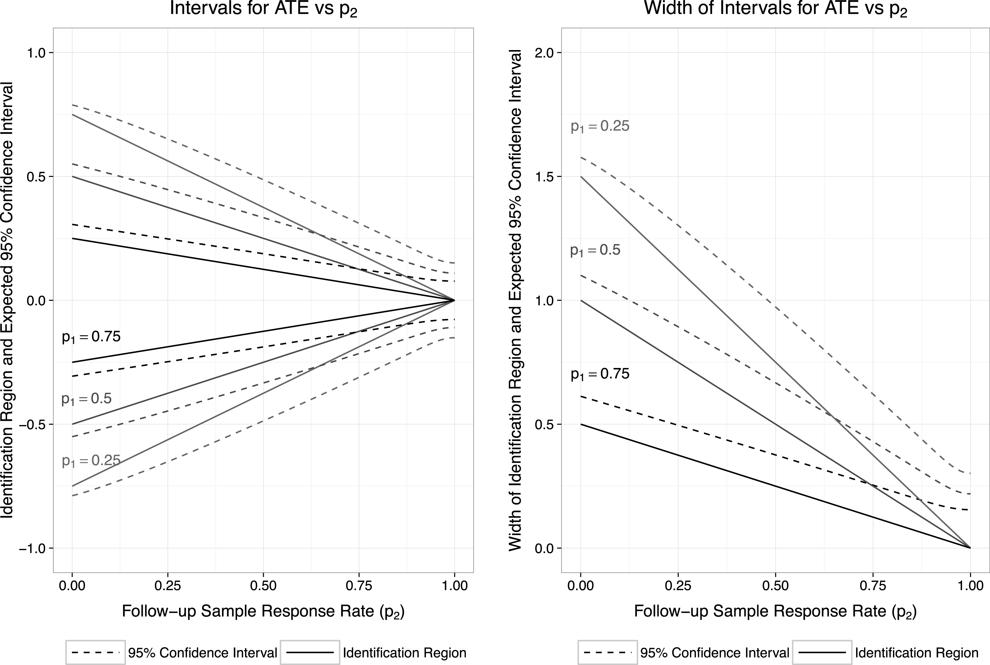
Figure 1 displays the results of our simulation. The left panel shows how the identification region and the
 $95\%$
confidence interval for the ATE respond to changes in
 $p_{2}$
. When
 $p_{2}$
is equal to zero, the intervals are the same as the worst-case intervals that would be obtained in the absence of double sampling. When
 $p_{2}$
is equal to
 $1$
– all subjects respond in the follow-up sample – the ATE is point-identified. We consider three scenarios, corresponding to an initial sample response rate of
 $0.25$
,
 $0.50$
, or
 $0.75$
. As the initial sample response rate increases, the identification region gets smaller. This pattern is more easily seen in the right panel, which plots the width of the identification region and associated confidence interval as a function of
 $p_{2}$
for each
 $p_{1}$
scenario. The lower the initial sample response rate, the wider the identification region. The width of this region shrinks to
 $0$
as the follow-up sample response rate increases.Footnote
14
4 Application
We replicate a survey experiment originally conducted by Levendusky and Malhotra (Reference Levendusky and Malhotra2016) that tested the effects of news stories on subjects’ policy views.Footnote 15 We conducted our replication on Amazon’s Mechanical Turk. Subjects could be exposed to one of three treatments: a “moderate” condition, in which subjects read an article describing the electorate as focused on finding common ground, a “polarized” condition, in which the article describes politics as contentious and the electorate as sharply divided, or a placebo condition (not analyzed here). The finding from the original experiment was that, compared to subjects in the moderate condition, subjects in the polarized condition reported more centrist policy positions but perceived typical partisans as holding more divergent views.
Our replication uses the identical experimental stimuli and outcome variables.Footnote 16 While the original experiment only collected immediate outcomes, our replications collected outcomes twice: immediately in a Wave 1 survey and again in a Wave 2 survey conducted 10 days later. The dependent variable, Perceived Polarization, is built from subjects’ responses to a series of policy questions. After giving their response to each question in the list below, subjects were asked how they think a “typical Democratic voter” and a “typical Republican voter” would respond to each question. The outcome variable is the average of the absolute values of the differences in subjects’ Democratic and Republican Responses.Footnote 17
(1) The tax rates on the profits people make from selling stocks and bonds, called capital gains taxes, are currently lower than the income tax rates many people pay. Do you think that capital gains tax rates should be increased, decreased, or kept about the same? (7 point scale. Decreased a lot: -3; Increased a lot: 3.)
(2) There is some debate about whether or not undocumented immigrants who were brought to this country illegally as children should be deported. Which of the following positions on the scale below best represents your position on this issue? (7 point scale. Very strongly oppose deportation: -3; Very strongly support deportation: 3.)
(3) The United States is currently considering signing additional free trade agreements with Central American, South American, and Asian countries. The Democratic Party wants to make it more difficult for the United States to enter into such agreements. The Republican Party wants to make it easier to do so. What do you think? Do you support or oppose the United States signing more free trade agreements with Central American, South American, and Asian countries? (7 point scale. Very strongly oppose free trade: -3; Very strongly support free trade: 3.)
(4) Public financing of elections is when the government pays for the cost of campaigning for various offices, rather than the campaigns relying on donations from the general public, corporations, or unions. Democrats typically support public financing plans while Republicans have wanted to eliminate them. What do you think? Do you support or oppose the government paying for the public financing of elections? (7 point scale. Very strongly oppose public financing: -3; Very strongly support public financing: 3.)
The estimand in this application is the sample ATE in wave 2 among those who participated in wave 1 of the experiment.
4.1 Attrition and double sampling
We encounter attrition when subjects who responded in Wave 1 fail to do so again in Wave 2. The “initial sample” refers to the first round of data collection in Wave 2 and the “follow-up sample” refers to the data collection effort among those selected for double sampling. Our experiment comprises 1,980 subjects, of which 1,444 had nonmissing responses in the initial sample.
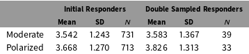
We assigned exactly 50 nonrespondents at random from each treatment group to the follow-up sample. While the initial compensation for the Wave 2 survey was $1.00, we offered selected nonrespondents $4.00 to participate. Of these 100 subjects, 72 completed the Wave 2 survey. Table 1 summarizes the number of subjects in each condition.
4.2 Results
Table 2 reports the average outcomes in each condition for subjects who initially responded in Wave 2 and for those who responded when offered additional incentives. A naive analysis (using the difference-in-means estimator only among those who responded in the first round) would conclude that the effect of the polarized condition was to raise average outcomes by
 $0.126$
(SE:
 $0.066$
, two-sided
 $p$
-value:
 $0.057$
). However, the naive estimator is only consistent if missingness is indeed ignorable. Table 2 also shows that the average outcomes in the initial and follow-up samples do not differ dramatically.
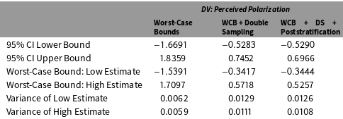
Table 3 illustrates what happens when we do not assume that missing outcomes are ignorable and use worst-case bounds instead. To estimate a lower bound on the ATE using responses only from Wave 2 without any double sampling, we replace missing outcomes in the Polarized group with the lowest possible values (
 $0$
) and missing outcomes in the Moderate group with the highest possible values (
 $6$
). To obtain an upper bound on the ATE, we reverse the procedure. The bounds, as expected, are so wide as to be of little probative value. The estimated bounds are
 $(-1.54,1.71)$
and the associated
 $95\%$
confidence interval equals
 $(-1.67,1.84)$
.
Attrition by treatment condition.

Outcome summaries by condition and response type.

Replication study results.

Our proposed method, double sampling combined with worst-case bounds, leads to dramatic reductions in the widths of the worst-case bounds and the associated
 $95\%$
confidence intervals. The relatively high response rates in the follow-up samples imply that fewer subjects receive worst-case imputations for their missing outcomes, so that worst-case bounds on the ATE are much more informative. The double sampling identification region for the ATE is estimated to be
 $(-0.34,0.57)$
. Adjusting for party identification by poststratification yields estimated bounds of
 $(-0.34,0.53)$
with an associated
 $95\%$
confidence interval equal to
 $(-0.53,0.70)$
. Whereas the width of the
 $95\%$
confidence interval using only the initial sample equals
 $3.50$
, double sampling with poststratification reduces it to
 $1.23$
, for a
 $65$
percent reduction in confidence interval width. This large decrease in interval width attests to the sharp reduction in fundamental uncertainty achieved by the double sampling design.
4.3 Sensitivity
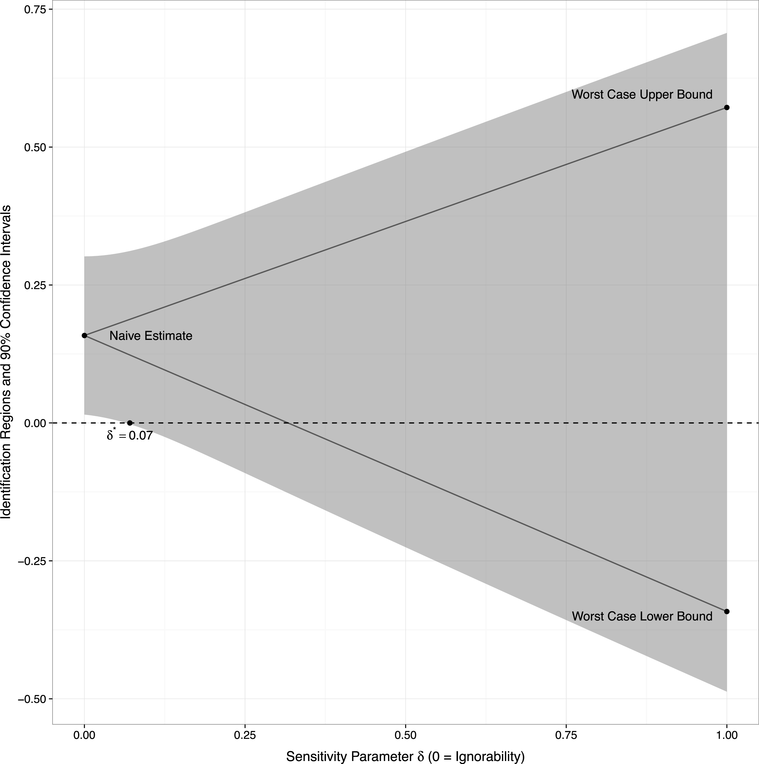
We implemented the sensitivity analysis described in Section 2.7. As shown in Figure 2, we obtain a
 $\unicode[STIX]{x1D6FF}^{\ast }$
of 0.07, implying that the statistically significant (at the
 $10\%$
level) naive estimate is very sensitive to even small violations of ignorability. If we conduct our sensitivity analysis at the
 $5\%$
level of statistical significance,
 $\unicode[STIX]{x1D6FF}^{\ast }$
does not exist, because the
 $95\%$
confidence interval around the naive estimate contains zero.
Sensitivity analysis.

5 Conclusion
We have proposed an approach for addressing missing outcome data in completely randomized experiments that makes fairly weak assumptions but may still yield substantively informative bounds on the ATE. Our approach is based on a combination of the double sampling design (Neyman Reference Neyman1938; Hansen and Hurwitz Reference Hansen and Hurwitz1946) and nonparametric worst-case bounds (Birnbaum and Sirken Reference Birnbaum and Sirken1950a,Reference Birnbaum and Sirkenb; Manski Reference Manski1990). We have shown that the resulting bounds on the ATE can be much narrower than the usual worst-case bounds from a single round of data collection. At the same time, our approach avoids the assumption that missingness is ignorable, at least after conditioning on observables. This ignorability assumption is credible in some but not all cases. The outcome stability assumption required by our approach provides an alternate identification assumption for researchers concerned about missing outcome data in their experiments. Finally, our approach can also complement the multiple imputation of missing outcomes, perhaps under the assumption that initial missingness is nonignorable but follow-up missingness is ignorable conditional on observables (Little and Rubin Reference Little and Rubin2002, ch. 15).
The advantages of our method are greatest when the initial outcome data collection generates inexpensive outcomes for a substantial fraction of experimental subjects and the follow-up data collection obtains outcomes for a large fraction of a random subsample of subjects with initially missing outcomes. As illustrated in our empirical application, fairly high success rates in the follow-up sample can often be achieved by concentrating significant effort and resources on a small number of subjects (see also An, Constantine, Beverly, and Constantin Reference An, Frangakis, Musick and Yiannoutsos2009, Jenkins, Scheim, Wang, Reed, and Green Reference Jenkins, Scheim, Wang, Reed and Green2004, and Fraser and Yan Reference Fraser and Yan2007). It is conceptually straightforward to combine double sampling with additional assumptions to further narrow the identification region (for examples of such a strategy see Manski and Nagin Reference Manski and Nagin1998, Manski and Pepper Reference Manski and Pepper2011, Mebane and Poast Reference Mebane and Poast2013, and Keele and Minozzi Reference Keele and Minozzi2013).
The approach proposed here can be generalized in various ways. For instance, it would be desirable to extend it to more complicated treatment assignment rules such as clustered random assignment, which introduce complications in variance estimation. It would also be useful to derive rules for optimal resource allocation along the lines of Hansen and Hurwitz (Reference Hansen and Hurwitz1946) for experimental designs that combine double sampling and worst-case bounds.
Supplementary material
For supplementary material accompanying this paper, please visit https://doi.org/10.1017/pan.2016.6.