2. Coordinate system and governing equations

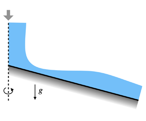
We adopt a standard spherical polar coordinate system taking the upward-directed axis of the cone as the polar axis (figure 1). The origin is placed at the cone tip; the distance from the origin is denoted by $r$ and the polar angle measured from the positive half of the polar axis by $\theta$. The surface of the cone is identified by $\theta = \beta$. A cone extending downward below the origin has $\beta > {{\rm \pi} }/{2}$; for $\beta ={{\rm \pi} }/{2}$, the cone surface degenerates into a horizontal plane. The polar angle of the film free surface is $\beta + \varPsi (r,t)$ so that, for a film flowing over the cone surface, $\varPsi <0$. It is convenient to introduce the reduced angular coordinate

(2.1)\begin{equation} \psi= \theta-\beta , \end{equation}

so that the film occupies the region $\varPsi (r,t) \leqslant \psi \leqslant 0$ and its surface is located at $\psi =\varPsi$.

Figure 1.

Geometry and coordinate system used in this paper; $r$ and $\theta$ are the spherical polar coordinates centred at the vertex of the cone with downward aperture $2({\rm \pi} -\beta )$; $\varPsi =\varPsi (r,t)$ and $h=h(r,t)$ are the angular and actual heights of the film surface above the cone surface.

The height of the film measured normally to the local cone surface is denoted by $h(r,t)$. It can be easily shown that the difference between $h$ and the arc length $r (-\varPsi )$ is of order $h^{2}/r^{2}$, i.e. of second order of smallness in the parameter $\epsilon$ to be defined shortly. Since the theory to be presented is accurate to first order in $\epsilon$, this small difference can be neglected. Thus, in the following, we set $h(r,t) = -r\varPsi (r,t)$.

In spherical polar coordinates the equation of continuity is

(2.2)\begin{equation} \frac{1}{r^{2}} \partial_r(r^{2}u) + \frac{1}{r \sin\theta} \partial_\theta (\sin\theta v) = 0 , \end{equation}

with $u$ and $v$ the velocity components in the radial and angular directions and $v>0$ when the velocity is directed toward the cone surface. The $\theta$- and $r$-momentum equations are

(2.3)\begin{align} \partial_tv + u \partial_r v + \frac{v}{r} \partial_\theta v+ \frac{u v}{r} &={-}\frac{1}{\rho r}\partial_\theta p +g \sin \theta \nonumber\\ & \quad +\nu\left[\frac{1}{r}\partial_r^{2}(r v) +\frac{1}{r^{2}} \partial_\theta^{2} v +\frac{\cot\theta}{r^{2} }\partial_\theta v +\frac{2}{r^{2}}\partial_\theta u - \frac{v}{r^{2}\sin^{2}\theta}\right] , \end{align}

and

(2.4)\begin{align} &\partial_t u+ u \partial_ru + \frac{v}{r}\partial_\theta u -\frac{v^{2}}{r} \nonumber\\ &\quad ={-} \frac{1}{\rho} \partial_rp -g\cos\theta + \nu \left[\frac{1}{r}\partial^{2}_r(ru) + \frac{1}{r^{2}} \partial_\theta^{2} u+\frac{\cot\theta}{r^{2}}\partial_\theta u -\frac{2}{r^{2}} \partial_\theta v -\frac{2}{r^{2}} u -\frac{2\cot\theta}{r^{2}}v\right] , \end{align}

respectively. Here, $p$ is the pressure, $g$ the acceleration due to gravity (positive downward) and $\rho$ and $\nu$ are the liquid density and kinematic viscosity, respectively.

At the free surface $\psi -\varPsi (r,t)=0$ the kinematic condition stipulates that

(2.5)\begin{equation} r\partial_t \varPsi = [v]_s - r[u]_s \partial_r \varPsi , \end{equation}

in which the subscript $s$ denotes evaluation at the free surface. Proceeding in a standard way, we now multiply (2.2) by $r^{2}\sin \theta \,{\rm d}\theta = r^{2}\sin \theta \,{\rm d}\psi$ and integrate from $\psi =0$ to $\psi =\varPsi$ to find

(2.6)\begin{equation} \partial_r \left(r^{2} \int_0^{\varPsi} \sin\theta u \,{\rm d}\psi\right) - r \sin (\beta+\varPsi) \left( r [u]_s \partial_r\varPsi - [v]_s\right) = 0 . \end{equation}

The first term is proportional to the volumetric flow rate $Q$ in the film,

(2.7)\begin{equation} q(r,t) \equiv \frac{Q}{2{\rm \pi}} ={-}r^{2} \int_0^{\varPsi} \sin\theta u \,{\rm d}\psi , \end{equation}

while the last two terms can be expressed in terms of $\partial _t\varPsi$ from (2.5). The result is, with $h=r(-\varPsi )$,

(2.8)\begin{equation} \partial_th+ \frac{1}{r\sin (\beta -h/r)} \partial_r q = 0 , \end{equation}

which is the standard relation expressing the time derivative of the film height as the divergence of the volumetric flow rate (see e.g. Oron, Davis & Bankoff Reference Oron, Davis and Bankoff1997; Leal Reference Leal2007). We have introduced a minus sign in the definition (2.7) of $Q$ to compensate for the fact that, here, $\varPsi <0$ as noted before. As defined, therefore, $Q>0$ when the flow is directed away from axis of the cone.

3. Scalings

The existing theories for the circular hydraulic jump make use of the boundary-layer approximation of the Navier–Stokes equations according to which inertia, pressure gradient and the part of the Laplacian normal to the boundary are of similar order (see e.g. Watson Reference Watson1964; Watanabe et al. Reference Watanabe, Putkaradze and Bohr2003). On the other hand, modelling of the flow down an inclined surface is usually carried out in the framework of what may be called the Kapitza scaling in which, to leading order, the streamwise component of gravity is primarily balanced by the normal Laplacian, inertia and pressure being of small order (see e.g. Kalliadasis et al. Reference Kalliadasis, Ruyer-Quil, Scheid and Velarde2012). The problem to be addressed here shares features of both situations, with the boundary-layer scaling relevant in the region of the hydraulic jump and the Kapitza scaling in the lower-velocity region downstream of the jump. We now consider these two situations and show that a single approximate form of the equations can be used for both situations as long as second-order errors are acceptable.

We start by scaling the coordinates and the dependent variables in a general way according to

(3.1a–f)\begin{equation} t \rightarrow \frac{L t}{U} ,\quad r\rightarrow Lr ,\quad \psi \rightarrow \frac{\delta}{L} \psi ,\quad u\rightarrow Uu ,\quad v\rightarrow Vv ,\quad p \rightarrow \Delta P \, p , \end{equation}

in which the velocity and pressure scales $U$, $V$ and $\Delta P$ will be specified as appropriate for each scaling, $\delta$ is of the order of the film thickness and $L$ is a characteristic length for the radial variable, assumed to be much larger than $\delta$. Upon substituting into the equation of continuity we find the familiar result

(3.2)\begin{equation} \frac{V}{U}=\frac{\delta}{L} \equiv \epsilon , \end{equation}

with $\epsilon \ll 1$. Since $\partial _\theta =\partial _\psi$, $\partial _\theta \rightarrow (1/\epsilon )\partial _\psi$ and the scaled equations become

(3.3)\begin{align}& \frac{1}{r^{2}}\partial_r(r^{2}u) +\frac{1}{r}\partial_\psi v + \epsilon \frac{\cot\theta}{ r}v =0 , \end{align}

(3.4)\begin{align} &\epsilon^{2}\left( \partial_tv+ u \partial_r v + \frac{v}{r} \partial_\psi v+ \frac{u v}{r}\right)\nonumber\\ &\quad ={-}\frac{\Delta P}{\rho U^{2} r} \partial_\psi p + \epsilon \frac{Lg} {U^{2}}\sin \theta \nonumber\\ &\qquad +\frac{\nu}{LU} \left[ \epsilon^{2} \frac{1}{r}\partial_r^{2}(r v) + \frac{1}{r^{2}} \partial_\psi^{2} v + \frac{ \epsilon\cot\theta}{ r^{2} }\partial_\psi v + \frac{2}{ r^{2}}\partial_\psi u - \epsilon^{2} \frac{v}{r^{2}\sin^{2}\theta}\right], \end{align}

and

(3.5)\begin{align} & \epsilon^{2}\left( \partial_t u+ u \partial_ru + \frac{v}{r}\partial_\psi u -\epsilon^{2}\frac{v^{2}}{r} \right) \nonumber\\ &\quad ={-} \epsilon^{2} \frac{\varDelta P}{\rho U^{2}} \partial_rp -\epsilon^{2} \frac{Lg}{U^{2}}\cos\theta \nonumber\\ & \qquad + \frac{\nu}{LU} \left[\epsilon^{2}\frac{1}{r}\partial^{2}_r(ru) + \frac{1}{r^{2}} \partial_\psi^{2} u +\epsilon \frac{ \cot\theta}{r^{2}}\partial_\psi u - \epsilon^{2}\frac{2}{ r^{2} } \partial_\psi v -\frac{2\epsilon^{2}}{r^{2}} u-2\epsilon^{3}\frac{\cot\theta}{r^{2}}v\right] . \end{align}

As long as $\epsilon$ is small, the terms multiplied by $\epsilon ^{2}$ and $\epsilon ^{3}$ in the viscous contributions on the right-hand side of these equations will always be small compared with the other ones and can be dropped. Furthermore, since $|\psi | \sim h/r \sim \epsilon$, terms proportional to $\epsilon \cot \theta$ can be replaced by $\epsilon \cot \beta$ with an $O(\epsilon ^{2})$ error. The same approximation can be applied to the equation of continuity which then becomes

(3.6)\begin{equation} \frac{1}{r^{2}}\partial_r(r^{2}u) +\frac{1}{r}\partial_\psi v + \epsilon \frac{\cot\beta}{ r}v =0 . \end{equation}

For the Kapitza scaling we let

(3.7a,b)\begin{equation} U = \frac{g\delta^{2}}{\nu} , \quad \Delta P = \rho g \delta . \end{equation}

Up to a numerical factor, the velocity scale is of the order of the mean Nusselt velocity for the flow of a flat film down a vertical solid plane while the pressure scale expresses the dominance of hydrostatic effects. In principle these scales should be adjusted according to the inclination of the solid surface but, here, the aperture of the cone is an important parameter which should not be hidden in the normalization. With these choices, the equation of continuity maintains the form (3.6) and the $\psi$ (or $\theta$) momentum equation becomes

(3.8)\begin{align} \epsilon^{2}\left(\partial_tv+ u \partial_r v + \frac{ v}{r} \partial_\psi v+ \frac{u v}{r}\right)&={-}\frac{\nu^{2} }{g \delta^{3} } \left(\frac{1}{r} \partial_\psi p - \sin \theta \right) \nonumber\\ & \quad +\epsilon \frac{\nu^{2}}{g\delta^{3} } \frac{1}{r^{2}}\left( \partial_\psi^{2} v + 2\partial_\psi u + \epsilon\cot\beta \partial_\psi v \right) . \end{align}

This equation explicitly shows the dominant balance of gravity and pressure gradient normal to the solid surface, with viscous effects minor and inertia of secondary importance. After division by $\epsilon$, the $r$ momentum equation becomes

(3.9)\begin{equation} \epsilon\left( \partial_tu+ u \partial_ru + \frac{v}{r}\partial_\psi u\right) ={-}\frac{\nu^{2} }{g \delta^{3}} \left(\cos \theta +\epsilon \partial_rp \right) +\frac{\nu^{2}}{g\delta^{3} } \frac{1}{r^{2}}\left( \partial_\psi^{2} u +\epsilon \cot\beta \partial_\psi u \right) . \end{equation}

The dimensionless group $g\delta ^{3}/\nu ^{2}$ can be written as $\delta U/\nu$ and is seen therefore to play the role of a Reynolds number based on the film thickness. In order to reflect, to leading order, the dominant balance between streamwise gravity and viscosity characteristic of film flow down an inclined plane, it is evident that this Reynolds number must be of order 1 or smaller.

For the boundary-layer scaling we assume that the velocity scale $U$ is imposed by some external agent, such as the jet that causes the hydraulic jump, and that the pressure scale is $\Delta P=\rho U^{2}$ as in normal boundary-layer theory. The $\psi$ momentum equation becomes

(3.10)\begin{align} \epsilon^{2}\left( \partial_tv+ u \partial_r v + \frac{v}{r} \partial_\psi v+ \frac{u v}{r}\right) &={-} \frac{1}{r}\partial_\psi p +\frac{1}{Re} \frac{1}{r^{2}}\left( \partial_\psi^{2} v + 2\partial_\psi u + \epsilon\cot\beta \partial_\psi v \right) \nonumber\\ &\quad +\frac{\epsilon Lg} {U^{2}}\sin \theta , \end{align}

in which $Re=UL/\nu$ is the Reynolds number, and the $r$ momentum equation

(3.11)\begin{equation} \epsilon^{2}Re\left( \partial_tu+ u \partial_ru + \frac{v}{r}\partial_\psi u \right) ={-} \epsilon^{2}Re \, \partial_rp + \frac{1}{r^{2}}\left( \partial_\psi^{2} u +\epsilon \cot\beta \partial_\psi u\right) - \epsilon^{2}Re \frac{ Lg}{U^{2}}\cos\theta . \end{equation}

The standard form of the boundary-layer equations is recovered upon taking $Re=O(\epsilon ^{-2})$. Equation (3.10) shows then that inertial and viscous contributions to the normal pressure gradient are of second order while, in order to have a physically significant balance, it is necessary to assume $Lg/U^{2} \sim O(1/\epsilon )$. From this remark, the $r$-momentum equation then shows that this boundary-layer scaling is only appropriate provided $\cos \theta \sim O(\epsilon )$. This conclusion can be restated in a more interesting way: in order for the streamwise pressure to have the same order of magnitude as inertia and viscosity, which is a necessary condition for the existence of a hydraulic jump, it is necessary that the inclination of the solid surface be small. The results to be presented later will confirm this conclusion.

As already stated, we will work correct to $O(\epsilon )$. Upon dropping all $O(\epsilon ^{2})$ terms from the Kapitza form of the momentum equations we have (3.9) and

(3.12)\begin{equation} - \frac{1}{r} \partial_\psi p + \sin \theta + \frac{\epsilon}{r^{2}} \left( \partial_\psi^{2} v + 2\partial_\psi u \right) =0 , \end{equation}

while the boundary-layer form becomes, with $\epsilon ^{2} Re=1$,

(3.13)\begin{equation} - \frac{1}{r} \partial_\psi p + \frac{\epsilon Lg} {U^{2}}\sin \theta =0 , \end{equation}

and

(3.14)\begin{equation} \partial_tu+ u \partial_ru + \frac{v}{r}\partial_\psi u ={-} \partial_rp + \frac{1}{r^{2}}\partial_\psi^{2} u -\frac{ \epsilon Lg}{U^{2}} \frac{\cos\theta }{\epsilon} . \end{equation}

In the last equation we have explicitly used the fact that, for consistency, $\epsilon Lg/U^{2}$ must be of order 1 so that $\cos \theta = \cos (\beta +\psi ) =\cos \beta +O(\epsilon )$ must be of order $\epsilon$. This remark also implies that terms proportional to $\epsilon \cot \beta$ in the momentum and continuity equations are of order $\epsilon ^{2}$ and can, therefore be omitted. For the boundary-layer scaling, therefore, the equation of continuity simplifies to

(3.15)\begin{equation} \frac{1}{r^{2}}\partial_r(r^{2}u) +\frac{1}{r}\partial_\psi v =0 . \end{equation}

A consideration of the equations of continuity (3.6) and (3.15) in the two scalings shows that the two differ by the term $\epsilon (\cot \beta ) \,v/r$. Only the inertial term in the Kapitza $r$ momentum equation (3.9) is affected if this difference is disregarded but, since this term is of order $\epsilon$, the error thus introduced is of an inconsequential order $\epsilon ^{2}$. The boundary-layer form of the continuity and $\psi$ momentum equations can therefore be used when either scaling is appropriate. On a similar basis, the difference between the pressures in the two scaling arises from the $\epsilon$ term in the Kapitza $\psi$ momentum equation (3.12) and enters the $r$ momentum equation (3.9) where the pressure gradient is multiplied by $\epsilon$, thus introducing another negligible contribution of order $\epsilon ^{2}$ if the boundary-layer form (3.13) is used. Furthermore, $\sin \theta = \sin (\beta +\psi ) = \sin \beta \cos \psi + \cos \beta \sin \psi = \sin \beta +O(\epsilon )$ with the Kapitza scaling, while $\sin \theta = \sin \beta +O(\epsilon ^{2})$ with the boundary-layer scaling since $\cos \beta =O(\epsilon )$. Thus, with either scaling, we can consistently approximate (3.12) and (3.13) by

(3.16)\begin{equation} - \frac{1}{r}\partial_\psi p + \frac{\epsilon Lg} {U^{2}}\sin \beta =0 , \end{equation}

or the equivalent form with the Kapitza scaling. The two radial momentum equations differ by the presence of the term $\epsilon (\cot \beta /r^{2}) \partial _\psi u$ in the Kapitza form. This term will, however, be of order $\epsilon ^{2}$ and, therefore, negligible when the boundary-layer scaling is appropriate and it can therefore be retained without significant error. Thus we conclude that a mathematical model consistent with both scalings can be built from the continuity and $\psi$ momentum equations of the boundary-layer scaling, together with the $r$ momentum equation of the Kapitza scaling.

Returning to the unscaled form, therefore, the equations to be considered are (3.15) and

(3.17)\begin{equation} - \frac{1}{r} \partial_\psi p + \rho g \sin \beta =0 , \end{equation}

and

(3.18)\begin{equation} \partial_tu+ u \partial_ru + \frac{v}{r}\partial_\psi u ={-} \frac{1}{\rho} \partial_rp + \frac{\nu}{r^{2}}\left( \partial_\psi^{2} u +\cot\beta \partial_\psi u\right) -g\cos\theta . \end{equation}

In the language of singular perturbations theory we can describe the previous analysis and conclusion by stating that the Kapitza and boundary-layer scalings are two distinguished limits of the scaled equations (3.4) and (3.5). The final system with which we will be concerned, namely (3.15), (3.17) and (3.18), is then the set of composite equations valid in both distinguished limits according to the extension theorem of singular perturbation theory (see e.g. Lagerstrom & Casten Reference Lagerstrom and Casten1972).

3.1. Boundary conditions

With the free surface defined by $\psi - \varPsi (r,t) = 0$ as before, the unit normal is given by

(3.19)\begin{equation} \boldsymbol{n} = \frac{-r\partial_r\varPsi \boldsymbol{e}_r +\boldsymbol{e}_\theta}{\sqrt{1+(r\partial_r\varPsi)^{2}}} \simeq{-}r\partial_r\varPsi \boldsymbol{e}_r +\boldsymbol{e}_\theta , \end{equation}

with $\boldsymbol {e}_r$ and $\boldsymbol {e}_\theta$ unit vectors in the coordinate directions. Consistent to first order in $\varPsi$, the square root in this expression can be approximated by 1, which implies that the slope of the free surface is small so that the last step is accurate to the order of $O(\epsilon )$. As we will see, it is possible that this approximation contributes some error in the neighbourhood of a hydraulic jump on a horizontal surface, but the effect remains localized (see e.g. figure 12). The unit tangent $\boldsymbol {t}$ to the free surface is $\boldsymbol {t}=(\boldsymbol {e}_r, r\partial _r\varPsi \boldsymbol {e}_\theta )+O(\epsilon ^{2})$. The curvature $\mathcal {C}$ of the free surface is approximately given by

(3.20)\begin{equation} {\mathcal{C}} = \left[\boldsymbol{\nabla}\boldsymbol{\cdot}\boldsymbol{n}\right]_{\psi=\varPsi} \simeq \frac{\cot(\beta+\varPsi)}{r} -\frac{1}{r^{2}}\partial_r(r^{3}\partial_r\varPsi) . \end{equation}

The two terms are of the same order when $\cot \beta =O(\epsilon )$, but the second one is of order $\epsilon$ compared with the first one when $\cot \beta =O(1)$. To $O(\epsilon )$, in terms of $h$, this equation is

(3.21)\begin{equation} {\mathcal{C}} \simeq \frac{\cot\beta}{r} +\frac{h}{r^{2}\sin^{2}\beta} +\frac{1}{r^{2}}\partial_r\left(r^{3}\partial_r \frac{h}{r}\right) . \end{equation}

When the medium above the film has a constant pressure $p_a$ but otherwise negligible dynamical effects, which we assume, the dynamic condition requires that the stress tangent to the free surface vanishes. It is readily shown that, correct to $O(\epsilon )$, this condition simply implies that

(3.22)\begin{equation} \frac{1}{r}\partial_\psi u = 0 , \end{equation}

which is a standard condition in thin-film analysis (see e.g. Bohr et al. Reference Bohr, Dimon and Putkaradze1993; Oron et al. Reference Oron, Davis and Bankoff1997; Ruyer-Quil & Manneville Reference Ruyer-Quil and Manneville1998, Reference Ruyer-Quil and Manneville2000; Watanabe et al. Reference Watanabe, Putkaradze and Bohr2003). With ${\mathcal {C}}^{*}=L{\mathcal {C}}$, for the Kapitza scaling, the dynamic condition on the normal stress can be written as

(3.23)\begin{equation} -p^{*} +2\epsilon \left( \frac{1}{ r^{*} }\partial_{\psi^{*}} v^{*}+ \frac{u^{*}}{r^{*}} - \partial_{r^{*}}\varPsi^{*}\partial_{\psi^{*}} u^{*}\right) ={-} p_a^{*}+ \frac{\sigma}{ \rho g \delta L} {\mathcal{C}}^{*} , \end{equation}

where $\sigma$ is the surface-tension coefficient and we temporarily use asterisks to denote normalized variables. According to (3.9), the $O(\epsilon )$ terms give an $O(\epsilon ^{2})$ contribution to the $r$ momentum equation and are therefore negligible. In order to retain the effect of surface tension it is necessary to assume that $\sigma /(\rho g \delta L) = O(1)$. With the boundary-layer scaling, the condition is

(3.24)\begin{equation} - p^{*} + \frac{2}{Re } \left( \frac{1}{ r^{*} }\partial_{\psi^{*}} v^{*}+ \frac{u^{*}}{r^{*}} - \partial_{r^{*}}\varPsi^{*} \partial_{\psi^{*}} u^{*}\right) ={-}p_a^{*}+ \frac{\sigma}{\rho U^{2}L} {\mathcal{C}}^{*} , \end{equation}

and, given that $Re=O(\epsilon ^{-2})$, the term in parentheses is negligible. Surface tension remains a non-negligible force if $\sigma /(\rho U^{2}L)=O(1)$. Thus we see that, for both cases, the normal stress condition reduces to the dimensional form

(3.25)\begin{equation} p =p_a- \sigma {\mathcal{C}} . \end{equation}

At the solid surface $\psi =0$ the no-slip condition applies.

4. Approximate equation for the film thickness

Starting with Tani (Reference Tani1949), several authors have pointed out that, approximately, the location of the hydraulic jump can be determined on the basis of a simplified first-order equation for the film height derived for steady flow. We take a different approach and start by deriving an equation for time-dependent flow reducing it to the steady case at the appropriate moment.

Rather than following the von Kármán–Pohlhausen method used in earlier studies (Tani Reference Tani1949; Watson Reference Watson1964; Watanabe et al. Reference Watanabe, Putkaradze and Bohr2003), in our derivation we adapt to the present situation the Galerkin method developed by Ruyer-Quil & Manneville (Reference Ruyer-Quil and Manneville1998, Reference Ruyer-Quil and Manneville2000) for the two-dimensional case, which has proven very effective in that case. The approximate results to be derived here will be supported by the numerical solutions of the full Navier–Stokes equations.

Upon integrating (3.17) we find

(4.1)\begin{equation} p = p_a+ \rho g \sin \beta r (\psi -\varPsi) -\sigma {\mathcal{C}} . \end{equation}

This relation can now be substituted into the $r$-momentum equation (3.18) to find

(4.2)\begin{align} \partial_t u+ u\partial_r u + \frac{v}{r}\partial_\psi u &= g\sin\beta (\varPsi+r\partial_r \varPsi) +\frac{\sigma}{\rho} \partial_r{\mathcal{C}} \nonumber\\ &\quad +\frac{\nu}{r^{2}}( \partial_\psi^{2} u +\cot\beta \partial_\psi u) - g \cos \beta , \end{align}

in which we have expanded $g\cos \theta = g\cos (\beta +\psi )$ correctly to first order in the last term.

We now write the radial velocity in the similarity form used by many earlier authors (see e.g. Watson Reference Watson1964; Watanabe et al. Reference Watanabe, Putkaradze and Bohr2003), which, in our case, is

(4.3)\begin{equation} u = \frac{\psi}{\varPsi} \left(2 - \frac{\psi}{\varPsi}\right)V(r,t) , \end{equation}

with the surface radial velocity $V(r,t)$ to be determined by relating $u$ to the volumetric flow rate of the film as shown below. It may be noted that (4.3) satisfies no slip at the wall and zero tangential stress on the free surface as per (3.22). In the spirit of the Galerkin method we multiply (4.2) by $u$ and integrate over the film thickness

(4.4)\begin{align} &\int_0^{\varPsi} u \partial_tu \,{\rm d}\psi+ \int_0^{\varPsi} u\left( u\partial_r u + \frac{v}{r}\partial_\psi u \right){\rm d}\psi\nonumber\\ &\quad= \frac{\nu}{r^{2}} \int_0^{\varPsi} u \left(\partial_\psi^{2} u + \cot \beta \partial_\psi u\right) {\rm d}\psi + \left[[\sin\beta \partial_r(r\varPsi) -\cos\beta]g+\frac{\sigma}{\rho}\partial_r{\mathcal{C}}\right] \int_0^{\varPsi} u \,{\rm d}\psi . \end{align}

Use of the equation of continuity in the simplified boundary-layer form (3.15), of the kinematic boundary condition (2.5), of the shear stress condition (3.22) and integration by parts permit us to rewrite the previous equation to gain some physical understanding at the same time simplifying somewhat the calculations

(4.5)\begin{align} \frac{1}{2}\partial_t \int_0^{\varPsi} u^{2} \,{\rm d}\psi+ \frac{1}{2r^{2}} \partial_r \left( r^{2} \int_0^{\varPsi} u^{3} \,{\rm d}\psi \right) &= \left( g[ \sin\beta \partial_r(r\varPsi) -\cos\beta] +\frac{\sigma}{\rho} \partial_r{\mathcal{C}}\right)\int_0^{\varPsi} u \,{\rm d}\psi \nonumber\\ & \quad +\frac{\nu}{r^{2}}\left( - \int_0^{\varPsi} (\partial_\psi u)^{2}\,{\rm d}\psi +\frac{1}{2} \cot \beta [u^{2}]_s \right). \end{align}

To $O(\epsilon )$, this will be recognized as the integral form of the kinetic energy balance for the liquid. The first and second terms on the left-hand side are the rate of change of the kinetic energy and the divergence of the kinetic energy flow rate. On the right-hand side, the first term is the integral of $-\boldsymbol {\nabla } \boldsymbol {\cdot} (p\boldsymbol {u}/\rho )+\boldsymbol {u}\boldsymbol {\cdot}\boldsymbol {g} = \boldsymbol {u}\boldsymbol {\cdot}(- \boldsymbol {\nabla } p/\rho +\boldsymbol {g})$ and the second one the integral of the dissipation function. Again using $\varPsi = -h/r$, after substitution of u by V, integration and multiplication by $-r^{2}$, the final result may be written as

(4.6)\begin{align} &\frac{4}{15} \partial_t\left(rhV^{2} \right) +\frac{8}{35} \partial_r \left(rh V^{3}\right) \nonumber\\ & \qquad = \frac{2}{3} rhV \left[{-}g( \sin\beta \partial_r h + \cos\beta) + \frac{\sigma}{\rho} \partial_r{\mathcal{C}}\right] -\frac{4}{3} \nu \frac{r}{h} V^{2} \left(1+\frac{3}{8}\cot \beta \frac{h}{r}\right) . \end{align}

It is convenient to rewrite this equation in terms of the volumetric flow rate $q=Q/2{\rm \pi}$ because this quantity is a constant in steady conditions. Expanding $\sin \theta$ to first order in the definition (2.7) of $q$ we have

(4.7)\begin{equation} q \simeq{-} r^{2} \int_0^{\varPsi} (\sin \beta +\cos \beta \psi) u \,{\rm d}\psi = \frac{2}{3} rh V \sin \beta\left(1-\frac{5}{8}\cot \beta \frac{h}{r} \right) , \end{equation}

from which

(4.8)\begin{equation} V = \frac{3 q}{2rh \sin\beta} \left[1+\frac{5}{8}\cot \beta \frac{h}{r} + O\left(\frac{h^{2}}{r^{2}}\right)\right] . \end{equation}

An examination of the order of magnitude of the terms in (4.6) shows that it is consistent to retain the $O(h/r)$ term of this relation only in the viscous term on the right-hand side. Furthermore, the $\partial _th$ terms can be expressed in terms of the volumetric flux $q$ by using the integrated continuity equation (2.8) which, itself, can be expanded to read

(4.9)\begin{equation} \partial_t h + \frac{1}{r\sin\beta}\left(1+ \cot\beta \frac{h}{r}\right) \partial_r q=0 . \end{equation}

With this step, correct to $O(h/r)$, the integral form (4.6) of the momentum equation becomes

(4.10)\begin{align} & \partial_t q +\frac{17}{7} \frac{q}{hr \sin \beta } \partial_r q - \frac{5}{6}\left( \frac{54}{35} \frac{q^{2}}{h^{2} r\sin\beta } -g hr\sin^{2}\beta \right) \partial_rh \nonumber\\ & \quad ={-}\frac{5}{6} hr\sin\beta \left(g\cos\beta - \frac{\sigma}{\rho }\partial_r{\mathcal{C}}\right) +\frac{9}{7} \frac{q^{2}}{h r^{2}\sin\beta} - \frac{5}{2}\frac{\nu q}{h^{2} } \left(1+\cot\beta \frac{h}{r} \right) . \end{align}

This equation, together with (4.9), or its original form (2.8), which relates the film thickness to the volumetric flow rate, constitutes a two-equation model for the time-dependent evolution of the film.

It is interesting to relate this result to the form derived by Ruyer-Quil & Manneville (Reference Ruyer-Quil and Manneville2000) for two-dimensional flow down an inclined plate, as this equation has been shown to be optimal at first order (Kalliadasis et al. Reference Kalliadasis, Ruyer-Quil, Scheid and Velarde2012, p. 168). This objective can be achieved by identifying $Q/(2{\rm \pi} r\sin \beta ) = q/(r\sin \beta )$ with the two-dimensional flow rate $q_{2D}$ and by taking the limit $r\rightarrow \infty$. The first step is necessary because $Q$ is the flow rate through a circular surface of radius $r\sin \beta$ so that $Q/(2{\rm \pi} r\sin \beta )$ is the flow rate per unit width. The second one reflects the fact that, as $r \rightarrow \infty$, the effect of the cone curvature becomes smaller and smaller approaching a flat surface. With these steps, after writing $x$ in place of $r$, (4.9) becomes

(4.11)\begin{equation} \partial_t h+ \partial_x q_{2D} = 0 , \end{equation}

while (4.10) becomes

(4.12)\begin{align} & \partial_t q_{2D} +\frac{17}{7} \frac{q_{2D}}{h } \partial_x q_{2D} - \frac{5}{6}\left( \frac{54}{35} \frac{q_{2D} ^{2}}{h^{2}} -g h\sin \beta \right) \partial_xh \nonumber\\ & \qquad ={-}\frac{5}{6} h \left(g\cos\beta - \frac{\sigma}{\rho } \partial_x {\mathcal{C}}\right) - \frac{5}{2}\frac{\nu }{h^{2} }q_{2D} , \end{align}

with ${\mathcal {C}} = \partial _x^{2}h$. This is precisely the first-order model for two-dimensional flow of a thin film over an inclined plate derived in Ruyer-Quil & Manneville (Reference Ruyer-Quil and Manneville2000). In steady conditions $\partial _th=0$ so that $\partial _x q_{2D}=0$ and the second equation becomes

(4.13)\begin{equation} \left( \frac{54}{35} \frac{q_{2D} ^{2}}{h^{2}} -g h\sin \beta \right) \frac{{\rm d}h}{{\rm d}\kern0.06em x} = \left(g\cos\beta - \frac{\sigma}{\rho }\frac{{\rm d}{\mathcal{C}}}{{\rm d}\kern0.06em x}\right)h+3\frac{\nu }{h^{2} }q_{2D} . \end{equation}

If the inclination to the horizontal is denoted by $\eta$, then $\beta = \frac {{\rm \pi} }{2} + \eta$ so that $\cos \beta = -\sin \eta$. This equation then possesses a uniform solution in which the film thickness is related to the flow rate according to the well-known Nusselt result (see e.g. Chang & Demekhin Reference Chang and Demekhin2002; Kalliadasis et al. Reference Kalliadasis, Ruyer-Quil, Scheid and Velarde2012)

(4.14)\begin{equation} q_{2D} = \frac{gh^{3} \sin \eta}{3 \nu} . \end{equation}

5. First-order equation for steady flow

In steady conditions $\partial _th=0$ and $\partial _tq=0$ so that (4.9) simply states that $q$ is constant. Using this fact in (4.10) and dropping the surface-tension term $\partial _r{\mathcal {C}}$, we obtain the first-order equation

(5.1)\begin{align} & \left(\frac{54}{35} \frac{q^{2}}{r^{2}\sin^{2}\beta} -g h^{3}\sin\beta \right) \frac{{\rm d}h}{{\rm d}r} \nonumber\\ & \quad =h^{3}g\cos\beta -\frac{54}{35} \frac{hq^{2}}{ r^{3}\sin^{2}\beta } +\frac{3\nu q}{r \sin\beta} \left(1+\cot\beta \frac{h}{r} \right) . \end{align}

For $\beta ={{\rm \pi} }/{2}$ a similar equation has been derived by many authors. In all cases the groups of dimensional terms have the same structure, namely $gh^{3}$, $q^{2}/r^{2}$ etc., and they carry the same signs, but the numerical coefficients are different. Since, as already noted, (5.1) reduces to the optimal two-dimensional equation in the appropriate limit, we believe that our coefficients are preferable. There is only one previous study which includes a small deviation of the plate from planarity (Kasimov Reference Kasimov2008). In that study the equation analogous to (5.1) is written as

(5.2)\begin{equation} \left(\frac{6q^{2}}{5r^{2}}-gh^{3} \right)\frac{{\rm d}h}{{\rm d}r} = s_b gh^{3}+\frac{3\nu q}{r} -\frac{6q^{2}h}{5r^{3}}, \end{equation}

in which $s_b$ is the plate slope, assumed to be small; in our notation, $s_b= \tan ({{\rm \pi} }/{2}-\beta )$. For angles close to $90^{\circ }$ this equals $\sin ({{\rm \pi} }/{2}-\beta )=\cos \beta$ and $\sin \beta \simeq 1$, so that (5.2) and (5.1) agree in this limit of small inclination except for the coefficient $\frac {54}{35}\simeq 1.543$ replacing $\frac {6}{5}=1.2$.

For future reference it may be pointed out that, for large $r$, (5.1) has the approximate solution

(5.3)\begin{equation} h \simeq \left(\frac{3\nu q}{g \sin \beta (-\cos\beta)r}\right)^{1/3} , \end{equation}

in agreement with the result of Zollars & Krantz (Reference Zollars and Krantz1980). We have verified that the additional terms that we can calculate from (5.1) agree with those given in Zollars & Krantz (Reference Zollars and Krantz1980). Since the method used by these authors is very different from the present one, agreement of the present results with the numerical coefficients that they found lends further support to the correctness of our derivation.

The expression (5.3) may be considered as the three-dimensional analogue of the Nusselt solution (4.14) and describes a situation in which gravity balances viscosity even though the film thins by continuity due to the diverging nature of the cone surface area. It is evident that (5.3) becomes meaningless as $\cos \beta \rightarrow 0$ as, in that case, gravity cannot assist in generating a flow of the film. The absence of an asymptotic solution of equations of the form (5.1) for $\beta =90^{\circ }$ has been proven and discussed earlier in Bohr et al. (Reference Bohr, Dimon and Putkaradze1993).

6. Conditions for the numerical simulations

The direct numerical simulations are carried out with the open-source software OpenFOAM v2012, as described in Appendix C. These simulations require a boundary condition at the right end of the domain. In order to minimize the effect of these conditions on the steady-state solution in which we are mostly interested, following Fernandez-Feria et al. (Reference Fernandez-Feria, Sanmiguel-Rojas and Benilov2019) and Wang & Khayat (Reference Wang and Khayat2021), we simulate the free fall of the film down a vertical solid surface attached to the end of the inclined cone surface, as shown in figure 15.

Figure 2 compares our predictions of the hydraulic jump phenomenon against the experimental data by Duchesne et al. (Reference Duchesne, Lebon and Limat2014). Silicon oil (with density $960\ {\rm kg}\ {\rm m}^{-3}$, kinematic viscosity $2\times 10^{-5}\ {\rm m}^{2}\ {\rm s}^{-1}$ and surface-tension coefficient $0.02\ {\rm N}\ {\rm m}^{-1}$) is injected downward from a 1.6 mm-radius round nozzle onto a horizontally placed circular disk with a radius of 15 cm. The volumetric flow rate is $17\ {\rm cm}^{3}\ {\rm s}^{-1}$. The inlet is placed 4.8 mm above the plate. As shown in Brechet & Néda (Reference Brechet and Néda1999), this nozzle-to-wall distance has little influence on the position of the hydraulic jump. One observes a close agreement between experiment and simulations, which supports the accuracy of the latter.

Figure 2.

Comparison of the free-surface profile normalized by the jet radius, $h/a$, as given by the present Navier–Stokes simulations (solid line) with the data of Duchesne, Lebon & Limat (Reference Duchesne, Lebon and Limat2014) (symbols).

Figure 3 shows a comparison of our numerical results for different jet flow rates $Q$ (closed circles and squares) with some experiments of Hansen et al. (Reference Hansen, Hørlück, Zauner, Dimon, Ellegaard and Creagh1997) for water (open circles) and an oil with a kinematic viscosity 15 times that of water (open squares). The solid lines are the predictions of the inertial lubrication theory of Rojas et al. (Reference Rojas, Argentina, Cerda and Tirapegui2010) while the dashed lines are just guides to the eyes. The agreement with the oil data is quite good. That with the water data less so, although our results are in very close agreement with those of Rojas et al. (Reference Rojas, Argentina, Cerda and Tirapegui2010). It may also be noted that Hansen et al. (Reference Hansen, Hørlück, Zauner, Dimon, Ellegaard and Creagh1997) state that the radius of the jump was oscillating for $Q$ greater than approximately $15\ {\rm cm}^{3}\ {\rm s}^{-1}$ so that the data shown are mean values. Since the unsteadiness mentioned by Hansen et al. was not observed in our simulation, it is possible that it was caused by the specific experimental system used. Some additional considerations on this comparison can be found in the supplementary material associated with this paper available at https://doi.org/10.1017/jfm.2022.777.

Figure 3.

Comparison of our Navier–Stokes simulations (solid symbols) for the jump radius with those reported in Hansen et al. (Reference Hansen, Hørlück, Zauner, Dimon, Ellegaard and Creagh1997) (open symbols). Results for water are denoted by circles, those for oil by squares. The grey lines are the prediction of the model developed by Rojas et al. (Reference Rojas, Argentina, Cerda and Tirapegui2010). The jump radius is identified with the position of the point of maximum curvature as shown in the insets (not to scale).

Finally, a comparison with the numerical results of Fernandez-Feria et al. (Reference Fernandez-Feria, Sanmiguel-Rojas and Benilov2019), included in Appendix C, is in excellent agreement with the reported results.

Most of the simulations below refer to the case of a jet Reynolds number $Re_j=2a Q/({\rm \pi} a^{2} \nu ) \simeq 152.8$ with $a$ the radius of the impinging jet. For a silicon oil with $\nu =50\times 10^{-6}\ {\rm m}^{2} {\rm s}^{-1}$ and a radius $a = 2.5$ mm, this value of $Re_j$ would correspond to a flow rate $Q=30\times 10^{-6}\ {\rm m}^{3}\ {\rm s}^{-1}$. The jet is introduced with a uniform velocity profile at a height equal to $3a$. The length of the computational domain is $24a$, although in many figures only a portion of length $16a$, which is little influenced by the right boundary condition, is shown. The height of the vertical section at the right end of the domain is $2a$ and free outflow conditions are imposed at the exit of the domain. Unless otherwise specified, the Bond number is $Bo=\rho g a^{2}/\sigma$ = 2.83 with, e.g. $\rho = 970\ {\rm kg}\ {\rm m}^{-3}$ and $\sigma =0.021\ {\rm N}\ {\rm m}^{-1}$.

Watson (Reference Watson1964) pointed out that the film generated by a circular jet falling vertically on a horizontal plate reaches a minimum thickness $h_m$ upstream of the jump. We compared Watson's estimates of this minimum thickness and of its location with the results of our Navier–Stokes simulations, finding a good agreement and, on this basis, we chose $h_m$ and its corresponding radial position $r_m$ as initial conditions for the integration of the first-order equation (5.1). According to Watson, $r_m$ occurs at $r_m \simeq 1.426 r_{bl}$, where $r_{bl}$ is the position at which the growing viscous boundary layer just reaches the free surface. For $r_{bl}$ he provides the estimate $r_{bl}/a \simeq 0.3155 (Q/\nu a)^{1/3}$, an estimate which is also in close agreement with that given in Wang & Khayat (Reference Wang and Khayat2019). The corresponding value of $h_m$ is given by Watson's equation (24) and is

(6.1)\begin{equation} \frac{h_m}{a} \simeq 2.308 \left(\frac{\nu a}{Q}\right)^{1/3} . \end{equation}

Since, near the jet impact point, the flow velocity is large, the effect of the inclination of the cone surface may be expected to be small, which justifies the use of these relations also for $\beta \ne 90^{\circ }$.

In § 10 we show results for a pulsating jet for which $Q=Q(t)$. In this case we use (6.1) with the instantaneous value of $Q$. However, in order to avoid the re-meshing that would be made necessary by the use of a time-dependent value of $r_m$, we use the same relation as for the constant-$Q$ case simply replacing $Q$ by its time average $Q_0$. With the typical amplitude used for the perturbation of $Q$, less than $10\,\%$ of the mean, the position of $r_m$ if we were to use $Q(t)$ for its estimate would vary by less than 3.5 % compared with the estimate based on $Q_0$, which is a negligible amount.

Details on the integration of the time-dependent version of the reduced-order model are provided in Appendix C.

7. Phase plane analysis

Figure 4 shows the result of Navier–Stokes simulations for increasing $\beta$ starting from $90^{\circ }$ (colour). In order to compare with the solutions of the first-order model, surface tension is not included in these simulations. As will be explained presently, the first-order model exhibits a critical point marked by an $X$ in these figures. The solid lines are obtained by integrating (5.1) from upstream (purple) and downstream (red) of the jump using the Bogacki–Shampine method (Bogacki & Shampine Reference Bogacki and Shampine1989), a third-order Runge–Kutta method with the ability to automatically adapt the step size. The initial conditions for the former are as in (6.1). For the latter we start the backward integration at $r/a=16$, i.e. upstream of the corner at the end of the inclined surface, in order to mitigate the influence of the boundary conditions at the right edge of the domain used for the Navier–Stokes simulations (see figure 15 for the shape of the solid boundary). For $\beta =90^{\circ }$ the initial film height at this position is taken from the NS result. For $\beta >90^{\circ }$, we use as starting value the large-$r$ asymptotic solution of (5.1) given in (29) of Zollars & Krantz (Reference Zollars and Krantz1976) (which we have verified). Both lines closely follow the free surface as computed by the NS equations away from the jump region. As the jump is approached, they exhibit points of vertical tangency at which the integration is stopped. The distance between the two points of vertical tangency decreases with increasing inclination until the two lines smoothly join. Correspondingly, the film becomes smoother suggesting a gradual weakening of the jump.

Figure 4.

The colour shows the film profile as obtained from the Navier–Stokes simulations without surface tension for several cone inclinations $\beta$ starting with a horizontal surface for $\beta =90^{\circ }$; the horizontal axis is $r/a$ and the vertical axis $h/a$. The purple and red lines are obtained by integrating the first-order model (7.3) starting at the left and right of the critical point, respectively; the $X$ marks the position of the critical point which, as explained in the text, should not be confused with the position of the jump. The parameter $N$ defined in (7.4) has the value $N=0.1046$ and the jet Reynolds number is $Re_j\simeq 152.8$.

The main point that emerges from the detailed explanation of these results which, by necessity, is somewhat intricate, is that the jump disappears as the surface of the cone becomes more inclined. The cone aperture at which this happens depends on the liquid properties as shown in figure 8.

We study the first-order equation (5.1) as a dynamical system in the phase plane $(h,\,r)$ following Tani (Reference Tani1949), Bohr et al. (Reference Bohr, Dimon and Putkaradze1993), Fernandez-Feria et al. (Reference Fernandez-Feria, Sanmiguel-Rojas and Benilov2019) and others. To simplify the presentation, it is expedient at this point to make use of dimensionless variables introducing the length scale

(7.1)\begin{equation} \ell = \left(\frac{54q^{2}}{35g} \right)^{1/5}\simeq 1.091 \left(\frac{q^{2}}{g} \right)^{1/5} . \end{equation}

The physical meaning of this quantity can be elucidated by noting that the velocity of a film falling by gravity over a distance $\ell$ would be $\sim \sqrt {g\ell }$. If the film cross-section is $\ell ^{2}$, the corresponding $q$ would be $q\sim \ell ^{2} \sqrt {g\ell }=\sqrt {g\ell ^{5}}$. Thus, $\ell$ is of the order of the length scale necessary to provide a freely falling film with the flow rate $q$ under the stated conditions. We non-dimensionalize $h$ and $r$ by

(7.2a,b)\begin{equation} \hat{h} = \frac{h}{\ell} , \quad \hat{r} = \frac{r}{\ell} . \end{equation}

With this step, the first-order equation (5.1) for $h$ becomes

(7.3)\begin{equation} \left( \frac{1}{\hat{r}^{2}\sin^{2}\beta} -\hat{h}^{3}\sin\beta \right) \frac{{\rm d}\hat{h}}{{\rm d}\hat{r}} = \hat{h}^{3} \cos\beta - \frac{\hat{h}}{\hat{r}^{3}\sin^{2}\beta} +\frac{N}{\hat{r}\sin\beta} \left(1+\cot\beta \frac{\hat{h}}{\hat{r}} \right) , \end{equation}

in which, besides $\beta$, an additional dimensionless viscosity parameter $N$ appears given by (see also Kasimov Reference Kasimov2008)

(7.4)\begin{equation} N = 3 \left(\frac{35}{54}\right)^{4/5} \frac{\nu}{(q^{3}g)^{1/5}} \simeq 2.121 \frac{\nu}{(q^{3}g)^{1/5}} . \end{equation}

With $q\sim \ell ^{2}\sqrt {g\ell }$ it is seen that $N \sim \nu /\sqrt {g\ell ^{3}}$, which is of the order of the inverse of the Galilei number based on the length $\ell$. It is easily shown that $\ell /a= \frac {9}{70} Re_j N \simeq 0.1286 Re_j N$.

Following a standard procedure, we rewrite (7.3) in parametric form in terms of a parameter $s$ as

(7.5)$$\begin{gather} \frac{{\rm d} \hat{h}}{{\rm d}s} = \hat{h}^{3} \cos\beta - \frac{\hat{h}}{\hat{r}^{3}\sin^{2}\beta} +\frac{N}{\hat{r}\sin\beta} \left(1+\cot\beta \frac{\hat{h}}{\hat{r}} \right), \end{gather}$$

(7.6)$$\begin{gather}\frac{{\rm d}\hat{r}}{{\rm d}s} = \frac{1}{\hat{r}^{2}\sin^{2}\beta} - \hat{h}^{3}\sin\beta . \end{gather}$$

The solutions of (7.3) have an extremum where ${\rm d}\hat {h}/{\rm d}\hat {r}$ vanishes, i.e. along the nullcline

(7.7)\begin{equation} F(\hat{h},\hat{r}) \equiv \hat{h}^{3} \cos\beta - \frac{\hat{h}}{\hat{r}^{3}\sin^{2}\beta} +\frac{N}{\hat{r}\sin\beta} \left(1+\cot\beta \frac{\hat{h}}{\hat{r}} \right) = 0 . \end{equation}

Along the other nullcline

(7.8)\begin{equation} G(\hat{h},\hat{r}) \equiv \frac{1}{\hat{r}^{2}\sin^{2}\beta} - \hat{h}^{3}\sin\beta = 0 , \end{equation}

${\rm d}\hat {h}/{\rm d}\hat {r}$ is infinite and the tangent to the solutions vertical.

The two nullclines cross at the critical point $(\hat {h}_c,\hat {r}_c)$ of the system, i.e. for

(7.9)\begin{equation} \hat{h}_c = \frac{1}{\sin\beta \hat{r}_c^{2/3}} , \end{equation}

with $\hat {r}_c$ given by $F(\hat {h}_c,\hat {r}_c)=0$, i.e.

(7.10)\begin{equation} \left(1+ \frac{\cot\beta}{ \hat{r}^{5/3}_c \sin\beta } \right) N + \frac{ \cot\beta}{\hat{r}_c \sin\beta} -\frac{1}{\hat{r}_c^{8/3}\sin^{2}\beta }=0 . \end{equation}

For $\beta =90^{\circ }$ this equation gives $\hat {r}_c = N^{-3/8}$ or

(7.11)\begin{equation} r_c = \ell N^{{-}3/8} = c_B \frac{q^{5/8}}{\nu^{3/8}g^{1/8}} , \end{equation}

with $c_B =3^{-3/8}(\frac {54}{35})^{1/2} \simeq 0.823$. This is reminiscent of the scaling relation proposed in Bohr et al. (Reference Bohr, Dimon and Putkaradze1993) which, for $\beta =90^{\circ }$, approximately identified the position of the jump with the critical point of their equation system. They suggest a smaller dimensionless coefficient, $c_B \simeq 0.73$, which is probably a consequence of the slightly different numerical coefficients in the equations. For general $\beta$, a simple graphical argument shows that (7.10) always has a positive solution. Figure 5 shows the dependence of the radial position of the critical point on the viscosity parameter $N$ for several values of the angle $\beta$. The solid portion of the curves corresponds to the critical point being a spiral, while the dashed portion is for the critical point being a node. For $\cos \beta <0$ and $N$ small, we have $\hat {r}_c \simeq (-\cot \beta /\sin \beta )N^{-1}$ while, for $N$ large, $\hat {r}_c \simeq (-\cot \beta /\sin \beta )^{3/5}$. For $\cos \beta >0$ and small $N$, $\hat {r}_c \simeq (\cos \beta )^{-3/5}$ while, for large $N\cos \beta$, $\hat {r}_c \simeq (N\cos \beta )^{-1}$.

Figure 5.

Dependence of the radial position of the critical point on the viscosity parameter $N$ for several values of $\beta$. The solid portion of the curves corresponds to the critical point being a spiral, while the dashed portion is for the critical point being a node. As shown in figure 8 and as noted in the text, the critical point cannot be a spiral for $\beta$ greater than approximately $134.3^{\circ }$.

Equation (7.9) shows that $\hat {r}_c \hat {h}_c ^{3/2}=\sin ^{-3/2}\beta =$ constant for $\beta =$ constant. Returning to dimensional quantities this relation may be written as

(7.12)\begin{equation} \frac{q}{r_c h_c^{3/2}g^{1/2}} = \sqrt{\frac{35}{54}} \sin^{3/2}\beta \simeq 0.805 \sin^{3/2}\beta . \end{equation}

For $\beta = 90^{\circ }$, Duchesne et al. (Reference Duchesne, Lebon and Limat2014) form a Froude number similar to the quantity on the left-hand side of this equation except that $h_c$ and $r_c$ are evaluated at the maximum of the surface elevation, and they report the intriguing observation of an independence of this quantity from the liquid flow rate. Their numerical constant on the right-hand side, however, is 0.33 rather than 0.805. This difference may be due to the fact that, by their definition, both $r_c$ and $h_c$ are larger than the coordinates of the critical point. Even with this difference, (7.12) lends support to the ‘constant Froude number’ observation of Duchesne et al. (Reference Duchesne, Lebon and Limat2014) and suggests an extension to $\beta > 90^{\circ }$.

Examples of the dependence of $\hat {r}_c$ and $\hat {h}_c$ on $\beta$ are shown in figure 6(a). The radial position of the critical point rapidly increases with $\beta$, signalling an increase of the hydraulic jump radius. The film height at the critical point correspondingly decreases, as indicated by (7.9). Examples of the nullclines for increasing values of $\beta$ (in the direction of the arrows) are shown in figure 6(b). The inclination angle has a small effect on the lines $G=0$, but a very strong one on the lines $F=0$.

Figure 6.

$(a)$ Dependence of the coordinates $\hat {h}_c$, $\hat {r}_c$ of the critical point on the angle $\beta$ (defined in figure 1) for $N=0.1$, 1 and $10$, increasing in the direction of the arrows. $(b)$ Examples of the nullclines $F=0$ and $G=0$. In the direction indicated by the arrows, the examples shown are for $\beta =90^{\circ }$, $91^{\circ }$, $93^{\circ }$, $100^{\circ }$ and $120^{\circ }$; here $N=0.1046$. The nature of the critical point changes from spiral to node at $\beta _c=100.52^{\circ }$.

The characteristic directions at the critical point are the eigenvectors of the matrix

(7.13)\begin{equation} \left| \begin{array}{@{}cc@{}} \partial_{\hat{h}} F & \partial_{\hat{r}} F \\ \partial_{\hat{h}} G & \partial_{\hat{r}} G \end{array} \right| \left| \begin{array}{@{}c@{}} A \\ B \end{array}\right| = \lambda \left| \begin{array}{@{}c@{}} A \\ B \end{array}\right| . \end{equation}

The eigenvalues are given by

(7.14)\begin{equation} \lambda_{1,2} = \frac{1}{2}\left[\partial_{\hat{h}}F+\partial_{\hat{r}}G \pm \sqrt{(\partial_{\hat{h}}F-\partial_{\hat{r}}G)^{2}+4\partial_{\hat{r}}F\partial_{\hat{h}}G}\right] , \end{equation}

where all the partial derivatives are evaluated at the critical point $(\hat {h}_c,\hat {r}_c)$. The corresponding un-normalized eigenvectors have components

(7.15)\begin{equation} \left| 1 , (\lambda_{1,2}-\partial_{\hat{h}}F)/\partial_{\hat{r}}F\right|^{T} , \end{equation}

or, equivalently, $| k, 1|^{T}$ with

(7.16)\begin{equation} k=\frac{\lambda_{1,2}- \partial_{\hat{r}}G}{\partial_{\hat{h}}G } , \end{equation}

the tangent of the angle between the eigenvectors and the $r$-axis. The radicand $\varDelta = (\partial _{\hat {h}}F-\partial _{\hat {r}}G)^{2}+4\partial _{\hat {r}}F\partial _{\hat {h}}G$ in (7.14) is given by

(7.17)\begin{align} \varDelta &={-} \frac{23}{\hat{r}_c^{6}\sin^{4}\beta } +\frac{\cos\beta}{\hat{r}_c^{2}\sin^{2}\beta }\left[ 6 \left(N\cos\beta -\frac{1}{\hat{r}_c}\right)\hat{h}_c^{2}+ 9 \hat{h}_c \cot\beta\right.\nonumber\\ &\quad \left.+\frac{N }{\hat{r}_c^{2} \sin^{2}\beta} \left( N\cos\beta+\frac{14}{\hat{r}_c} \right) \right] . \end{align}

For $\beta = 90^{\circ }$ only the first term of (7.17), which is negative definite, gives a non-zero contribution. Thus, in this case, the eigenvalues are complex and the critical point is a spiral point to which the solution of the system (7.5), (7.6) tends asymptotically as the parameter $s$ tends to infinity (see e.g. figure 2 in Bohr et al. (Reference Bohr, Dimon and Putkaradze1993) and figure 1 in Fernandez-Feria et al. Reference Fernandez-Feria, Sanmiguel-Rojas and Benilov2019). For any solution of (7.3) this implies the existence of points where $|{\rm d}h/{\rm d}r| \rightarrow \infty$, i.e. where the tangent to the spiralling trajectory becomes vertical as we have seen in figure 4. Of course, the solution loses physical meaning at the first such point to be encountered because, past it, trajectories coming from the left of the critical point (i.e. for increasing $\hat {r}$) would turn left and approach it in a retrograde manner, i.e. for decreasing $\hat {r}$, while trajectories coming from the right of the critical point (i.e. from decreasing $\hat {r}$) would approach it from the left, which would also be retrograde with respect to the original traversal direction of $\hat {r}$. As a consequence, a gap remains between the first two points of vertical tangency that cannot be bridged by the solution of the first-order system as it stands but, as will be seen in the next section, can be bridged by integration of the time-dependent version of the model with or without the surface-tension term $(\sigma /\rho )\partial _r{\mathcal {C}}$. Rojas et al. (Reference Rojas, Argentina, Cerda and Tirapegui2010) attempted to bridge the gap including surface tension in their version of the time-independent model, but they were forced to postulate boundary conditions corresponding to a flat horizontal profile at the downstream boundary. In a later paper, Rojas, Argentina & Tirapegui (Reference Rojas, Argentina and Tirapegui2013) determined the missing boundary conditions by minimizing the difference between their numerical results and the data of Bohr et al. (Reference Bohr, Ellegaard, Hansen and Haaning1996). In any event, it will be clear from the results of § 9 that, in steady-state conditions, surface tension only has the effect of selecting a smooth connection between the two branches of the solution of (7.3) thus providing what amounts to the internal structure of a ‘quasi-shock’ (Bohr et al. Reference Bohr, Dimon and Putkaradze1993) between the two points of vertical tangency. Several past authors have suggested that the position of the hydraulic jump may be close to the first point of vertical tangency of the left branch, both in two  (see e.g. Singha et al. Reference Singha, Bhattacharjee and Ray2005) and three dimensions (see e.g. Tani Reference Tani1949; Bohr et al. Reference Bohr, Dimon and Putkaradze1993; Wang & Khayat Reference Wang and Khayat2019), although, as the example of figure 4(a) shows, this prescription may not be very accurate.

The situation is different for a cone with $\beta > 90^{\circ }$ as the second term of (7.17) gradually increases until a critical angle $\beta _c$ is reached at which the radicand of (7.14) vanishes, becoming positive for $\beta > \beta _c$. At $\beta =\beta _c$ the critical point turns from a spiral into a node with equal real eigenvalues. As $\beta$ increases beyond $\beta _c$, the eigenvalues remain purely real, the smaller one keeping close to zero (figure 7a). The angle that the two eigenvectors make with the $r$-axis is shown in figure 7(b). The angle corresponding to the smaller eigenvalue is slightly positive very near $\beta _c$, but turns negative and close to zero just a few degrees above. The angle of the larger eigenvalue instead rapidly increases. This major change of the nature of the critical point is mirrored by a major change of the nullclines $F=0$ as shown in figure 6(b). While for $\beta =90^{\circ }$ the nullcline $F=0$ is proportional to $\hat {r}^{2}$, as $\beta$ increases, it develops a maximum and bends downward tending to 0 at infinity. With increasing $\beta$ the maximum decreases and the slope of the eigenvectors at the critical point becomes negative (figure 7b).

Figure 7.

$(a)$ Real (solid lines) and imaginary parts of the eigenvalues of the matrix in (7.13) at the critical point as functions of the angle $\beta$ starting with a horizontal surface for $\beta =90^{\circ }$. The eigenvalues turn from complex to real at $\beta _c\simeq 100.5^{\circ }$. $(b)$ Angle between the eigenvectors of the matrix (7.13) and the $r$-axis; $k$ is defined in (7.16). For this example $N=0.1046$.

A graph of $\beta _c$ vs $N$ is shown in figure 8. The dashed lines approximate the curve for small and large values of $N$; they are approximated very well by the numerical fits

(7.18a,b)\begin{equation} \beta_c \simeq \frac{\rm \pi}{2}+0.75 \,N^{0.62} \quad {\rm and} \quad \beta_c\simeq \frac{\rm \pi}{2}+ 5.2\,N^{{-}0.62} , \end{equation}

respectively. The critical angle is close to $90^{\circ }$ for small viscosity, rises to a maximum of approximately $134.3^{\circ }$ at $N\simeq 5.5$ and then re-descends toward $90^{\circ }$. The rising branch corresponds to the fact that, with increasing viscosity, the inclination necessary to replenish the momentum lost to viscous effects increases. Interpretation of the descending portion of the curve for larger $N$ requires some care because, as is evident from figure 6(a), for large $N$, $\hat {r}_c$ can be smaller than $\hat {h}_c$ thus violating the basic separation-of-scales assumption on which the mathematical model is built. It is easy to show that $\hat {r}_c = \hat {h}_c$ along the line

(7.19)\begin{equation} N ={-}\frac{\cot \left(\beta+\dfrac{\rm \pi}{4}\right)}{\sin^{2/5}\beta} , \end{equation}

a relation represented by the dash-dotted line in figure 8; to the right of this line $\hat {r}_c<\hat {h}_c$. Although the present model's predictions cannot be trusted quantitatively in this parameter range, it is reasonable to expect that, when viscosity is large, the momentum loss is very rapid and a modest inclination is sufficient to maintain the Nusselt-like flow (5.3).

Figure 8.

Dependence of the critical angle $\beta _c$ on the viscosity parameter $N$ defined in (7.4). The dashed lines show the approximations (7.18a,b) for small and large $N$. When $\beta =\beta _c$, the critical point of the system (7.5), (7.6) changes from spiral to node. The dash-dotted line represents the locus $\hat {r}_c=\hat {h}_c$ given by (7.19) which limits the quantitative validity of the present model. (Note that, for this line, the ordinate axis is actually $\beta -{{\rm \pi} }/{2}$ rather than $\beta _c -{{\rm \pi} }/{2}$).

The change of the nature of the critical point from spiral to node ‘nearly’ eliminates the discontinuous solutions found for $\beta =90^{\circ }$ in the sense that all relevant solutions of the system (7.5), (7.6) become continuous just a few degrees above $\beta _c$. The explanation of this fact requires the consideration of some details and will be found in Appendix A. Here, we illustrate the point with figure 9 in which the solid lines are the nullclines and the short dashed lines the eigenvectors at the critical point. The purple lines are the solutions of the steady model approaching the node along the eigenvector corresponding to the ‘fast’ (larger) eigenvalue (which has the greater inclination). In the figure, shading indicates the regions which contain initial conditions for the integration of (7.5), (7.6) such that the solution is guaranteed to approach the critical point from the left without a retrograde portion (recall from the theory of dynamical systems (see e.g. Lefschetz Reference Lefschetz1963; Glendinning Reference Glendinning1994; Strogatz Reference Strogatz2015) that solutions approach the critical point along the direction (eigenvector) corresponding to the smaller eigenvalue). On the right these regions are bounded by the purple lines, i.e. the solutions that reach the critical point along the ‘fast’ eigenvalue, because any solution starting from the right of this line will necessarily approach the critical point from the right. For $\beta =\beta _c$ the critical point is a star and all solutions ultimately tend to it along straight lines. The region without retrograde approach is small for $\beta$ close to $\beta _c$ (figure 9a), but it expands very rapidly as $\beta$ is increased just a few degrees until, for $\beta =105^{\circ }$, it has basically invaded the entire area to the left of the nullcline $G=0$ where physically relevant initial conditions can be situated.

Figure 9.

The figures show the nullclines $F=0$ (yellow) and $G=0$ (green) in the phase plane of the system for $N=0.1046$ and $(a)$  $\beta =101^{\circ }$, $(b)$  $\beta =103.8^{\circ }$, $(c)$  $\beta =105^{\circ }$ and $(d)$  $\beta =110^{\circ }$; the critical angle is $\beta _c=100.52^{\circ }$. The short dashed lines crossing at the critical point are the eigenvectors (7.15) of the linearized system. Solutions starting at points in the shaded regions will approach the critical point from the left without a retrograde section similarly to the solution indicated by a dash-dotted line (red) in panel $(d)$. The purple lines are the solutions of the steady model approaching the node along the eigenvector corresponding to the larger eigenvalue (with the greater slope). These lines are part of the boundaries of the shaded region because any solution starting to the right (or under) them must necessarily approach the critical point from the right.

Although the figure also shows regions with an initial value of $\hat {h}$ greater than $\hat {h}_c$, for the situations of present concern we would be more interested in initial conditions such that the film thickness approaches $\hat {h}_c$ from below as, for example, the solution indicated by the dash-dotted line in figure 9(d). A similar shading could be used to the right of the critical point to identify initial conditions such that the backward-integrated solution (i.e. for decreasing $\hat {r}$) would approach the critical point without a retrograde section, but this region coincides with the area between the two nullclines to the right of the critical point except for a small portion which completely disappears as soon as the slope of the eigenvector becomes negative which, in this example, happens at $\beta \simeq 103.8^{\circ }$ (see Appendix A).

The fact that at $\beta =\beta _c$ the nature of the critical point changes from spiral to node, and that just a few degrees above this point effectively the relevant solutions do not have a retrograde section, suggests that $\beta =\beta _c$ can plausibly be adopted as the condition for the disappearance of the hydraulic jump.

8. The time-dependent reduced-order problem

Including surface tension in the steady reduced-order model leads to a two-point boundary value problem which has proven numerically delicate in earlier investigations (see e.g. Watanabe et al. Reference Watanabe, Putkaradze and Bohr2003). We have found that a more robust way to solve the steady problem is to consider the long-time asymptote of the time-dependent problem which, of course, is also of interest in itself.

The equations to be solved are (4.9) and (4.10) which we rewrite as the following system:

(8.1)\begin{equation} \partial_t {\boldsymbol{H}} +{\boldsymbol{\mathsf{A}}}\partial_r {\boldsymbol{H}} = \left|\begin{array}{@{}c@{}} -\dfrac{\cot\beta h}{r^{2}\sin\beta}\partial_rq \\ S \end{array} \right| , \end{equation}

where the matrix ${\boldsymbol{\mathsf{A}}}$ and the vector ${\boldsymbol{H}}$ are given by

(8.2a,b)\begin{equation} {\boldsymbol{\mathsf{A}}} =\left| \begin{array}{@{}cc@{}} 0 & \dfrac{1}{r\sin\beta } \\ -\dfrac{9}{7} \dfrac{q^{2}}{r h^{2}\sin\beta} + \dfrac{5}{6}rgh \sin^{2} \beta & \dfrac{17}{7} \dfrac{q}{rh\sin\beta} \end{array}\right| , \quad {\boldsymbol{H}}=\left|\begin{array}{c} h \\ q \end{array} \right| , \end{equation}

and the source term $S$ by

(8.3)\begin{equation} S={-} \frac{5}{6}hr\sin\beta \left(g\cos\beta - \frac{\sigma}{\rho }\partial_r{\mathcal{C}}\right) + \frac{9}{7}\frac{q^{2}}{ hr^{2}\sin\beta } - \frac{5}{2} \frac{ \nu q}{h^{2}}\left( 1+ \cot\beta \frac{h}{r} \right) . \end{equation}

Note that the surface-tension term has been grouped with the other source terms in spite of its differential nature as, otherwise, conversion of the model to a first-order system would cause difficulties. The importance of this term away from the critical point is minor. We have also placed a small term proportional to $\partial _r q$ on the right-hand side of the first equation to simplify the developments that follow.

The description of a numerical method for the solution of (8.1) can be found in Appendix C. Here, we focus on the mathematical nature of the problem starting with an investigation of the eigenvalues of the matrix ${\boldsymbol{\mathsf{A}}}$ which are given by

(8.4)\begin{equation} \lambda_\pm = \frac{17 q}{14rh \sin\beta} \pm \frac{1}{2}\sqrt{ \frac{37 q^{2}}{49r^{2}~h^{2} \sin^{2}\beta} +\frac{10}{3}gh\sin\beta } . \end{equation}

Since the radicand is positive–definite, the system is unconditionally hyperbolic. One eigenvalue, $\lambda _+$, is always positive. The other one, $\lambda _-$, changes sign from positive to negative precisely when the term in parentheses multiplying ${\rm d}h/{\rm d}r$ in (5.1) turns from positive to negative with increasing $h$ or $r$. When both eigenvalues are positive, i.e. when $h$ is small upstream of the jump, information propagates only in the direction of increasing $r$ and the flow may then be said to be super-critical as there is no back-propagation effect. Conversely, when $h$ has become so large that $\lambda _-$ has changed sign, i.e. here, downstream of the jump, the flow is subcritical.

The Riemann invariants are the elements of the vector ${\boldsymbol{\mathsf{R}}}^{-1}{\boldsymbol{H}}$ in which the matrix ${\boldsymbol{\mathsf{R}}}$ is such that ${\boldsymbol{\mathsf{R}}}^{-1}{\boldsymbol{\mathsf{AR}}}$ is diagonal; ${\boldsymbol{\mathsf{R}}}$ is constructed with the eigenvectors of ${\boldsymbol{\mathsf{A}}}$ and it is proportional to

(8.5)\begin{equation} {\boldsymbol{\mathsf{R}}} = \left| \begin{array}{@{}cc@{}} (r\sin\beta)^{{-}1} & (r\sin\beta)^{{-}1} \\ \lambda_+ & \lambda_- \end{array} \right| . \end{equation}

The Riemann invariants are found to be given by

(8.6)\begin{equation} C_\pm = \frac{r\sin\beta }{\lambda_+{-}\lambda_-} \left({\pm} \lambda_\pm h \mp \frac{q}{r\sin\beta} \right) . \end{equation}

We can use (8.1) integrated to steady state to generate results for the jump radius omitting surface-tension effects; the numerical method used for this purpose is described in Appendix C. The critical aspect of the method that explains its ability to avoid dealing with the singularity of the time-independent model is the coupling that it introduces between the flow upstream and downstream of the critical point. The same coupling also implies the continuity of mass and momentum fluxes and, therefore, automatically includes the conservation relations that, starting with Watson (Reference Watson1964), many previous authors have used to determine the location of the hydraulic jump.

As already noted more than once, including the horizontal plate case $\beta =90^{\circ }$ would force us to use a boundary condition at the right edge of the computational domain for which many choices are possible which lead to different results. On the other hand, with a sloping cone, the large-$r$ asymptotic solution of (5.1) given by Zollars & Krantz (Reference Zollars and Krantz1980) gives a unique well-defined prescription which permits us to obtain results with a certain degree of universality; we impose this condition at $\hat {r}=12$. We consider cone angles between $95^{\circ }$, which is a sufficient slope for the application of the downstream boundary condition, and $110^{\circ }$, with the upper limit dictated by the decreasing $N$-range for the existence of the jump as shown in figure 5. At the left boundary of the domain we choose as initial condition $\hat {h}=0.1$ at $\hat {r} = 0.2$. We have found some slight dependence of the jump radius on this choice, especially when the jump radius is small, but not strong enough to significantly affect the scaling shown in figure 10, namely

(8.7)\begin{equation} \hat{r}_{jump} \simeq~1.2 \left[1+ \frac{\beta - 90^{{\circ}}}{60^{{\circ}}}\right] N^{{-}0.41} , \end{equation}

with $\beta$ in degrees. In terms of dimensional quantities, this relation becomes

(8.8)\begin{equation} r_{jump}\simeq 0.962 \left[1+ \frac{\beta - 90^{{\circ}}}{60^{{\circ}}}\right] \frac{q^{0.646}}{\nu^{0.41}g^{0.118}} . \end{equation}

The scaling proposed by Bohr et al. (Reference Bohr, Dimon and Putkaradze1993) for a horizontal plate is $0.73 q^{0.625}\nu ^{-0.375} g^{-0.125}$ and is comparable to (8.8) for $\beta = 90^{\circ }$.

Figure 10.

Scaling of the hydraulic jump radius as predicted by the long-time (steady) solutions of the time-dependent, reduced-order model (8.1) without surface tension.

9. The effect of surface tension

We can now show the effect of surface tension on the flows presented at the beginning of § 7. As mentioned before, we have found expedient to run the time-dependent model to steady state to generate these results, some of which are shown in figures 11 and 12. We begin by comparing in the former figure the results of the reduced-order model with and without surface tension for $\beta =90^{\circ }$, $95^{\circ }$ and $105^{\circ }$. The critical angle for this case is $\beta _c=100.52^{\circ }$, so that the first two cases have a smaller slope and exhibit a hydraulic jump while in the last one the solution is very smooth and the jump virtually gone. As shown by the symbols in figure 11, the numerical method for the time-dependent model described in the previous section is able to sharply capture the discontinuity of the solution without surface tension. With the inclusion of surface tension, the solution exhibits oscillations upstream of the jump, which are a known artefact of first-order models (see e.g. figure 5 in Ruyer-Quil & Manneville Reference Ruyer-Quil and Manneville2000), and are also visible e.g. in figure 2 of Rojas et al. (Reference Rojas, Argentina and Tirapegui2013).

Figure 11.

Steady solutions of the time-dependent two-equation system (8.1) with (continuous lines) and without surface tension. Here, $N=0.1046$ with a corresponding critical angle $\beta _c=100.52^{\circ }$.

Figure 12.

The images in the left column are for cases $(a)$, $(b)$ and $(e)$ of figure 4 and show the solution of the reduced-order model; the horizontal axis is $r/a$ and the vertical axis $h/a$. The dashed lines have been obtained by integrating the time-independent model (5.1) starting from the left and the right of the critical point, the position of which is marked by the $X$. The long-time (steady) solutions of the system (8.1) without surface tension, obtained by the numerical method described in § 8, are shown by the solid lines. The images in the right column compare the solution of the reduced-order model with surface tension (solid line) with the NS results including surface tension. The viscosity parameter $N$ defined in (7.4) has the value $N=0.1046$, the critical angle is $\beta _c=100.52^{\circ }$, the Bond number $Bo=2.832$ and the jet Reynolds number is $Re_j\simeq 152.8$.

Figure 12 compares some of the solutions of the steady first-order model already shown in figure 4 (dashed lines in the left column) with the long-time (steady) solutions of the time-dependent version of the model (solid lines); the $X$ marks the position of the critical point which, in both cases, is seen to be to the left of the discontinuity. Away from the critical point the steady and time-dependent solutions agree very well. The right column compares the Navier–Stokes simulations with the results of the time-dependent reduced-order model including surface tension (solid lines). Other than for the small oscillations upstream of the jump already mentioned, the reduced-order model with surface tension does a good job at reproducing the NS results. Both in these cases and in those of the previous figure the Bond number is $Bo=\rho g a^{2}/\sigma \simeq 2.83$.

The results of the Navier–Stokes simulations for the free-surface profiles corresponding to some of the water data points in figure 3 are shown by the thin grey line in figure 13 where they are compared with the present time-dependent reduced-order model; the boundary conditions for the latter are obtained from the Navier–Stokes simulations. The yellow solid lines and the purple dashed lines are the model results with and without surface tension effects, respectively. It is evident that surface tension smoothens the free surface in the jump region but has virtually no effect on the jump position. Figure 14 compares the same data of Duchesne et al. (Reference Duchesne, Lebon and Limat2014) already shown in figure 2 (crosses) with those obtained by the present numerical method with and without surface tension; the former are shown by the slightly smoother solid curve (orange). Comparison of the two reduced-order model results confirms that surface tension only has a minor effect.

Figure 13.

The thin grey lines are the present NS results for three cases for which the jump radius was shown in figure 3. The yellow solid lines and the purple dashed lines are the steady-state results given by the time-dependent model with and without surface tension terms, respectively.

Figure 14.

The data of Duchesne et al. (Reference Duchesne, Lebon and Limat2014) shown in figure 2 (crosses) compared with the time-dependent reduced-order model predictions with (orange line) and without (purple line) surface tension.

This conclusion is further supported by the NS results for different values of the Bond number shown in figure 15. In descending order, the images are for $Bo=\infty$ (zero surface tension), 5.66, 2.83 and 1.42. For small or no surface tension the film profile exhibits a hump right downstream of the jump, which is also present in the results of Wang & Khayat (Reference Wang and Khayat2021) (see the second panel of their figure 7). Increasing surface tension prevents the formation of this feature but has otherwise very minor effects.

Figure 15.

Effect of surface tension on the film profile as obtained from the Navier–Stokes simulations with $\beta =92^{\circ }$, $N=0.1046$. From top to bottom the Bond number has values $\infty$ (no surface tension), 5.66, 2.83 and 1.42. The jet Reynolds number is $Re_j=152.8$.

10. Pulsating jet

We have shown a few examples of results obtained as the long-time limit of the time-dependent formulation. We now compare the two-equation time-dependent model with the Navier–Stokes simulations for a case in which the flow rate of the jet oscillates sinusoidally with frequency $f$

(10.1)\begin{equation} Q(t) = Q_0+ Q_1 \sin(2{\rm \pi} f t) . \end{equation}

Two examples, taken after steady conditions have been reached, are shown in figures 16 and 17 where the vertical scale is magnified by a factor of 10 with respect to the horizontal one. In both cases $Q_1/Q_0=0.05$, $\beta =120^{\circ }$, $Re_{j0}=2Q_0/({\rm \pi} a \nu ) = 382$ and $N=0.0419$. For figure 16 $a^{2}f/\nu = 2.5$ while, for figure 17, the frequency is twice as large, $a^{2}f/\nu = 5.0$ (these values are realizable with all the same parameter values as before except for the kinematic viscosity $\nu =20\times 10^{-6}\ {\rm m}^{2}\ {\rm s}^{-1}$ and frequencies of 8 and 16 Hz). A longer sequence showing the reduced-order model simulation for the first case over an extended domain is available as Movie 1 of the supplementary material associated with this paper. The movie shows how the waves gradually get shorter as they are damped by the combined effect of geometry and viscosity.

Figure 16.

Two frames from the direct numerical simulation of a sinusoidally pulsating jet (10.1) with an average Reynolds number $Re_{j0}=382$, a normalized frequency $a^{2}f/\nu =2.5$ and $N=0.0419$. The purple lines are results of the time-dependent reduced-order model of § 8. The two images are separated by one half-period.

Figure 17.

Two frames from the direct numerical simulation of a sinusoidally pulsating jet (10.1) with an average Reynolds number $Re_{j0}=382$, and a frequency twice as large as in the previous figure, $a^{2}f/\nu =5.0$; $N=0.0419$. The purple lines are results of the time-dependent reduced-order model of § 8. The two images are separated by one half-period.

The two panels in each figure are separated by half a period, the first image corresponding to the phase $2{\rm \pi} f t= 0.233\times (2{\rm \pi} )$ and the second one to $0.733\times (2{\rm \pi} )=0.233\times (2{\rm \pi} )+{\rm \pi}$. The colour shows the NS results and the solid line the results of the time-dependent two-equation model. Since this latter model does not include the jet, it cannot be synchronized a priori with the Navier–Stokes simulation. The result shown in the figure is obtained by translating in time the results of the reduced-order model in such a way that the phase of the first several waves matches that of the NS results.

Close to the point of impingement of the jet the film thickness gradually increases but, since the inclination angle is much greater than the critical angle $\beta _c=96.0^{\circ }$, conditions are far from those producing a jump. Immediately downstream the film is relatively thick but very quickly the free surface settles into a series of steady waves preceded by capillary oscillations and followed by a long tail reminiscent of the Kapitza waves on a two-dimensional film. The reduced-order model does a good job for the lower-frequency case of figure 16, but is not as accurate for the larger-frequency example of figure 17. Particularly in the higher-frequency case of figure 17, some of the short waves exhibited by the reduced-order model have a slightly larger amplitude than the NS ones, which is another manifestation of a tendency that we have already encountered in figure 12. Overall, however, the agreement is quite satisfactory.

The supplementary material associated with this paper includes a few other examples of situations for which, in steady conditions, the jet would produce a jump. These sequences show that, as the flow rate increases, a jump builds up. This is followed by a wave which originates on the downstream side of the jump and propagates outward. As the flow rate decreases the jump smoothes out, then builds up again generating another wave and so on. In no case we observe waves propagating upstream in the thin part of the film, confirming the super-critical nature of the flow in this region.

11. Reverse gravity

The reduced-order model (4.9), (4.10) can be adapted to the case of a jet striking the cone from below by reversing the direction of the polar axis, which has the effect of changing the sign of $g$. A cone with a downward aperture then has $0 <\beta <{{\rm \pi} }/{2}$ while, if the aperture is upward, ${{\rm \pi} }/{2} < \beta <{\rm \pi}$. The continuity equation (4.9) remains unchanged, while the other equation becomes

(11.1)\begin{align} & \partial_t q +\frac{17}{7 } \frac{q}{h r \sin \beta } \partial_r q -\frac{5}{6} \left( \frac{54}{35} \frac{q^{2}}{h^{2}r \sin \beta } +g rh\sin^{2}\beta \right) \partial_rh \nonumber\\ & \quad = \frac{5}{6} rh\sin\beta \left(g\cos\beta +\frac{\sigma}{\rho }\partial_r{\mathcal{C}}\right)+\frac{9}{7} \frac{q^{2}}{h r^{2}\sin \beta} - \frac{5}{2}\frac{\nu q}{h^{2}} \left(1+\cot\beta \frac{h}{r} \right) . \end{align}

In particular, in steady conditions and omitting surface tension, we find, in place of (5.1),

(11.2)\begin{align} & \left( g h^{3}\sin\beta + \frac{54}{35} \frac{q^{2}}{r^{2}\sin^{2}\beta} \right) \frac{{\rm d}h}{{\rm d}r} \nonumber\\ & \quad ={-}\frac{54}{35} \frac{hq^{2}}{ r^{3}\sin^{2}\beta} - h^{3}~g\cos\beta +\frac{3\nu q}{r \sin\beta} \left(1+\cot\beta \frac{h}{r} \right) . \end{align}

Provided $\cos \beta < 0$, so that the aperture of the cone is upward, for large $r$ this equation becomes ${\rm d}h/{\rm d}r \simeq -\cot \beta$ so that $h$ increases without bound; an example is the curve labelled $\beta =100^{\circ }$ in figure 18. This result is not surprising as, by using the steady version of the model, we have prevented the development of instabilities (in particular the Rayleigh–Taylor instability) and, since liquid has been injected at a constant rate for all times since $t\rightarrow -\infty$ and the velocity decreases with $r$, the predicted thickness of the film must diverge. If $\cos \beta >0$, on the other hand, gravity assists the drainage of the film and one finds

(11.3)\begin{equation} h \simeq \left( \frac{3\nu q}{g r\sin\beta \cos\beta}\right)^{1/3} , \end{equation}

which coincides with (5.3) upon a change of the sign of $g$. An example is the curve labelled $\beta =80^{\circ }$ in figure 18; for $\beta = 90^{\circ }$, $h \rightarrow (4N\log r)^{1/4}$.

Figure 18.

Predictions of the steady first-order model (11.2), without surface tension, for the flow on the underside of the surface of a cone with three different apertures, upward, $\beta = 100^{\circ }$, horizontal, $\beta =90^{\circ }$, and downward, $\beta = 80^{\circ }$.

Figures 19(a) and 19(b) show numerical results obtained from the time-dependent two-equation model including surface tension. In this case the Rayleigh–Taylor instability is not suppressed and, indeed figures 19(a) and 19(b) show it in action. Here, the time integration stops when the film has thinned so much as to require an unreasonably small time step (cf. Yiantsios & Higgins (Reference Yiantsios and Higgins1989, for a similar situation in two dimensions)). Figure 19(a) is for $Bo\simeq 2.43$ with $\beta =90^{\circ }$ and $100^{\circ }$, while figure 19(b) is for $\beta =90^{\circ }$ with $Bo=9.72$ and $Bo=0.608$. The waves arise spontaneously due to the Rayleigh–Taylor instability and have a wavelength quite close to that of the fastest growing linear mode predicted by the theory of this instability for the present axisymmetric geometry.

Figure 19.

Predictions of the time-dependent two-equation model (8.1), including surface tension. Panel $(a)$ is for $Bo\simeq 2.43$ with $\beta =90^{\circ }$ and $100\,^{\circ }$. Panel $(b)$ is for $\beta =90^{\circ }$ with $Bo=9.72$ and $Bo=0.608$. In both cases the images shown are at the time when the film has become too thin for the integration to proceed.

For all the examples of figures 18 and 19 the flow rate is as specified in § 6 and corresponds to a jet Reynolds number $Re_j\simeq 152.8$. For figure 19 zero-gradient boundary conditions were imposed at the right end of the domain. The conditions at the left boundary of the domain were set using Watson's theory as described in § 6; in particular, integration started at $r_m/a\simeq 2.804$ with $h_m/a\simeq 0.3714$; a constant flow rate was maintained at $r_m/a\simeq 2.804$ and, initially, the cone surface was covered by a uniform liquid layer with $h_m/a\simeq 0.3714$.

It is known from the two-dimensional analogue of this configuration that a sufficient downward tilt of the plate can hinder the development of the Rayleigh–Taylor instability: as they propagate downward, surface waves grow under the combined effect of the Kapitza and Rayleigh–Taylor instabilities but, in suitable conditions, they can stabilize at a finite amplitude (see e.g. Indeikina, Veretennikov & Chang Reference Indeikina, Veretennikov and Chang1997; Brun et al. Reference Brun, Damiano, Rieu, Balestra and Gallaire2015; Kofman et al. Reference Kofman, Rohlfs, Gallaire, Scheid and Ruyer-Quil2018; Zhou & Prosperetti Reference Zhou and Prosperetti2022). The same phenomenon is observed for three-dimensional drops sliding down the underside of an inclined surface (Jambon-Puillet et al. Reference Jambon-Puillet, Ledda, Gallaire and Brun2021). Without an imposed disturbance, in the present system the instability will grow only due to numerical errors and, for this reason, grid refinement does not lead to convergence of the results. We have found a variety of behaviours, with waves initially growing and then being damped, or approaching what seems to be a steady state, or slowly growing. Extending the computational domain increases the influence of numerical errors and we are therefore unable to describe the asymptotic behaviour of the system. One factor to keep in mind is that the mean velocity of the flow, which is proportional to $h^{2}$, decreases proportionally to $r^{-2/3}$ and, therefore, it may become too small to stabilize the waves.

Figure 20 shows the results of the Navier–Stokes simulations for a jet, again with $Re_j\simeq 152.8$, impinging on a conical surface from below for inclinations $\beta =80^{\circ }$, $90^{\circ }$ and $100^{\circ }$. The contact angle with the solid surface is $90^{\circ }$. The results have been obtained prescribing the total pressure at the lower boundary where the falling liquid leaves the computational domain. The difference from the results of the previous figure is due to the fact that, here, initially, the plate is dry while, in the previous case, at $t=0$ it was covered by a uniform liquid layer. As the inclination angle of the cone surface is increased, the film detaches from the plate closer and closer to the axis of symmetry. None of these cases exhibits a structure resembling a hydraulic jump, with the film starting thin and then undergoing a rapid thickening. The results are qualitatively similar to those reported in the literature for so-called water bells (see e.g. Clanet Reference Clanet2007; Jameson et al. Reference Jameson, Jenkins, Button and Sader2010). For this case, Button et al. (Reference Button, Davidson, Jameson and Sader2010) gave the relation $r_d= c_d [\rho Q^{3}/(\nu \sigma )]^{1/4}$ for the detachment radius $r_d$ with $c_d=0.3025$. The relation of Bhagat et al. (Reference Bhagat, Jha, Linden and Wilson2018) is the same except that $c_d \simeq 0.289$ (from experiment) or $c_d=0.277$ (from theory), later corrected by the authors to $c_d\simeq 0.2705$ (Bhagat et al. Reference Bhagat, Wilson and Linden2020). Using this smaller value of $c_d$, for the $90^{\circ }$ case of figure 20(b), the correlation gives a non-dimensional detachment radius $r_d/2a\simeq 3.823$, which is in excellent agreement with our computed value 3.825.

Figure 20.

A jet impinging from below on a conical surface angled downward ($80^{\circ }$, panel $a$), horizontal (panel $b$) and angled upward (panel $c$, $\beta = 100^{\circ }$). The contact angle with the solid surface is $90^{\circ }$.

12. The two-dimensional case

The two-dimensional version of the present model has been described at the end of § 4. To compare with existing literature it is convenient to replace our angular coordinate $\beta$ by the angle $\eta =\beta -{{\rm \pi} }/{2}$, already introduced in (4.14), defined as the inclination to the horizontal. In terms of $\eta$ our model becomes, upon replacing $r$ by $x$,

(12.1)$$\begin{gather} \partial_th+\partial_xq_{2D} = 0 , \end{gather}$$

(12.2)$$\begin{gather}\partial_t q_{2D} +\frac{17}{7} \frac{q_{2D}}{h} \partial_x q_{2D} - \frac{5}{6}\left( \frac{54}{35} \frac{q_{2D}^{2}}{h^{2}} -g h \cos\eta \right) \partial_xh = \frac{5}{6} h \left(g\sin\eta +\frac{\sigma}{\rho }\partial_x{\mathcal{C}}\right) - \frac{5}{2} \frac{\nu q_{2D}}{h^{2}} . \end{gather}$$

As already noted, these equations coincide with those developed by Ruyer-Quil & Manneville (Reference Ruyer-Quil and Manneville1998). In particular, therefore, they reproduce correctly the Kapitza stability threshold $q_{2D}/\nu = \frac {5}{6} \cot \eta$ for a flat Nusselt film (see e.g. Chang & Demekhin Reference Chang and Demekhin2002; Kalliadasis et al. Reference Kalliadasis, Ruyer-Quil, Scheid and Velarde2012). In the steady case, upon omitting the surface-tension contribution, (12.2) becomes

(12.3)\begin{equation} \left(\frac{54}{35} q_{2D}^{2} - g h^{3}\cos\eta \right) \frac{{\rm d}h}{{\rm d}\kern0.06em x} ={-}g h^{3} \sin\eta +3\nu q_{2D} . \end{equation}

Starting from $h$ sufficiently small, ${\rm d}h/{{\rm d}\kern0.06em x}>0$ and $h$ grows. If the term in parentheses on the left-hand side approaches 0 while the right-hand side is positive, a point is reached where ${\rm d}h/{{\rm d}\kern0.06em x}\rightarrow \infty$, which signals the presence of a hydraulic jump. The condition for this to happen is that the right-hand side be positive when $h^{3}= (54/35) q_{2D}^{2}/(g\cos \eta )$, from which we obtain the following condition for the existence of a hydraulic jump on a two-dimensional film:

(12.4)\begin{equation} \cot\eta> \frac{18}{35} Re_{2D}, \end{equation}

in which $Re_{2D}=q_{2D}/\nu$ is the Reynolds number for two-dimensional film flow. The disappearance of the jump with increasing plate inclination is analogous to the disappearance of the jump with increasing $\beta$ found for the cone.

A first-order model for the steady hydraulic jump in two dimensions was recently presented in Dhar et al. (Reference Dhar, Das and Das2020). In dimensional form that result is

(12.5)\begin{equation} \frac{{\rm d}h}{{\rm d}\kern0.06em x} = \frac{1}{K} \frac{ K\nu q_{2D}- \sin\eta g h^{3}}{q_{2D}^{2}-g\cos\eta h^{3}} , \end{equation}

with $K$ a pure number dependent on the shape of the assumed velocity profile; for a parabolic profile used by Dhar et al. (Reference Dhar, Das and Das2020) $K = \frac {5}{2}$. This expression is close to (12.3) but it cannot reproduce the condition (12.4) for the appearance of jump. A similar equation for a horizontal plate but, again, with different numerical coefficients, was given in Singha et al. (Reference Singha, Bhattacharjee and Ray2005). For the related problem of a bore propagating on an inclined film, Benilov (Reference Benilov2014) developed an approach based on the depth averaging of moments of the streamwise momentum equation. The mathematical structure of his model is different from the steady version of (12.3) in particular because it contains fourth-order spatial derivatives.

13. Summary and conclusions

The circular hydraulic jump generated by a liquid jet impinging vertically on a flat plate has been found to be easily destroyed by changing the horizontal plate to a conical surface with a downward inclination. The gravity component parallel to the surface is able to restore the liquid momentum lost to viscosity and to transform the flow to the conical analogue of the well-known two-dimensional Nusselt flow. As we have seen from the comparison of the two- and three-dimensional reduced-order models, the radial spreading of the cone surface drastically changes the mathematical nature of the problem. It may be expected that pursuing in this geometry the study of solitary waves and other wave structures analogous to those known to exist in two dimensions (see e.g. Chang & Demekhin Reference Chang and Demekhin2002; Kalliadasis et al. Reference Kalliadasis, Ruyer-Quil, Scheid and Velarde2012; Chakraborty et al. Reference Chakraborty, Nguyen, Ruyer-Quil and Bontozoglou2014) will be a challenging but very interesting undertaking.

Direct experimental evidence for the phenomena studied in the present work does not seem to be available. There is a recent paper on the circular hydraulic jump on a downward curved surface (Saberi, Mahpeykar & Teymourtash Reference Saberi, Mahpeykar and Teymourtash2019) which reports an increase of the radius of the jump due to curvature. A similar trend is visible in figures 4 and 6 as the aperture of the cone is decreased and the slope of the surface correspondingly increases, but nothing more than a qualitative comparison is possible. What one may expect is that, for a given plate curvature, as the jet flow rate is increased and the jump location moves outward to a region with a sufficient slope, the jump may disappear and be replaced by the smooth increase of the thickness of the liquid layer discussed in § 7.

A final comment may be made on the possible practical and scientific implications of the present work. Liquid jets are often encountered in surface cleaning operations (see e.g. Yeckel, Middleman & Klumb Reference Yeckel, Middleman and Klumb1990; Wang et al. Reference Wang, Faria, Stevens, Tan, Davidson and Wilson2013; Dhar et al. Reference Dhar, Das and Das2020) and in heat transfer (see e.g. Askarizadeh et al. Reference Askarizadeh, Ahmadikia, Ehrenpreis, Kneer, Pishevar and Rohlfs2020), an application in which the enhancement due to surface waves in two dimensions is amply documented (see e.g. Park et al. Reference Park, Nosoko, Gima and Ro2004; Albert, Marschall & Bothe Reference Albert, Marschall and Bothe2014; Charogiannis & Markides Reference Charogiannis and Markides2019; Zhou & Prosperetti Reference Zhou and Prosperetti2020). Other applications are encountered in the manufacturing of shells by the coating of solid bodies (see e.g. Lee et al. Reference Lee, Brun, Marthelot, Balestra, Gallaire and Reis2016) and in other coating flows (see e.g. Weinstein & Ruschak Reference Weinstein and Ruschak2004; Takagi & Huppert Reference Takagi and Huppert2010). The flow of liquid films coating the underside of a surface is of interest in the context of water bells (see e.g. Clanet Reference Clanet2007; Jameson et al. Reference Jameson, Jenkins, Button and Sader2010), geophysics (see e.g. Takagi & Huppert Reference Takagi and Huppert2010; Balestra et al. Reference Balestra, Nguyen and Gallaire2018; Lerisson et al. Reference Lerisson, Ledda, Balestra and Gallaire2020; Ledda et al. Reference Ledda, Balestra, Lerisson, Scheid, Wyart and Gallaire2021) and others (see e.g. Jambon-Puillet et al. Reference Jambon-Puillet, Ledda, Gallaire and Brun2021), and a conical surface is a simple geometry to study the effects of certain types of topography. Finally, some interest exists in the flow of liquid films on rotating conical surfaces (see e.g. Symons Reference Symons2011; Adachi, Takahashi & Okajima Reference Adachi, Takahashi and Okajima2018), a configuration to which it may be possible to extend the methods used in the present study.