2 Governing equations and numerical technique

Consider a cube of side length $L$ filled with an incompressible fluid of kinematic viscosity $\unicode[STIX]{x1D708}$. The length and time scales used to non-dimensionalize the system are $L$ and $L^{2}/\unicode[STIX]{x1D708}$. The cube is mounted at the centre of a horizontal table that rotates with angular velocity $\unicode[STIX]{x1D6FA}_{p}$ pointing in the vertical direction, and the cube rotates with angular velocity $\unicode[STIX]{x1D6FA}_{0}$ about its axis; the cube axis is tilted an angle $\unicode[STIX]{x1D6FC}$ relative to the vertical, and is at rest relative to the table. A schematic of the set-up is shown in figure 1.

Figure 1.

Schematic of the precessing cube.

The governing equations are written using Cartesian coordinates $\boldsymbol{r}=(x,y,z)$ in the non-inertial frame of reference attached to the cube, with the $z$ direction aligned with the precession axis and the origin at the centre of the cube. The corresponding velocity is $\boldsymbol{u}=(u,v,w)$ and the vorticity is $\unicode[STIX]{x1D735}\times \boldsymbol{u}=(\unicode[STIX]{x1D712},\unicode[STIX]{x1D702},\unicode[STIX]{x1D709})$. In this non-inertial reference frame the non-dimensional Navier–Stokes equations are

(2.1)$$\begin{eqnarray}\unicode[STIX]{x2202}\boldsymbol{u}/\unicode[STIX]{x2202}t+(\boldsymbol{u}\boldsymbol{\cdot }\unicode[STIX]{x1D735})\boldsymbol{u}+2(\unicode[STIX]{x1D74E}\times \boldsymbol{u})+\unicode[STIX]{x2202}\unicode[STIX]{x1D74E}/\unicode[STIX]{x2202}t\times \boldsymbol{r}=-\unicode[STIX]{x1D735}p+\unicode[STIX]{x1D6FB}^{2}\boldsymbol{u},\quad \unicode[STIX]{x1D735}\boldsymbol{\cdot }\boldsymbol{u}=0.\end{eqnarray}$$

The two body forces that appear in the governing equations due to the use of the non-inertial cube reference frame are the Coriolis force $2(\unicode[STIX]{x1D74E}\times \boldsymbol{u})$ and the Euler force $\unicode[STIX]{x2202}\unicode[STIX]{x1D74E}/\unicode[STIX]{x2202}t\times \boldsymbol{r}$. In this cube reference frame, the no-slip boundary conditions are trivial, $\boldsymbol{u}=\mathbf{0}$. The total angular velocity of the cube is

(2.2)$$\begin{eqnarray}\unicode[STIX]{x1D74E}=\unicode[STIX]{x1D714}_{p}\sin \unicode[STIX]{x1D6FC}(\cos \unicode[STIX]{x1D714}_{0}t\,\widehat{\boldsymbol{x}}+\sin \unicode[STIX]{x1D714}_{0}t\,\widehat{\boldsymbol{y}})+(\unicode[STIX]{x1D714}_{0}+\unicode[STIX]{x1D714}_{p}\cos \unicode[STIX]{x1D6FC})\widehat{\boldsymbol{z}}.\end{eqnarray}$$

The three independent non-dimensional parameters governing the flow appear in $\unicode[STIX]{x1D74E}$,

(2.3)$$\begin{eqnarray}\left.\begin{array}{@{}c@{}}Cube\,rotation\,rate\quad \unicode[STIX]{x1D714}_{0}=\unicode[STIX]{x1D6FA}_{0}L^{2}/\unicode[STIX]{x1D708},\\ Precession\,rate\quad \unicode[STIX]{x1D714}_{p}=\unicode[STIX]{x1D6FA}_{p}L^{2}/\unicode[STIX]{x1D708},\\ Tilt\,angle\quad \unicode[STIX]{x1D6FC}.\end{array}\right\}\end{eqnarray}$$

Other non-dimensional parameters can be defined in terms of these three parameters, and are often used in describing precessing flows,

(2.4)$$\begin{eqnarray}\left.\begin{array}{@{}c@{}}Poincar\text{\\apostrophe e}\,number\quad Po=\unicode[STIX]{x1D714}_{p}/\unicode[STIX]{x1D714}_{0},\\ Reynolds\,number\quad Re=\unicode[STIX]{x1D714}_{0}+\unicode[STIX]{x1D714}_{p}\cos \unicode[STIX]{x1D6FC}.\end{array}\right\}\end{eqnarray}$$

The axial component of $\unicode[STIX]{x1D74E}$ provides the solid-body rotation of the cube around its axis and the angular velocity orthogonal to the axis has modulus $|\unicode[STIX]{x1D714}_{p}|\sin \unicode[STIX]{x1D6FC}$. A convenient measure of the amplitude of the precessional forcing is

(2.5)$$\begin{eqnarray}a=|Po|\sin \unicode[STIX]{x1D6FC}.\end{eqnarray}$$

Although $a$ is independent of the sign of $Po$, the resulting flow is not because of the background rotation. We consider both positive and negative $Po$, corresponding to prograde and retrograde precessional forcing, respectively.

The ratio between the forcing frequency in the viscous time scale, $\unicode[STIX]{x1D714}_{0}$, and the axial component of the angular velocity of the cube, $\unicode[STIX]{x1D714}_{0}+\unicode[STIX]{x1D714}_{p}\cos \unicode[STIX]{x1D6FC}$, gives the linear dispersion relation (Greenspan Reference Greenspan1968)

(2.6)$$\begin{eqnarray}2\cos \unicode[STIX]{x1D6FD}=\unicode[STIX]{x1D714}_{0}/(\unicode[STIX]{x1D714}_{0}+\unicode[STIX]{x1D714}_{p}\cos \unicode[STIX]{x1D6FC})=\unicode[STIX]{x1D714}_{0}/Re=1/(1+Po\cos \unicode[STIX]{x1D6FC})=\unicode[STIX]{x1D714},\end{eqnarray}$$

where $\unicode[STIX]{x1D714}$ is the forcing frequency in the inertial time scale, and $\unicode[STIX]{x1D6FD}$ is the angle between the wave vector of an inertial wave and the mean rotation axis (in the present coordinate system, the mean rotation axis points in the $\widehat{\boldsymbol{z}}$ direction).

The Navier–Stokes equations in the cube reference frame (2.1) subject to no-slip boundary conditions are solved numerically using a spectral-collocation method. It is the same technique as was used in Wu et al. (Reference Wu, Welfert and Lopez2018) for the rapidly rotating cube subjected to libration, the only difference being the form of the body force. Briefly, the velocity and pressure are approximated by Chebyshev polynomials of the first kind of degree $N$, associated with the Chebyshev–Gauss–Lobatto grid. The time integration scheme used is a fractional-step improved projection method based on a linearly implicit and stiffly stable, second-order accurate scheme. Here, we present results at different cube rotation rates $\unicode[STIX]{x1D714}_{0}=10^{2}$, $10^{3}$, $10^{4}$, $10^{5}$ and $4\times 10^{5}$. For each fixed $\unicode[STIX]{x1D714}_{0}$, we conduct a frequency sweep over $0.32\leqslant \unicode[STIX]{x1D714}\leqslant 2$ using frequency increments $\unicode[STIX]{x1D6FF}\unicode[STIX]{x1D714}=0.002$. This corresponds to a range in Poincaré number $-0.5\leqslant Po\leqslant 2$, but with a nonlinear increment in $Po$ dictated by the dispersion relation (2.6). The spatial resolutions used are $N\leqslant 72$ for $\unicode[STIX]{x1D714}_{0}\leqslant 10^{4}$, $N=96$ for $\unicode[STIX]{x1D714}_{0}=10^{5}$ and $N=128$ for $\unicode[STIX]{x1D714}_{0}=4\times 10^{5}$. Temporal resolution corresponds to 200 time steps per forcing period, and typically 2000 forcing periods were needed to reach a periodic solution synchronous with the forcing. For cases with large $\unicode[STIX]{x1D714}_{0}$, particularly when instability via symmetry-breaking triadic resonance occurred, the quasiperiodic flow was simulated for $2\times 10^{4}$ forcing periods in order to obtain sufficiently long time series to be able to analyse the triadic resonance in detail.

3 Symmetries

The system (2.1) is invariant to a number of symmetries. Due to the periodic temporal forcing (precession), these are spatio-temporal in nature. Note that for a precessing cube, there is no frame of reference in which the system is autonomous, unlike the precessing cylinder in the table (gimbal) frame of reference, which is autonomous (Marques & Lopez Reference Marques and Lopez2015). In the absence of precession ($a=0$), the system is invariant to two spatial symmetries. These are the reflection about the midplane $z=0$ and the rotation by angle $\unicode[STIX]{x03C0}/2$ about the rotation axis. The actions of these on the velocity are

(3.1)$$\begin{eqnarray}\displaystyle & \displaystyle {\mathcal{K}}:[u,v,w](x,y,z,t)\mapsto [u,v,-w](x,y,-z,t), & \displaystyle\end{eqnarray}$$

(3.2)$$\begin{eqnarray}\displaystyle & \displaystyle {\mathcal{R}}_{\unicode[STIX]{x03C0}/2}:[u,v,w](x,y,z,t)\mapsto [-v,u,w](-y,x,z,t). & \displaystyle\end{eqnarray}$$

The non-precessing system is also time-translation invariant:

(3.3)$$\begin{eqnarray}{\mathcal{T}}_{\unicode[STIX]{x1D70C}}:[u,v,w](x,y,z,t)\mapsto [u,v,w](x,y,z,t+\unicode[STIX]{x1D70C}),\quad \text{for arbitrary }\unicode[STIX]{x1D70C}.\end{eqnarray}$$

When the system is precessing ($a\neq 0$), it is invariant to neither ${\mathcal{K}}$ nor ${\mathcal{R}}_{\unicode[STIX]{x03C0}/2}$ nor ${\mathcal{T}}_{\unicode[STIX]{x1D70C}}$ (for arbitrary $\unicode[STIX]{x1D70C}$). However, being periodically forced, it is invariant to ${\mathcal{T}}_{\unicode[STIX]{x1D70F}}$, where $\unicode[STIX]{x1D70F}=2\unicode[STIX]{x03C0}/\unicode[STIX]{x1D714}$ is the period of the forcing. Due to the harmonic nature of the periodic forcing, the system is also invariant to space–time symmetries ${\mathcal{T}}_{\unicode[STIX]{x1D70F}/2}{\mathcal{K}}$ and ${\mathcal{T}}_{\unicode[STIX]{x1D70F}/4}{\mathcal{R}}_{\unicode[STIX]{x03C0}/2}$. These symmetries combine into a purely spatial centrosymmetry ${\mathcal{C}}$, whose action is

(3.4)$$\begin{eqnarray}{\mathcal{C}}:[u,v,w](x,y,z,t)\mapsto [-u,-v,-w](-x,-y,-z,t),\end{eqnarray}$$

corresponding to a reflection through the centre of the cube. The symmetries are used to compute the linear inviscid eigenmodes restricted to the symmetry subspace in § 4, to identify specific modal responses to the precessional forcing in § 5 and to analyse responses arising from symmetry-breaking instabilities associated with a triadic resonance in § 7.

4 The inviscid inertial modes of the rotating cube

It is often useful to interpret the response of a rapidly rotating container of fluid to small-amplitude periodic forcing in terms of the inviscid eigenmodes of the container (Greenspan Reference Greenspan1968). For some containers, such as the cylinder and the sphere, these eigenmodes have analytic forms obtained via separation of variables. For the cube (and the rectangular cuboid) the partial differential equation defining the eigenmode problem only partially separates. The directions normal to the rotation axes, $x$ and $y$, are not separable, and the mode structure in $(x,y)$ is expressed in terms of infinite sums of Fourier modes in $x$ and $y$, which are truncated in order to compute them (Maas Reference Maas2003). However, exploiting the symmetries of the eigenmode problem allows one to efficiently and accurately compute eigenmodes of different symmetry types separately (Wu et al. Reference Wu, Welfert and Lopez2018). This is what is done here in order to compute the inviscid eigenmodes that are excited via precessional forcing.

The inviscid inertial modes are the eigensolutions to the inviscid limit of the governing equations (Euler equations written in the rotating frame of reference), linearized about the state of solid-body rotation,

(4.1)$$\begin{eqnarray}\unicode[STIX]{x2202}\boldsymbol{v}/\unicode[STIX]{x2202}t+2(\widehat{\boldsymbol{z}}\times \boldsymbol{v})=-\unicode[STIX]{x1D735}p,\quad \unicode[STIX]{x1D735}\boldsymbol{\cdot }\boldsymbol{v}=\mathbf{0},\end{eqnarray}$$

where $\boldsymbol{v}$ is the perturbation velocity and $p$ is the corresponding pressure. The boundary conditions on $\boldsymbol{v}$ are zero penetration, i.e. the velocity components normal to the walls of the cube are zero at the walls. The system (4.1) is invariant to the reflection ${\mathcal{K}}$, the rotation ${\mathcal{R}}_{\unicode[STIX]{x03C0}/2}$, and arbitrary time translations ${\mathcal{T}}_{\unicode[STIX]{x1D70C}}$. The full nonlinear problem with precessional forcing (2.1) is invariant to a smaller subset of symmetries: the spatial centrosymmetry ${\mathcal{C}}$ and the spatio-temporal symmetries ${\mathcal{T}}_{\unicode[STIX]{x1D70F}/2}{\mathcal{K}}$ and ${\mathcal{T}}_{\unicode[STIX]{x1D70F}/4}{\mathcal{R}}_{\unicode[STIX]{x03C0}/2}$. For sufficiently small-amplitude precessional forcing, one expects eigenmodes that are both ${\mathcal{T}}_{\unicode[STIX]{x1D70F}/2}{\mathcal{K}}$ and ${\mathcal{T}}_{\unicode[STIX]{x1D70F}/4}{\mathcal{R}}_{\unicode[STIX]{x03C0}/2}$ invariant (and hence also ${\mathcal{C}}$ invariant) to be resonantly excited when the forcing frequency is close to the eigenfrequency of the mode. This motivates the use of basis functions with the appropriate spatio-temporal symmetries to compute the modes. The details of how to construct the basis functions with certain symmetries and formulate the corresponding eigenvalue problem are presented in appendix A.

The modes that are both ${\mathcal{T}}_{\unicode[STIX]{x1D70F}/2}{\mathcal{K}}$ invariant and ${\mathcal{T}}_{\unicode[STIX]{x1D70F}/4}{\mathcal{R}}_{\unicode[STIX]{x03C0}/2}$ invariant are denoted by $\text{M}_{2n-1.m}^{+}$, where $n$ and $m$ are positive integers. The integer $2n-1$ is the half-wavenumber of the mode in the direction of the rotation axis $z$. Since the targeted modes are ${\mathcal{T}}_{\unicode[STIX]{x1D70F}/2}{\mathcal{K}}$ invariant, the axial half-wavenumber is odd. The integer $m$ defines an ordering of the eigenfrequencies, from largest to smallest, and does not directly correspond to any spatial structure of the modes. In addition, modes with other symmetries are also computed in order to analyse the flow dynamics when the forced response becomes quasiperiodic and symmetries are broken as modes with other symmetries are resonantly excited. The modes with both ${\mathcal{T}}_{\unicode[STIX]{x1D70F}/2}{\mathcal{K}}$ and ${\mathcal{T}}_{-\unicode[STIX]{x1D70F}/4}{\mathcal{R}}_{\unicode[STIX]{x03C0}/2}$ symmetries are denoted as $\text{M}_{2n-1.m}^{-}$, where $2n-1$ and $m$ have the same meaning as in the previous case, and the negative sign in the superscript indicates that the mode is ${\mathcal{T}}_{-\unicode[STIX]{x1D70F}/4}{\mathcal{R}}_{\unicode[STIX]{x03C0}/2}$ invariant. In § 7 we show that the $\text{M}_{2n-1.m}^{-}$ and $\text{M}_{2n.m}^{-}$ modes, which have spatio-temporal symmetries that are not symmetries of the nonlinear precession problem and hence are not directly excited via precession, are intrinsically involved in triadic resonances in the precessing cube.

5 Response to precessional forcing

With librational forcing, it is straightforward to fix a fast mean rotation (large $\unicode[STIX]{x1D714}_{0}$) and vary the libration frequency over a large range while keeping the forcing amplitude at an arbitrarily small fixed level. The same is not true for precessional forcing. Both the forcing amplitude $a$ and frequency $\unicode[STIX]{x1D714}$ depend on the Poincaré number $Po=\unicode[STIX]{x1D714}_{p}/\unicode[STIX]{x1D714}_{0}$ and the tilt angle $\unicode[STIX]{x1D6FC}$. To conduct a frequency sweep at a given fixed $\unicode[STIX]{x1D714}_{0}$, either $Po$, $\unicode[STIX]{x1D6FC}$ or both need to be varied, since $\unicode[STIX]{x1D714}=1/(1+Po\cos \unicode[STIX]{x1D6FC})$. This is inconvenient numerically, and impractical to implement experimentally. With this in mind, we present below results from frequency sweeps with fixed $\unicode[STIX]{x1D6FC}=1^{\circ }$ and various fixed values of $\unicode[STIX]{x1D714}_{0}$. This means that to vary $\unicode[STIX]{x1D714}$, we are varying $\unicode[STIX]{x1D714}_{p}$ (and hence varying $Po$). We begin by presenting a response diagram describing how a global measure of the flow varies with $\unicode[STIX]{x1D714}$. The global measure used is the total kinetic energy of the flow response in the cube frame of reference:

(5.1)$$\begin{eqnarray}E(\boldsymbol{u})={\textstyle \frac{1}{2}}\int _{-0.5}^{0.5}\int _{-0.5}^{0.5}\int _{-0.5}^{0.5}|\boldsymbol{u}|^{2}\,\text{d}x\,\text{d}y\,\text{d}z.\end{eqnarray}$$

It is useful to consider the kinetic energy relative to that of the unforced cube in solid-body rotation, whose kinetic energy is

(5.2)$$\begin{eqnarray}E_{SB}={\textstyle \frac{1}{2}}\int _{-0.5}^{0.5}\int _{-0.5}^{0.5}\int _{-0.5}^{0.5}\unicode[STIX]{x1D714}_{0}^{2}(x^{2}+y^{2})\,\text{d}x\,\text{d}y\,\text{d}z={\textstyle \frac{1}{12}}\unicode[STIX]{x1D714}_{0}^{2}.\end{eqnarray}$$

The relative kinetic energy is

(5.3)$$\begin{eqnarray}e(\boldsymbol{u})=E(\boldsymbol{u})/E_{SB}.\end{eqnarray}$$

We will consider the time-averaged relative kinetic energy

(5.4)$$\begin{eqnarray}\langle e(\boldsymbol{u})\rangle =\frac{1}{\unicode[STIX]{x1D70F}}\int _{0}^{\unicode[STIX]{x1D70F}}e(\boldsymbol{u})\,\text{d}t,\end{eqnarray}$$

where $\unicode[STIX]{x1D70F}=2\unicode[STIX]{x03C0}/\unicode[STIX]{x1D714}$ is the forcing period.

Figure 2(a) is the response diagram showing how the time-averaged relative kinetic energy scaled with the square of the forcing amplitude, $\langle e(\boldsymbol{u})\rangle /a^{2}$, varies with the forcing frequency $\unicode[STIX]{x1D714}=1/(1+Po\cos \unicode[STIX]{x1D6FC})$ for $\unicode[STIX]{x1D6FC}=1^{\circ }$ and various $\unicode[STIX]{x1D714}_{0}$ from $10^{2}$ to $4\times 10^{5}$. Note that $\unicode[STIX]{x1D714}=1$ corresponds to $Po=0$, i.e. to zero forcing amplitude: $a=|Po|\sin \unicode[STIX]{x1D6FC}=0$ for $Po=0$ and any $\unicode[STIX]{x1D6FC}\neq 0$. This results in solid-body rotation with $\langle e(\boldsymbol{u})\rangle =0$. Around $\unicode[STIX]{x1D714}=1$, the ratio $\langle e(\boldsymbol{u})\rangle /a^{2}$ remains a smooth continuous function of $\unicode[STIX]{x1D714}$ (and $Po$) as a consequence of L’Hopital’s rule. Figure 2(b) shows how the forcing amplitude $a$ varies with the forcing half-frequency for the results in figure 2(a). Forcing frequencies $\unicode[STIX]{x1D714}<1$ correspond to positive Poincaré numbers $Po>0$ (prograde precession) and $\unicode[STIX]{x1D714}>1$ to negative Poincaré numbers $Po<0$ (retrograde precession).

Figure 2.

Variations with the forcing half-frequency $\unicode[STIX]{x1D714}/2=0.5/(1+Po\cos \unicode[STIX]{x1D6FC})$ of (a) the time-averaged relative kinetic energy $\langle e(\boldsymbol{u})\rangle$, scaled by $a^{2}$, for $\unicode[STIX]{x1D6FC}=1^{\circ }$ and $\unicode[STIX]{x1D714}_{0}$ as indicated, and (b) the amplitude $a=|Po|\sin \unicode[STIX]{x1D6FC}=|1-1/\unicode[STIX]{x1D714}|\tan \unicode[STIX]{x1D6FC}$.

The response diagram shows a number of broad features. For small $\unicode[STIX]{x1D714}_{0}\lesssim 10^{4}$, $\langle e(\boldsymbol{u})\rangle /a^{2}$ is small, does not vary much with $\unicode[STIX]{x1D714}$ (being precise is difficult as the forcing amplitude $a$ varies with the forcing frequency $\unicode[STIX]{x1D714}$) and increases with $\unicode[STIX]{x1D714}_{0}$. For $\unicode[STIX]{x1D714}_{0}\gtrsim 10^{4}$ and $Po<0$, the response tends to become independent of both $\unicode[STIX]{x1D714}_{0}$ and $\unicode[STIX]{x1D714}$, except in small neighbourhoods of select values of $\unicode[STIX]{x1D714}$ where the response shows Gaussian peaks which become narrower and taller with increasing $\unicode[STIX]{x1D714}_{0}$, typical of a resonant response to periodic forcing of a damped oscillator. In fact, we have identified each peak with an inviscid $\text{M}_{2n-1.m}^{+}$ eigenmode whose natural half-frequency $\unicode[STIX]{x1D70E}_{2n-1.m}^{+}$ is slightly different from the forcing half-frequency $\unicode[STIX]{x1D714}/2$ at the tip of the peak as a result of viscous detuning. Each peak in the figure is labelled by the associated mode, an arrow points to the peak of the response, and a horizontal bar at the end of the arrow indicates the difference between the mode and forcing half-frequencies; for $\unicode[STIX]{x1D714}_{0}=4\times 10^{5}$ the viscous detuning is quite small. Below, features of the nonlinear response flow are compared and contrasted with those of the modes, but before those are presented, we continue to describe some more broad features of the response.

Figure 3.

Variation with $\unicode[STIX]{x1D714}_{0}$ of the time-averaged kinetic energy $\langle e(\boldsymbol{u})\rangle$, scaled by $a^{2}$ for a selection of forcing frequencies $\unicode[STIX]{x1D714}$ as indicated.

Figure 3 shows how the $\langle e(\boldsymbol{u})\rangle /a^{2}$ response varies with $\unicode[STIX]{x1D714}_{0}$ for a few select half-frequencies $\unicode[STIX]{x1D714}/2$; all but one correspond to peak response frequencies. For all cases and $\unicode[STIX]{x1D714}_{0}\lesssim 10$, the scaled relative kinetic energy is essentially the same and scales as $\langle e(\boldsymbol{u})\rangle /a^{2}\propto \unicode[STIX]{x1D714}_{0}^{2}$. For $\unicode[STIX]{x1D714}_{0}\gtrsim 10^{3}$, the scaled relative kinetic energy for most $\unicode[STIX]{x1D714}/2$ cases becomes independent of $\unicode[STIX]{x1D714}_{0}$, whereas that of $\unicode[STIX]{x1D714}/2=0.343$ grows as $\langle e(\boldsymbol{u})\rangle /a^{2}\propto \unicode[STIX]{x1D714}_{0}$. For increasing $\unicode[STIX]{x1D714}_{0}$, the response starts to grow for other cases as well, with approximately the same linear scaling with $\unicode[STIX]{x1D714}_{0}$, and seemingly beginning at a higher $\unicode[STIX]{x1D714}_{0}$ level with increasing $\unicode[STIX]{x1D714}$. The only case which does not show this behaviour is the $\unicode[STIX]{x1D714}/2=0.777$ case for which there is no apparent peak in the response diagram, at least for the range of $\unicode[STIX]{x1D714}_{0}$ considered.

Figure 4.

Amplitudes of the $x$-component of vorticity $|\unicode[STIX]{x1D712}|$ in the plane $x=0$ and the $z$-component of vorticity $|\unicode[STIX]{x1D709}|$ in the planes (a) $z=1/4$ at $\unicode[STIX]{x1D714}/2=0.343$, and $z=1/6$ at (b) $\unicode[STIX]{x1D714}/2=0.507$, (c) $\unicode[STIX]{x1D714}/2=0.686$ and (d) $\unicode[STIX]{x1D714}/2=0.728$, for $\unicode[STIX]{x1D714}_{0}$ as indicated. Also shown are the vorticity amplitudes of the inviscid eigenmodes (a) $\text{M}_{1.1}^{+}$ whose half-frequency is $\unicode[STIX]{x1D70E}_{1.1}^{+}=0.3414$, (b) $\text{M}_{3.4}^{+}$ with $\unicode[STIX]{x1D70E}_{3.4}^{+}=0.5062$, (c) $\text{M}_{3.2}^{+}$ with $\unicode[STIX]{x1D70E}_{3.2}^{+}=0.6850$ and (d) $\text{M}_{3.1}^{+}$ with $\unicode[STIX]{x1D70E}_{3.1}^{+}=0.7272$. The online movie movie-1.avi, available at https://doi.org/10.1017/jfm.2019.984, animates these over one period.

Let us focus on the $\unicode[STIX]{x1D714}/2=0.343$ case, which showed the most direct switching from the $\langle e(\boldsymbol{u})\rangle /a^{2}\propto \unicode[STIX]{x1D714}_{0}^{2}$ scaling to the linear scaling, and is the largest peak in the response diagram. Figure 4(a) shows amplitudes of the vorticity components normal to the two planes $x=0$ and $z=1/4$ for a range of $\unicode[STIX]{x1D714}_{0}$. The vorticity amplitude is determined by the maximum of the difference between the instantaneous and time-averaged component of the vorticity at each collocation grid point in the plane over one forcing period $\unicode[STIX]{x1D70F}=2\unicode[STIX]{x03C0}/\unicode[STIX]{x1D714}$. Consistent with the low-$\unicode[STIX]{x1D714}_{0}$ scaling from figure 3, the flow does not show distinctive boundary layers until $\unicode[STIX]{x1D714}_{0}\gtrsim 10^{2}$. Below this $\unicode[STIX]{x1D714}_{0}$ level, the flow is in a viscous dominated regime. It is a relatively simple overturning flow, much like the basic state in a precessing cylinder at low $\unicode[STIX]{x1D714}_{0}$ (Marques & Lopez Reference Marques and Lopez2015), but whereas in the cylinder case the flow is steady in the table (gimbal) frame of reference, there is no frame in which the flow in the cube is steady. In the cylinder frame, the precessing cylinder basic state is a rotating wave with azimuthal wavenumber equal to one. In the precessing cube, the square corners prevent the basic response flow from being a rotating wave, but it closely resembles the cylinder rotating wave flow with periodic distortions as the flow negotiates the corners. The low-$\unicode[STIX]{x1D714}_{0}$ flows in the cube for all $\unicode[STIX]{x1D714}$ are very much the same, differing in their frequency. Figure 4(a) shows that, at $\unicode[STIX]{x1D714}/2=0.343$, this basic flow quickly transforms into a flow very closely resembling the inviscid mode $\text{M}_{1.1}^{+}$, whose half-frequency is $\unicode[STIX]{x1D70E}_{1.1}^{+}=0.3414$, as $\unicode[STIX]{x1D714}_{0}$ is increased beyond $10^{4}$. The boundary layers progressively become thinner and more intense with increasing $\unicode[STIX]{x1D714}_{0}$. The boundary layers on the ‘top’ and ‘bottom’, at $z=\pm 0.5$, are different to those on the ‘sides’, at $x=\pm 0.5$ and $y=\pm 0.5$. The mismatch in the wall-tangential fluxes between these boundary layer flows results in shear layers (so-called edge beams) emerging from the edges where the top and bottom walls meet the sidewalls (Lopez & Marques Reference Lopez and Marques2014; Wu et al. Reference Wu, Welfert and Lopez2018). These enter the interior at angles determined by the dispersion relation; in this case at angles $\unicode[STIX]{x1D6FD}=\arccos (\unicode[STIX]{x1D714}/2)=\arccos (0.343)\approx \pm 69.94^{\circ }$, where these angles are the angles between the shear layers and a plane orthogonal to the mean rotation axis. There is evidence of these shear layers in the $|\unicode[STIX]{x1D712}|$ plot in the $x=0$ plane at the largest $\unicode[STIX]{x1D714}_{0}=5.6\times 10^{4}$ case. For $\unicode[STIX]{x1D714}_{0}>5.6\times 10^{4}$ the flow suffers a symmetry-breaking bifurcation, which we show to be associated with a triadic resonance in § 7. There is a small ‘kink’ in the $\langle e(\boldsymbol{u})\rangle /a^{2}$ versus $\unicode[STIX]{x1D714}_{0}$ curve for $\unicode[STIX]{x1D714}_{0}>5.6\times 10^{4}$ as a consequence of this instability.

Figure 4 also shows the development of the response flow with increasing $\unicode[STIX]{x1D714}_{0}$ for three other forcing frequencies, corresponding to the three largest peaks in the response diagram (figure 2a) for $Po<0$. They also evolve towards a resonant response with a low-order inviscid mode, but do so at $\unicode[STIX]{x1D714}_{0}$ almost two orders of magnitude larger than the $\unicode[STIX]{x1D714}/2=0.343$ case described above. There are various reasons for this whose individual contributions are not easy to separate. On the one hand, the mode that resonates at $\unicode[STIX]{x1D714}/2=0.343$ has axial half-wavenumber $n=1$ whereas the other three cases have $n=3$. As a consequence, the bulk viscous damping of the $n=3$ modes is expected to be larger than that of the $n=1$ mode. Secondly, the $(x,y)$ structures of the three $n=3$ modes are more complicated with larger spatial gradients and, again, subject to more viscous dissipation. A third factor is that the forcing amplitude $a$, as shown in figure 2(b), is larger for the $\unicode[STIX]{x1D714}/2=0.343$ case than it is for the other three cases, and $a$ is different for each of those. Figure 3 also shows that these three cases ($\unicode[STIX]{x1D714}/2=0.507$, 0.686 and 0.728) all saturate to the $\unicode[STIX]{x1D714}_{0}$-independent scaling of $\langle e(\boldsymbol{u})\rangle /a^{2}$ by $\unicode[STIX]{x1D714}_{0}\sim 10^{3}$, one after the other, as $\unicode[STIX]{x1D714}_{0}$ reaches a level where the growth rate of the resonantly excited mode exceeds its viscous damping rate, and they then evolve towards their respective inviscid mode. The first to do this is the $\unicode[STIX]{x1D714}/2=0.686$ case which excites the $\text{M}_{3.2}^{+}$ mode. The last of these three is the $\unicode[STIX]{x1D714}/2=0.728$ case which excites the $\text{M}_{3.1}^{+}$ mode. The forcing amplitude $a$ is slightly larger for the $\unicode[STIX]{x1D714}/2=0.728$ case and the axial gradients of $\text{M}_{3.1}^{+}$ and $\text{M}_{3.2}^{+}$ are very similar, so all else being equal one might expect the $\text{M}_{3.1}^{+}$ resonance to kick in at lower rather than higher $\unicode[STIX]{x1D714}_{0}$. But all things are not equal. The response flow for $\unicode[STIX]{x1D714}/2=0.728$ has much stronger edge beams (shear layers), as can be seen in figure 4(d) for the larger $\unicode[STIX]{x1D714}_{0}$ values. These interfere nonlinearly with the resonantly excited mode structure and this nonlinear interaction very likely accounts for the muted resonant growth.

Figure 5.

(a) Amplitudes $|\unicode[STIX]{x1D712}|$ in the plane $x=0$ and $|\unicode[STIX]{x1D709}|$ in the plane $z=1/(2n)$ for $\unicode[STIX]{x1D714}/2$, and (b) the same for the associated resonated eigenmodes. The half-frequencies of these modes are $\unicode[STIX]{x1D70E}_{3.8}^{+}=0.3981$, $\unicode[STIX]{x1D70E}_{5.15}^{+}=0.4827$, $\unicode[STIX]{x1D70E}_{3.3}^{+}=0.5535$, $\unicode[STIX]{x1D70E}_{5.8}^{+}=0.5778$, $\unicode[STIX]{x1D70E}_{5.4}^{+}=0.6669$, $\unicode[STIX]{x1D70E}_{5.2}^{+}=0.8447$, $\unicode[STIX]{x1D70E}_{7.2}^{+}=0.9112$. The supplementary movie movie-2.avi animates these over one period.

Figure 4 shows vorticity amplitudes for some response flows and eigenmodes. While this is a concise way to illustrate the results, it lacks spatio-temporal information. The supplementary movie movie-1.avi shows animations of the four cases shown in the figure at the largest $\unicode[STIX]{x1D714}_{0}$ for each, together with the corresponding animations of the modes, over one period. In all cases, the response flow and the associated mode have essentially the same behaviour. The main difference between the two is the presence of edge beams in the nonlinear viscous response flow. These are most pronounced in the $\unicode[STIX]{x1D714}/2=0.728$ case, where these shear layers are inclined at angles $\arccos (0.728)\approx \pm 43.3^{\circ }$ in the $x=0$ plane. In the $z=1/6$ plane the presence of four edge beams which come from the edges where the sidewalls meet the top endwall at $z=0.5$ can also be seen. The cells in the $z=1/6$ plane are clearly distorted by the beams, but they still perform the elongations in the $x=y$ and $x=-y$ directions as they irregularly rotate counter-clockwise. The vorticity associated with these beams is comparable to the vorticity in the modal response of the flow for this case. In the other three cases shown in the movie, the beams are relatively weaker than the modal response. The $\unicode[STIX]{x1D714}/2=0.343$ case, which resonantly excites the $\text{M}_{1.1}^{+}$ mode, has the simplest spatio-temporal structure, consisting of what is essentially a columnar dipole rotating in a counter-clockwise direction about the mean rotation axis, with only minor distortions from the corners. For the other three cases, having axial half-wavenumber $n=3$, the cells seen in the $z=1/6$ plane are not columnar. The two cases, $\unicode[STIX]{x1D714}/2=0.507$ and $0.686$, corresponding to the resonantly excited modes $\text{M}_{3.4}^{+}$ and $\text{M}_{3.2}^{+}$, have cells that undergo alignment and rearrangements in the $x$, $x=-y$, $y$ and $x=y$ directions, resulting in a stilted clockwise rotation. The agreement between the spatio-temporal behaviour of the forced response flow and the identified resonantly excited modes is very good, even with the nonlinear interference from the beams.

Figure 2(a) shows many other peaks besides the four that have been discussed in detail above. A sampling of the next largest peaks, for $Po<0$ at $\unicode[STIX]{x1D714}_{0}=4\times 10^{5}$, are shown in figure 5, together with the corresponding resonantly excited inviscid modes. In all cases there is clear evidence not only of the modal structure but also of the edge beams at angles $\unicode[STIX]{x1D6FD}=\arccos (\unicode[STIX]{x1D714}/2)$. The supplementary movie movie-2.avi animates these over one period. As with the cases shown in movie-1.avi, there is very good agreement between the forced response and the excited mode, even when the edge beams are relatively strong.

6 Mean streaming flow

In the previous section, the response flow was analysed in terms of its amplitude and time-averaged relative kinetic energy. Using the amplitude allowed for direct comparisons with the amplitudes of the linear inviscid eigenmodes, as the time average of an eigenmode is zero. There is, however, considerable interest in the time-averaged response flow (Busse Reference Busse1968; Malkus Reference Malkus1968; Tilgner Reference Tilgner2007; Rubio, Lopez & Marques Reference Rubio, Lopez and Marques2009; Busse Reference Busse2010; Le Bars et al. Reference Le Bars, Cebron and Le Gal2015; Lopez & Marques Reference Lopez and Marques2016), which we shall refer to as the mean streaming flow

(6.1)$$\begin{eqnarray}\langle \boldsymbol{u}\rangle =\frac{1}{\unicode[STIX]{x1D70F}}\int _{0}^{\unicode[STIX]{x1D70F}}\boldsymbol{u}\,\text{d}t.\end{eqnarray}$$

The relative kinetic energy of the mean streaming flow, $e(\langle \boldsymbol{u}\rangle )$, provides a measure of the energy extracted from the background solid-body rotation to drive the response flow. There are various processes contributing to this, including the oscillating viscous boundary layers, the internal shear layers emerging from the edges where the top and bottom endwalls meet the sidewalls and the resonantly driven inertial mode responses. The extent to which these different processes contribute to the mean streaming depends on the precessional forcing amplitude and frequency and the degree to which viscous damping acts on the processes.

Figure 6.

Variation with the forcing half-frequency $\unicode[STIX]{x1D714}/2=0.5/(1+Po\cos \unicode[STIX]{x1D6FC})$ of (a) the relative kinetic energy $e(\langle \boldsymbol{u}\rangle )$ of the mean streaming flow $\langle \boldsymbol{u}\rangle$ scaled by $a^{4}$, and (b) the half-variance of the flow $\langle e(\boldsymbol{u}-\langle \boldsymbol{u}\rangle )\rangle$ scaled by $a^{2}$, both for $\unicode[STIX]{x1D6FC}=1^{\circ }$ and $\unicode[STIX]{x1D714}_{0}$ as indicated.

The difference between the time-averaged relative kinetic energy, $\langle e(\boldsymbol{u})\rangle$, and the relative kinetic energy, $e(\langle \boldsymbol{u}\rangle )$, of the mean streaming flow, $\langle \boldsymbol{u}\rangle$, is the time-averaged relative kinetic energy of the deviation of the response flow from the mean streaming flow

(6.2)$$\begin{eqnarray}\langle e(\boldsymbol{u})\rangle -e(\langle \boldsymbol{u}\rangle )=\langle e(\boldsymbol{u}-\langle \boldsymbol{u}\rangle )\rangle .\end{eqnarray}$$

This quantity is half the variance in the response flow, also known as the turbulent kinetic energy of the flow in turbulence (Holmes, Lumley & Berkooz Reference Holmes, Lumley and Berkooz1996, equation 2.3). Figure 6 shows the response diagrams of $e(\langle \boldsymbol{u}\rangle )$ and $\langle e(\boldsymbol{u}-\langle \boldsymbol{u}\rangle )\rangle$ for the same cases as shown in the response diagram of $\langle e(\boldsymbol{u})\rangle$ in figure 2. All three response diagram clearly show the same resonance response peaks. The diagrams for $\langle e(\boldsymbol{u})\rangle$ and $\langle e(\boldsymbol{u}-\langle \boldsymbol{u}\rangle )\rangle$ are almost identical as the mean streaming flow is quite weak; the kinetic energy of the mean streaming flow is only a few per cent of the kinetic energy of the full response flow for positive $Po$ and even smaller percentage-wise for negative $Po$. The scaling of $a^{4}$ in the response diagram of $e(\langle \boldsymbol{u}\rangle )$ is needed to make the response smooth across $Po=0$, whereas the scaling is $a^{2}$ for both $\langle e(\boldsymbol{u}-\langle \boldsymbol{u}\rangle )\rangle$ and $\langle e(\boldsymbol{u})\rangle$.

Figure 7.

Scaled kinetic energy $1/2|\langle \boldsymbol{u}\rangle |^{2}/a^{4}$ of the mean streaming flow in the planes $x=0$ (a–e) and $z=0$ (f–j) at $\unicode[STIX]{x1D714}/2$ as indicated. The mean flow is forced at (a, f) $\unicode[STIX]{x1D714}_{0}=5.6\times 10^{4}$ and (b–e, g–j) $\unicode[STIX]{x1D714}_{0}=4\times 10^{5}$, and $\unicode[STIX]{x1D714}/2$ as indicated. The contour levels are equispaced from white to blue in the range $[0,\max ]$ for (a–d, f–i) and $[0,0.05\max ]$ for $(e,j)$, where $\max$ is the maximum scaled kinetic energy in the entire cube. The values of $a$ used in the $a^{4}$ scaling are presented in figure 2(b). The values of $\max$ are (a) $2.4\times 10^{13}$, (b, g) $1.9\times 10^{13}$, (c, h) $9.2\times 10^{13}$, (d, i) $8.2\times 10^{11}$ and (e, j) $7.1\times 10^{11}$.

Figure 7(a–d, f–i) shows the scaled kinetic energy ${\textstyle \frac{1}{2}}|\langle \boldsymbol{u}\rangle |^{2}/a^{4}$ of the mean flow $\langle \boldsymbol{u}\rangle$ in the planes $x=0$ and $z=0$, for the four cases from figure 4 at the largest $\unicode[STIX]{x1D714}_{0}$ for the given $\unicode[STIX]{x1D714}/2$. The contour levels shown range from 0 to $\max$, the maximum scaled kinetic energy. As noted earlier, these four cases correspond to resonant peaks in the response diagrams of figures 2 and 6. Figure 7(e,j) is a case for which there is no resonant peak in the response diagrams, at least at the level of $\unicode[STIX]{x1D714}_{0}$ considered. These five cases are driven at the half-frequencies $\unicode[STIX]{x1D714}/2$ considered in figure 3. For the cases in figure 7(a–d, f–i), the contribution to the mean streaming flow from the resonantly forced modal response can easily be recognized in both the vertical $x=0$ and horizontal $z=0$ planes. In particular, the mean streaming flows exhibit a $z$-dependence corresponding to the axial half-wavenumber of the forced modal response. A significant contribution to the mean streaming flow from the edge beams is particularly evident in figure 7(c, h). For the case without a forced modal response shown in figure 7(e, j), the mean streaming flow is dominated by the oscillatory sidewall boundary layers that are driven by both pressure and viscous torques. Note that the contour levels shown are from 0 % to $5\,\%$ of the maximum scaled kinetic energy; the rest (not drawn) is concentrated in very thin boundary layers. The low-level contours show the contribution from the edge beams in the $z=0$ plane. The values of $a$ used in the $a^{4}$ scaling are presented in figure 2(b); $a$ varies considerably with $a<0.01$, so $a^{-4}$ is a large factor. The shapes of the contours in figure 7 are not affected by this scaling, but the magnitudes are, with $\max$ decreasing with increasing $\unicode[STIX]{x1D714}/2$. The values of $\max$ are listed in the figure caption.

7 Triadic resonance

Identifying triadic resonances in the precessing cube is complicated by the fact that the inertial modes of the rotating cube do not have harmonic structure in the directions ($x$ and $y$) orthogonal to the mean rotation axis ($z$). The triadic resonance conditions are only straightforwardly expressed for the frequencies and the half-wavenumbers in the $z$ direction. If $f_{0}$ and $n_{0}$ are the frequency and axial half-wavenumber of the forced response, then it may be in triadic resonance with two free inertial modes of the rotating cube if

(7.1a,b)$$\begin{eqnarray}f_{0}=|\,f_{1}\pm f_{2}|\quad \text{and}\quad n_{0}=|n_{1}\pm n_{2}|,\end{eqnarray}$$

where $f_{1,2}$ and $n_{1,2}$ are the frequencies and axial half-wavenumbers of the two free modes. These resonance conditions are due to the requirement that nonlinear interactions (products) of the harmonic components of the two free modes result in harmonic components of the forced response. One important consequence of the axial wavenumber condition is that since $n_{0}$ is odd due to the ${\mathcal{T}}_{\unicode[STIX]{x1D70F}/2}{\mathcal{K}}$ symmetry of the forced response, then $n_{1}$ and $n_{2}$ must have opposite parities; they cannot be both odd or both even. With one of them even, the resulting flow is not ${\mathcal{T}}_{\unicode[STIX]{x1D70F}/2}{\mathcal{K}}$ symmetric. So, if there is a triadic resonance it must come about via a symmetry-breaking bifurcation. It is not straightforward to track space–time symmetries; however, the breaking of the ${\mathcal{T}}_{\unicode[STIX]{x1D70F}/2}{\mathcal{K}}$ symmetry means that the response flow is no longer pointwise centrosymmetric. The breaking of the centrosymmetry is easy to track via the measure

(7.2)$$\begin{eqnarray}S=e(\boldsymbol{u}-{\mathcal{C}}\boldsymbol{u})/e(\boldsymbol{u}).\end{eqnarray}$$

What typically happens in the triadic resonance instability is that one or both of the free modes involved are of higher order than the forced response, i.e. they have larger spatial gradients and hence they are more viscously damped. This means that for the free modes to have resonantly driven growth rates larger than the rates at which they are viscously damped, $\unicode[STIX]{x1D714}_{0}$ and $\unicode[STIX]{x1D714}_{p}$ need to be larger than some critical values. For smaller $\unicode[STIX]{x1D714}_{0}$ and $\unicode[STIX]{x1D714}_{p}$, only the forced response grows and saturates nonlinearly, whereas above the critical level the free modes are able to resonantly grow faster than they are viscously damped. This critical level corresponds to the symmetry-breaking bifurcation.

The above scenario is what we have found for the forced response near $\unicode[STIX]{x1D714}/2=0.343$ as $\unicode[STIX]{x1D714}_{0}$ is increased beyond approximately $5.6\times 10^{4}$. This is the reason for the gap in the $\unicode[STIX]{x1D714}_{0}=10^{5}$ response curve shown in figure 2(a). The response in that gap is a centrosymmetry-broken quasiperiodic flow. It is analysed in detail below and the two free modes that are involved in the triadic resonance that leads to the symmetry breaking are identified. Note that there are other gaps in the response curves in figure 2(a), for example for $\unicode[STIX]{x1D714}/2\approx 0.30$ and $\unicode[STIX]{x1D714}/2<0.24$. These also correspond to symmetry-breaking bifurcations, but we have not examined these in detail to determine the free modes involved.

Figure 8.

Time series of (a) the symmetry parameter $S$ and (b) the relative kinetic energy $e(\boldsymbol{u})$, for two simulations starting from the symmetric synchronous response flow at $\unicode[STIX]{x1D714}_{0}=5.6\times 10^{4}$ and $\unicode[STIX]{x1D714}/2=0.343$ ($Po=0.444$), and impulsively changing $\unicode[STIX]{x1D714}_{0}$ to $5.7\times 10^{4}$ (blue curves) and $5.8\times 10^{4}$ (black curves) at $t=0$; time is shown as the number of precession periods.

Figure 8 shows the temporal evolution (time is shown in terms of the number of forcing periods $\unicode[STIX]{x1D70F}=2\unicode[STIX]{x03C0}/\unicode[STIX]{x1D714}$) of the symmetry measure $S$ and the relative kinetic energy of the response flow $e(\boldsymbol{u})$ for two simulations. Both have the synchronous symmetric response flow obtained at $\unicode[STIX]{x1D714}_{0}=5.6\times 10^{4}$ and $\unicode[STIX]{x1D714}/2=0.343$ ($Po=0.444$) as initial conditions, and at $t=0$, $\unicode[STIX]{x1D714}_{0}$ is impulsively changed to $5.7\times 10^{4}$ and $5.8\times 10^{4}$. The relative kinetic energy quickly adjusts to the new $\unicode[STIX]{x1D714}_{0}$, within about 50 forcing periods and remains essentially constant for several thousand forcing periods. However, the response flow at these slightly higher $\unicode[STIX]{x1D714}_{0}$ is unstable to symmetry breaking. The time series of $S$ shows that for the first 100 forcing periods $S$ remains essentially at levels corresponding to machine zero, but then starts to grow exponentially. The exponential growth rate for the $\unicode[STIX]{x1D714}_{0}=5.7\times 10^{4}$ case is approximately $0.7\,\%$ per forcing period and that of the $\unicode[STIX]{x1D714}_{0}=5.8\times 10^{4}$ case is approximately twice that. The $\unicode[STIX]{x1D714}_{0}=5.8\times 10^{4}$ case saturates nonlinearly after approximately 4500 forcing periods; it is only in the final stages (between 4000 and 4500 forcing periods) that the relative kinetic energy registers the symmetry breaking. Monitoring the response energy, or even the velocity at a point, one could incorrectly have concluded that the flow had reached a stable synchronous symmetric state after only a few hundred forcing periods. The symmetry breaking is only evident using those measures if one waits long enough. For the lower $\unicode[STIX]{x1D714}_{0}=5.7\times 10^{4}$, the energy time series shows no hint of symmetry breaking until after 9000 forcing periods (not shown in the figure). In contrast, the symmetry measure $S$ indicates the instability very early on, and provides a growth rate for the instability.

Figure 9.

Time series of the $z$-component of velocity at the collocation grid point $(x,y,z)=(0.3967,0.3967,0.3967)$ for $\unicode[STIX]{x1D714}_{0}=5.8\times 10^{4}$ and $\unicode[STIX]{x1D714}/2=0.343$. The symbols labelled $t_{1}$ through $t_{4}$ corresponds to the times where snapshots of the flow are shown in figure 12.

Figure 10.

Power spectrum density (PSD) of the $z$-component of velocity at the collocation grid point $(x,y,z)=(0.3967,0.3967,0.3967)$ for $\unicode[STIX]{x1D714}_{0}=5.8\times 10^{4}$ and $\unicode[STIX]{x1D714}/2=0.343$. The response frequency $f$ is scaled with $Re$ so as to report it in the inertial scale, and the PSD is normalized with the power of the dominant frequency $f_{0}=\unicode[STIX]{x1D714}$.

Following the nonlinear saturation of the $\unicode[STIX]{x1D714}_{0}=5.8\times 10^{4}$ case, the response flow is no longer synchronous with the forcing. Figure 9 shows the time series of the $z$-component of velocity at the collocation grid point $(x,y,z)=(0.3967,0.3967,0.3967)$ of the response flow forced at $\unicode[STIX]{x1D714}/2=0.343$ and $\unicode[STIX]{x1D714}_{0}=5.8\times 10^{4}$, over 20 forcing periods. The time series shown is long after transients have decayed, and the forcing period count has been reset to zero. The simulation was further continued for over 20 000 further forcing periods in order to obtain a well-resolved power spectral density (PSD) of the time series, which is shown in figure 10. The PSD is normalized with the power of the largest peak, corresponding to the forcing frequency used, $\unicode[STIX]{x1D714}=0.686$. For the response flow driven at this $\unicode[STIX]{x1D714}$, but at $\unicode[STIX]{x1D714}_{0}\lesssim 5.6\times 10^{4}$, the corresponding PSD consists of a main peak at frequency $f_{0}=\unicode[STIX]{x1D714}$ together with progressively weaker peaks at the harmonics $kf_{0}$, for integers $k>1$. The PSD at the higher $\unicode[STIX]{x1D714}_{0}$ in figure 10 has many more peaks, but they are at frequencies that can all be written as linear combinations of $f_{0}$ and any other peak frequency that is not a harmonic of $f_{0}$. We have chosen (for reason that will be made clear below) this other frequency to be $f_{1}=1.094$, and have labelled all the peaks as linear combinations of $f_{0}$ and $f_{1}$. In particular, we have labelled the second strongest peak $f_{2}=f_{1}-f_{0}\approx 0.408$. This is all motivated by the triadic resonance condition of the frequencies in (7.1).

Figure 11.

Amplitudes of $\unicode[STIX]{x1D714}_{x}$ in the plane $x=0$ and of $\unicode[STIX]{x1D714}_{z}$ in the planes (a,b) $z=0.25$ and (c) $z=0$, of the three modes involved in the triadic resonance at $\unicode[STIX]{x1D714}/2\sim \unicode[STIX]{x1D70E}_{1.1}^{+}=0.3414$. The online movie movie-3.avi animates these vorticity components in the respective planes.

By closely examining the response flow at different times, we have identified the resonantly forced mode $\text{M}_{1.1}^{+}$ with half-frequency $\unicode[STIX]{x1D70E}_{1.1}^{+}\approx 0.3414\approx f_{0}/2$ and the two free modes that form the triad, $\text{M}_{1.1}^{-}$ with half-frequency $\unicode[STIX]{x1D70E}_{1.1}^{-}\approx 0.5466\approx f_{1}/2$ and $\text{M}_{2.18}^{-}$ with half-frequency $\unicode[STIX]{x1D70E}_{2.18}^{-}\approx 0.1953\approx f_{2}/2$. These not only satisfy the frequency resonance condition but also the resonance condition on the axial half-wavenumbers $n_{0}=1=-n_{1}+n_{2}=-1+2$. The response flow is hence expected to be a nonlinear combination of these three modes, with their respective contributions roughly in proportion to the relative strengths of their PSD peaks. As such, the contribution from $\text{M}_{1.1}^{-}$ should be relatively weak as its power is approximately 3 % that of $\text{M}_{1.1}^{+}$. The power of $\text{M}_{2.18}^{-}$ is approximately 50 % that of $\text{M}_{1.1}^{+}$, so that its contribution is expected to be more obvious. 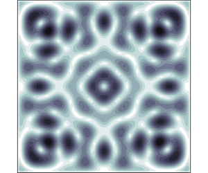Furthermore, $\text{M}_{2.18}^{-}$ is ${\mathcal{K}}$ symmetric since it has an even axial half-wavenumber, which is also easy to spot at times during the flow. Figure 11 shows the vorticity amplitudes of the three inviscid modes involved in the triadic resonance at $\unicode[STIX]{x1D714}/2\sim \unicode[STIX]{x1D70E}_{1.1}^{+}=0.3414$. The supplementary movie movie-3.avi animates the vorticity components of these modes. The modes $\text{M}_{1.1}^{+}$ and $\text{M}_{1.1}^{-}$ behave like rotating waves, one clockwise and the other counter-clockwise, but distorted by the square geometry. They have features that fill the cube; they are ‘low-order’ modes. In contrast $\text{M}_{2.18}^{-}$ has complicated $(x,y)$ structure and there is no analogy with rotating waves. The amplitude shows a very intricate $D_{4}$ symmetric pattern, but the actual mode has complicated spatio-temporal structure, with the cells lining themselves up along $x$, then $x=y$, then $y$ directions, and the cells making disparate reorientations in between. This type of behaviour is considerably more complicated than that of the modes shown in movie-1.avi and movie-2.avi.

Figure 12.

Snapshots of $\unicode[STIX]{x1D712}$ and $\unicode[STIX]{x1D709}$ in the indicated $x$ and $z$ planes at $\unicode[STIX]{x1D714}_{0}=5.8\times 10^{4}$, $\unicode[STIX]{x1D714}=0.343$ and times $t_{1}$ through $t_{4}$ corresponding to the red symbols in the time series in figure 9. The supplementary movie movie-4.avi animates these over 20 forcing periods.

Figure 12 shows snapshots of the $x$ and $z$ components of vorticity of the response flows at $\unicode[STIX]{x1D714}=5.8\times 10^{4}$ and $\unicode[STIX]{x1D714}/2=0.343$ in various $x$ and $z$ planes at the four times indicated by red symbols in the time series in figure 9. The supplementary movie movie-4.avi shows animations of these over the 20 forcing periods indicated in the time series in figure 9. Note that the axial vorticity of eigenmodes with odd axial half-wavenumbers vanishes in the midplane $z=0$, whereas for modes with even axial half-wavenumbers this component of vorticity is maximal in that plane. The animation of the axial vorticity $\unicode[STIX]{x1D709}$ in the midplane only shows behaviour that corresponds to that component of vorticity of the mode $\text{M}_{2.18}^{-}$, as shown in movie-3.avi, displaying the complicated choreography of the cells. In the plane $z=0.25$, $\unicode[STIX]{x1D709}$ of mode $\text{M}_{2.18}^{-}$ vanishes, but $\unicode[STIX]{x1D709}$ of both $\text{M}_{1.1}^{+}$ and $\text{M}_{1.1}^{-}$ is maximal. The response flow in the plane $z=0.25$ animated in movie-4.avi shows the counter-clockwise rotation of the dipole $\unicode[STIX]{x1D709}$ structure, very similar to that of $\text{M}_{1.1}^{+}$, but a little jerky with both spatial and temporal irregularities. These irregularities are primarily due to the weak influence from the clockwise rotating $\text{M}_{1.1}^{-}$ contribution. The planes $x=0$ and $x=0.25$ also show contributions from the modes involved in the triadic resonance. The rotating dipole structure from $\text{M}_{1.1}^{+}$ dominates in the $x=0.25$ plane, but in the midplane $x=0$, we are able to distinguish the contribution from $\text{M}_{2.18}^{-}$ when the symmetry plane of the dipole from $\text{M}_{1.1}^{+}$ aligns with the $x=0$ plane. Here as well, the weak contribution from $\text{M}_{1.1}^{-}$ leads to distortions. During these brief moments (such as at $t=t_{1}$ and $t_{3}$), the $n=2$ axial structure is clearly evident.

8 Discussion and conclusions

Precessional forcing of a rapidly rotating cube results in a system with spatio-temporal symmetries consisting of a reflection about the axial midplane together with a half-period translation in time, and a one quarter rotation about the axis together with a one quarter period translation in time. These symmetries, ${\mathcal{T}}_{\unicode[STIX]{x1D70F}/2}{\mathcal{K}}$ and ${\mathcal{T}}_{\unicode[STIX]{x1D70F}/4}{\mathcal{R}}_{\unicode[STIX]{x03C0}/2}$, can be combined into a purely spatial symmetry, ${\mathcal{C}}$, the centrosymmetry that is the reflection through the centre of the cube. Using direct numerical simulations of the Navier–Stokes equations with no-slip boundary conditions, we have shown that when the mean rotation rate of the cube is sufficiently fast compared to viscous dissipation processes, the primary response flows as the forcing frequency is varied can be identified as resonantly excited inviscid eigenmodes of the rotating cube, with some nominal viscous detuning. Obtaining the inviscid eigenmodes is not straightforward as the eigenmode problem is not completely separable. However, by judicious choices of the basis functions used to compute the eigenmodes, we have an efficient, accurate and robust numerical technique to compute eigenmodes with designated spatio-temporal symmetries. This has been instrumental in the detailed interpretation of the response to forcing over an extensive range of forcing frequencies. Furthermore, as viscous dissipation effects are reduced, not only are viscous detuning effects reduced and more modes with larger spatial gradients resonantly excited, but there are also triadic resonances excited. The particular spatio-temporal symmetry of the precessing cube dictates that any triadic resonance with a forced primary response flow must involve two free modes of which at least one must have a symmetry different from that of the precessing cube system. Our ability to also compute these other modes has been used to unequivocally identify the three modes involved in a triadic resonance.