1. Introduction
Among the six types of shock interference discovered by Edney (Reference Edney1968a,Reference Edneyb), type IV shock interference yields the highest aerothermal loads on a body surface. The type IV interference occurs when an oblique shock wave intersects the quasi-normal part of a strong shock wave, produced, for instance, by an incident shock wave impinging on the bow shock in front of a blunt body. A number of studies have been conducted to study the flow pattern (cf. Frame & Lewis Reference Frame and Lewis1997; Windisch, Reinartz & Müller Reference Windisch, Reinartz and Müller2016), transition between various flow patterns (cf. Bramlette Reference Bramlette1974), heat load (cf. Hains & Keyes Reference Hains and Keyes1972; Keyes & Hains Reference Keyes and Hains1973; Wieting & Holden Reference Wieting and Holden1989) and flow unsteadiness (cf. Holden et al. Reference Holden, Wieting, Moselle and Glass1988; Gaitonde & Shang Reference Gaitonde and Shang1995; Chu & Lu Reference Chu and Lu2012; Windisch et al. Reference Windisch, Reinartz and Müller2016; Khatt & Jagadeesh Reference Khatt and Jagadeesh2018). See the review of Grasso et al. (Reference Grasso, Purpura, Chanetz and Délery2003) for more related works.
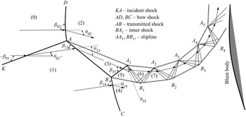
Type IV shock interference produces a jet which penetrates into the subsonic flow field downstream of the bow shock. A typical structure of type IV shock interference where the jet is supersonic is displayed in figure 1. The first portion of the jet is bounded by the transmitted shock  $AB$ that connects the first and second triple points
 $A$ and
 $B$, the inner shock
 $BA_{1}$ and the slipline
 $AA_{1}$. The second portion of the jet is downstream of the inner shock. When this jet touches the body, it produces high stagnation heating (Wieting & Holden Reference Wieting and Holden1989). When the incident shock wave takes a high position, the jet may bend upward without stagnating on the body and the jet is called type IVa or type VII shock interference (Yamamoto, Takasu & Nagatomo Reference Yamamoto, Takasu and Nagatomo1999; Boldyrev et al. Reference Boldyrev, Borovoy, Chinilov, Gusev, Krutiy, Struminskaya, Yakovleva, Délery and Chanetz2001; Windisch et al. Reference Windisch, Reinartz and Müller2016).
Schematic display of supersonic jet in type IV shock interference.

The second portion downstream of the inner shock contains a series of expansion and compression waves reflecting between the two sliplines, to satisfy the pressure continuity condition which states that, across a slipline, the pressure is continuous and in the subsonic flow regions outside the jet the pressure is continuous. If an expansion/compression wave follows a compression/expansion wave when the latter touches the slipline, then it is obvious that the pressure continuity condition is satisfied. In a real situation the compression waves may be composed of Mach waves, which finally focus to form a shock wave before touching the slipline, and the exact form of the compression waves may be problem dependent. Thus, there is some uncertainty in the representation of these compression waves. For instance, Edney used a shock wave to represent each compression wave (Reference Edney1968b, figure 13). Grasso et al. (Reference Grasso, Purpura, Chanetz and Délery2003, figure 2) used a series of non-focusing Mach waves to represent each compression wave. In figure 1, the sketched compression waves after the inner shock  $BA_{1}$ focus exactly on points
 $A_{2},A_{3},A_{4}$ and
 $A_{5}$ just for ease of comprehension.
Since the inner shock ( $BA_{1}$) as shown in figure 1 may be regarded as the reflected shock of the second triple point
 $B$ and since there exists a region of flow parameters in which the reflected shock of a general triple shock structure is a strong one (Chow & Chang Reference Chow and Chang1974), the jet may be transonic, i.e. the flow is supersonic ahead of the inner shock and subsonic downstream of this inner shock. A transonic jet is indeed observed by Guan et al. (Reference Guan, Bai, Lin and Wu2020). However, the condition to have transonic jet and the flow pattern inside the transonic jet have not been considered previously and these issues will be considered in this paper within the context of steady and inviscid flow.
In § 2, with some details given in Appendix A, the critical conditions for a transonic jet (as well as supersonic and subsonic) will be derived and numerical evidence of a transonic jet using computational fluid dynamics (CFD) will be provided.
Due to the pressure gradient outside the jet and due to pressure continuity across the slipline  $AA_{1}$, compression waves will be developed in the first portion of the jet (ahead of the inner shock). In § 3, we will show that these compression waves reshape the shocks
 $AB$ and
 $BA_{1}$ and advance the transition from supersonic jet to transonic jet.
For a supersonic jet, as shown in figure 1, the alternative appearance of compression and expansion waves follows from the condition of pressure continuity across the sliplines (Edney Reference Edney1968b). In § 2.4 we will show that, for a transonic jet, the jet has a two-branch structure: the upper branch is like a supersonic jet and the lower branch is subsonic. This two-branch jet is a new type of jet never observed before (to the knowledge of the authors) so we attempt to explain in § 4 and Appendix B how it is produced. We explain that the two-branch structure is an outcome of the pressure continuity condition across the slipline: the inner shock is weakened by the preceding compression waves and the downstream disturbance to have a sonic end that creates a sonic line emanating from  $A_{1}$, and this sonic flow is able to accelerate to drop the pressure further through creating an expansion fan, making the pressure continuous across the slipline near
 $A_{1}$.
2. Critical condition for a transonic jet
In this section, we provide the definition and shock theory used in our analysis (including the triple point theory of von Neumann Reference von Neumann1945), derive the critical conditions for a transonic jet and show numerical evidence of a transonic jet.
2.1. Definition and shock theory
The type of jets for type IV shock interaction is here studied using flow properties in the vicinity of triple points  $A$ and
 $B$, as shown in figure 1. In this section, the flow is considered uniform in regions
 $(3)$ and
 $(5)$ and we use subscript
 $k$ to denote the flow parameters in region
 $(k)$. For instance, the Mach number in region
 $(3)$ is denoted
 $M_{3}$.
The jet is said to be supersonic if  $M_{3}>1$ and
 $M_{5}>1$, transonic if
 $M_{3}>1$ and
 $M_{5}<1$ (if the jet exists), and subsonic if
 $M_{3}<1$ (in this case, shock
 $BA_{1}$ and the downstream wave fans do not exist). However, the transonic jet case is much more complex than this. As will be shown in § 2.3, for the case with
 $M_{3}>1$ and
 $M_{5}<1$, there are conditions where the second triple point
 $B$ does not exist, which means that there is no jet in the usual sense. In § 3, we will see that compression waves developed inside the triangle
 $ABA_{1}$ due to the pressure gradient above the slipline
 $AA_{1}$ will make the flow non-uniform inside the triangle and alter the transition conditions. Furthermore, we will see in §§ 3 and 4 that, in the case of a transonic jet, the region
 $(5)$ will be hybrid supersonic–subsonic, instead of being purely subsonic.
Here, in this section, the transition condition from a subsonic to a transonic jet is determined by the sonic condition  $M_{3}=1$ and the transition condition from a transonic to a supersonic jet is determined by the sonic condition
 $M_{5}=1$. These two conditions, if they exist, enclose the domain for the existence of a transonic jet.
Although we will display results with a high enough Mach number, in this paper, we do not consider real gas effect. Thus, we will use the classical shock relations for a perfect gas in the analysis. Now, let us recall some classical shock expressions needed in the present paper.
If we use subscripts  $u$ and
 $d$ to denote the flow status in regions upstream and downstream of a shock wave, then the shock angle
 $\beta _{ud}$ (shock slope angle with respect to the upstream flow direction) is related to the flow deflection angle
 $\theta _{ud}$ (angle change of flow direction across the shock) by the shock angle relation
 $\tan \theta _{ud}=\,f_{\theta }(M_{u} ,\beta _{ud})$ and the Mach number and pressure satisfies
 $M_{d}=\,f_{M} (M_{u},\beta _{d})$ and
 $p_{d}=p_{u}\,f_{p}(M_{u},\beta _{ud})$, with
 \begin{equation} \left\{\begin{array}{@{}l}
f_{\theta}({M,\beta})=\dfrac{2\left(
{M}^{2}{\sin}^{2}{\beta}-1\right) }{\left( {M}^{2}\left(
\gamma+\cos{2\beta}\right) +2\right) \tan{\beta}}\\
f_{M}(M,{\beta})=\sqrt{\dfrac{\left( \gamma-1\right)
{M}^{2}+2}{2\gamma {M}^{2}{\sin}^{2}{\beta}-\left(
\gamma-1\right) }+\dfrac{2{M}^{2}{\cos} ^{2}{\beta}}{\left(
\gamma-1\right) {M}^{2}{\sin}^{2}{\beta}+2}}\\
f_{p}(M,{\beta})=1+\dfrac{2\gamma}{\gamma+1}\left(
{M}^{2}{\sin}^{2}{\beta }-1\right),
\end{array}\right. \end{equation}
where  $\gamma$ is the ratio of specific heats.
Let  ${\beta }_{m}$ be the shock angle at the detachment condition (shock slope angle that corresponds to maximum flow deflection angle at given Mach number), i.e. at
 ${\beta }$ with
 ${{\rm d}\,f_{\theta }}/{{\rm d}{\beta }}=0$ (which occurs at the detachment angle). Using the expression in (2.1) for
 $f_{\theta }(M,{\beta })$, one has
 \begin{equation} \sin^{2}{\beta}_{m}=\frac{1}{\gamma M^{2}}\left( \frac{\gamma+1}{4} M^{2}-1+\sqrt{(\gamma+1)\left(1+\frac{\gamma-1}{2}M^{2}+\frac{\gamma+1}{16}M^{4} \right)}\right). \end{equation}
A downstream sonic flow occurs at  $\beta =\beta _{M_{d}=1}$ where
 $\beta _{M_{d}=1}$ is the shock angle at which
 $f_{M}(M,{\beta }_{M_{d}=1} )=1$. Using the expression in (2.1) for
 $f_{M}(M,{\beta }_{M_{d}=1}{)}$, one has
 \begin{equation} \frac{\left( \gamma-1\right) {M}^{2}+2}{2\gamma{M}^{2}{\sin}^{2}{\beta }_{M_{d}=1}-\left( \gamma-1\right) }+\frac{2{M}^{2}{\cos}^{2}{\beta} _{M_{d}=1}}{\left( \gamma-1\right) {M}^{2}{\sin}^{2}{\beta}_{M_{d}=1}+2}=1 . \end{equation}
From the classical theory for oblique shock waves (cf. Anderson Reference Anderson2001, p. 315), we know that: (i) the shock solution admits  ${\beta <\beta }_{m}$ (for which the shock is said to belong to the weak solution) and
 ${\beta >\beta }_{m}$ (for which the shock is said to belong to the strong solution) and (ii) for given
 $\theta$ and upstream
 $M$, one has
 ${\beta }_{M_{d}=1}<\beta _{m}$, (iii) for
 ${\beta <\beta }_{M_{d}=1}$, the downstream flow of the shock is supersonic (the shock is then called a weak shock wave) and for
 ${\beta >\beta }_{M_{d}=1}$ the downstream flow is subsonic (the shock is now called a strong shock).
The analysis for finding the critical conditions relies on the use of the well-known triple point theory due to von Neumann (Reference von Neumann1943, Reference von Neumann1945), which describes the relationship between flow quantities in various regions in the vicinity of a triple point (typical structure of type IV shock interaction).
Consider triple point theory applied to point  $A$. The flow parameters in region
 $(0)$ are given, the shock angle
 ${{\beta _{0{1}}}}$ or the flow deflection
 ${\theta _{01}}$ connected to
 ${{\beta _{0{1}}}}$ by
 $\tan {\theta _{01}}={\,f_{\theta }}( {{M_{0}},{\beta _{0{1}}}})$, is also given. First, the Mach number and pressure in region
 $(1)$ are obtained from
 $M_{1}=\,f_{M}(M_{0},\beta _{01})$ and
 $p_{1}=p_{0}\,f_{p}(M_{0},\beta _{01})$. Then the pressure
 $p_{2}$ is obtained from
 $p_{2}=p_{0}\,f_{p}(M_{0},\beta _{02})$ for shock
 $AD$ and the pressure
 $p_{3}$ is obtained from
 $p_{3}=p_{1}\,f_{p} (M_{1},\beta _{13})$ for shock
 $AB$. The shock angle
 $\beta _{13}$ is solved from
 $\tan {\theta _{13}}=\,{f_{\theta }}( {{M_{1}},{\beta _{{13}}}})$ for the weak solution and
 $\beta _{02}$ is solved from
 $\tan {\theta _{02} }=\,{f_{\theta }}( {{M_{0}},{\beta _{{02}}}})$ for the strong solution. Here, the flow deflection angles
 ${\theta _{13}}$ and
 ${\theta _{02}}$ are obtained from the flow parallel conditions
 $\theta _{02}=\theta _{AA_{1}}$ and
 $\theta _{13}=\theta _{01}-\theta _{AA_{1}}$, where
 $\theta _{AA_{1}}$ is the slipline angle of
 $AA_{1}$ and is obtained by using the pressure balance condition
 $p_{2}=p_{3}$.
The triple point theory applied to point  $B$ is similar to that for triple point
 $A$.
2.2. Conditions for a transonic jet
Here, we provide two conditions: one condition, denoted  $\theta _{01} =\theta _{sub}^{tran}(M_{0})$, corresponds to
 $M_{3}=1$, and the other, denoted
 $\theta _{01}=\theta _{sup}^{tran}(M_{0})$, corresponds to
 $M_{5}=1$.
The condition  $\theta _{01}=\theta _{sub}^{tran}(M_{0})$ is the necessary critical condition for transition from a subsonic jet to a transonic jet. The reason it is a necessary condition is that, when this condition is met, one may still have no transonic jet, as discussed in § 2.3, where we provide another critical condition. The condition
 $\theta _{01}=\theta _{sup }^{tran}(M_{0})$ is the critical condition for transition from a supersonic jet to a transonic jet. The detailed expressions to obtain these critical conditions will be given in Appendix A. Below, we just summarize the main steps to obtain them, before giving the critical conditions in the plane
 $M_{0}\text {--}{\theta _{01}}$.
The necessary condition for transition from a subsonic to a transonic jet corresponds to the sonic condition  $M_{3}=1$. First, we solve the triple point theory for the triple point
 $A$ (see § 2.1) to get the shock angle
 $\beta _{13}$ for a given
 ${M}_{0}$ and
 ${\theta _{01}}$. The Mach number
 $M_{3}$ in region
 $(3)$ is then obtained by
 $M_{3}=\,f_{M}(M_{1},\beta _{13})$. For a given inflow Mach
 $M_{0}$, we search a flow deflection angle
 $\theta _{01}=\theta _{sub}^{tran}(M_{0})$ for which the sonic condition
 $M_{3}=1$ holds.
The transition condition from a supersonic to a transonic jet corresponds to the sonic condition  $M_{5}=1$ (for
 $M_{3}>1$). First, we solve the triple point theory for point
 $A$. Now, the shock
 $AB$, with its shock angle
 $\beta _{13}$ and its upstream Mach number
 $M_{1}$, already known from the triple point solution of point
 $A$, is considered as the incident shock wave for triple point
 $B$. The triple point solution of point
 $B$, if it exists, then gives the solution
 $M_{5}$. For a given inflow Mach number
 $M_{0}$, we search for a flow deflection angle
 $\theta _{01}=\theta _{sup}^{tran}(M_{0})$ for which the sonic condition
 $M_{5}=1$ holds.
The critical conditions  ${\theta _{01}=\theta }_{sub}^{tran}(M_{0})$ and
 $\theta _{01}=\theta _{sup}^{tran}(M_{0})$ in the plane
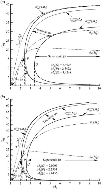
 $M_{0}\text {--}{\theta _{01}}$ thus obtained are shown in figure 2(a) for
 $\gamma =1.4$ and in figure 2(b) for
 $\gamma =1.1$. For cold air we have
 $\gamma =1.4$. The reason we display the results for
 $\gamma =1.1$ is to show that the transition conditions also depend on the ratio of specific heats, although the result with a smaller value
 $\gamma =1.1$ may partly account for the high temperature effect of high Mach number flow since such an effect equivalently reduces
 $\gamma$.
Transition criteria in the  $M_{0}-\theta _{01}$ plan; (a)
 $\gamma =1.4$, (b)
 $\gamma =1.1$.

In figure 2, we also display the condition  $\theta _{01} =\theta _{max}(M_{0})$ for the incident shock wave to detach, the detachment condition
 $\theta _{01}=\theta _{D}(M_{0})$ for Mach reflection of the triple point
 $A$ and the von Neumann condition
 $\theta _{01}=\theta _{N}(M_{0})$ for Mach reflection of triple point
 $A$.
For  $\gamma =1.4$, the two curves
 $\theta _{01}={\theta }_{sub}^{tran}(M_{0} )$ and
 $\theta _{01}=\theta _{sup}^{tran}(M_{0})$ enclose the region inside which the jet is transonic if the second triple point exists, i.e. the first part of the jet (triangle
 $ABA_{1}$) is supersonic while the rest (downstream of
 $BA_{1}$) is (theoretically) subsonic. The critical curve
 $\theta _{01}=\theta _{sup}^{tran}(M_{0})$ encloses a region where the jet is purely supersonic. Outside of the critical curve
 $\theta _{01}=\theta _{sub}^{tran}(M_{0})$ the jet is purely subsonic (if a jet exists in this case).
We observe that both  $\theta _{01}={\theta }_{sub}^{tran}(M_{0})$ and
 $\theta _{01}=\theta _{sup}^{tran}(M_{0})$ have a (near) C-shape in the
 $M_{0}\text {--}\theta _{01}$ plane. The left-most point
 $O$ of
 $\theta _{01}={\theta }_{sub}^{tran}(M_{0})$ lies at
 $M_{0}\approx 2.4$ and the left-most point
 $Q$ of
 $\theta _{01}=\theta _{sup}^{tran}(M_{0})$ lies at
 $M_{0} \approx 3.4$.
The transition curves for  $\gamma =1.1$ are similar to that for
 $\gamma =1.4$, apart from the fact that the two curves
 $\theta _{01}={\theta }_{sub}^{tran}(M_{0})$ and
 $\theta _{01}=\theta _{sup}^{tran}(M_{0})$ move some distance to the left. In the rest of the paper we only consider air with
 $\gamma =1.4$.
The curve  $\theta _{01}={\theta }_{nojet}^{tran}(M_{0})$ shown in figure 2 is the critical condition to have no jet and will be discussed in § 2.3.
Now, we display the shock polars for two conditions:  $M_{0}=2.426$,
 $\theta _{01}=13^{\circ }$ and
 $M_{0}=3.435,\theta _{01}=13^{\circ }$, which lie on the critical transition lines
 $\theta _{01}={\theta }_{sub}^{tran}(M_{0})$ and
 $\theta _{01}={\theta }_{sup}^{tran}(M_{0})$, according to figure 2. Following Kawamura & Saito (Reference Kawamura and Saito1956), we use
 $\varGamma (k)$ to denote the shock polar along which is the locus of all the flow states that could be obtained from any shock wave with a fixed upstream state
 $(k)$. The sonic point will be marked with an open circle. The shock polars are displayed in figure 3. When
 $M_{0}=2.426$,
 $\theta _{01}=13^{\circ }$, there is only one triple point and the polar
 $\varGamma (0)$ intersects the polar
 $\varGamma (1)$ exactly at its sonic point (figure 3a). In this case, we have
 $M_{3}=1$, i.e.
 $\theta _{01}={\theta }_{sub}^{tran}(M_{0})$. When
 $M_{0}=3.435$,
 $\theta _{01}=13^{\circ }$, the polar
 $\varGamma (1)$ intersects the polar
 $\varGamma (3)$ exactly at its sonic point (figure 3b). In this case, we have
 $M_{5}=1$, i.e.
 $\theta _{01}={\theta }_{sup}^{tran}(M _{0})$.
Shock polars for  $\theta _{01}=13^{\circ }$. (a) On the critical line
 $\theta _{sub}^{tran}$ with
 $M_{0}=2.426$. (b) On the critical line
 $\theta _{sup}^{tran}$ with
 $M_{0}=3.435$.

2.3. Condition of no jet and region with a transonic jet
As mentioned in § 2.1, for the case with  $M_{3}>1$ and
 $M_{5}<1$, there are conditions where the second triple point
 $B$ does not exist, which means that there is no jet in the usual sense. This occurs when the polar
 $\varGamma (3)$ lies completely inside of
 $\varGamma (1)$, as displayed in figure 4(a) for
 $M_{0}=2.5$,
 $\theta _{01}=13^{\circ }$. Appendix A.3 used the theory of Chernyshov, Kapralova & Savelova (Reference Chernyshov, Kapralova and Savelova2021) to derive the condition
 $\theta _{01}={\theta }_{nojet}^{tran}(M_{0})$, beyond which the second triple point
 $B$ and the jet do not exist. The critical condition
 $\theta _{01}={\theta }_{nojet}^{tran}(M_{0})$ corresponds to the polar
 $\varGamma (3)$ tangent to
 $\varGamma (1)$, as shown in figure 4(b) for
 $M_{0}=2.548,$
 $\theta _{01}=13^{\circ }$.
Shock polars for  $\theta _{01}=13^{\circ }$. (a) Between the critical lines
 $\theta _{sub}^{tran}$ and
 $\theta _{nojet}^{tran}$ (
 $M_{0}=2.5$). (b) On the critical line
 $\theta _{nojet}^{tran}$ (
 $M_{0}=2.548$).

The curve  $\theta _{01}={\theta }_{nojet}^{tran}(M_{0}{)}$ is also displayed in figure 2(a,b). For
 $\gamma =1.4$, its left-most point
 $P$ has
 $M_{0}\approx 2.5422$. The curve
 $\theta _{01}={\theta }_{nojet}^{tran} (M_{0}{)}$ lies between
 $\theta _{01}={\theta }_{sub}^{tran}(M_{0}{)}$ (necessary condition) and
 $\theta _{01}={\theta }_{sup}^{tran}(M_{0}{)}$. In the region between
 $\theta _{01}={\theta }_{sub}^{tran}(M_{0}{)}$ and
 $\theta _{01}={\theta }_{nojet}^{tran}(M_{0}{)}$, the flow downstream of
 $AB$ is still supersonic but the second triple point
 $B$ does not exist.
In conclusion, a transonic jet occurs in the region bounded by the critical conditions  $\theta _{01}={\theta }_{nojet}^{tran}(M_{0}{)}$ and
 $\theta _{01}=\theta _{sup}^{tran}(M_{0}{)}$, which are shown in figure 2(a,b).
In the present paper, we focus on the case with a transonic jet, so in the following we only consider the region enclosed by  $\theta _{01}=\theta _{nojet}^{tran}(M_{0})$ and
 $\theta _{01}={\theta }_{sup}^{tran}(M _{0})$.
2.4. Numerical evidence of a transonic jet and observation of a two-branch transonic jet
CFD is used to obtain numerical solutions. The inviscid compressible Euler equations for a perfect gas with a ratio of specific heat  $\gamma =1.4$ are solved numerically using the second-order Roe scheme (Roe Reference Roe1986) on a structured grid with
 $500\times 800$ points. The grid is refined in the jet and there are approximately
 $50$ grid points in the direction perpendicular to the jet. The grid has been chosen such that the flow structure no longer changes and the accuracy is checked using the Edney (Reference Edney1968b) experimental measurement for
 $M_{0}=4.6$ and
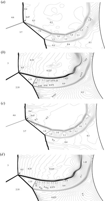
 $\theta _{01}=10^{\circ }$. According to the transition criterion as shown in figure 2(a), the jet should be supersonic. The computed Mach contours shown in figure 5(a) agree well with figure 13 of Edney (Reference Edney1968b).
Mach contours at two instants for two set of conditions. (a) Supersonic jet at  $\bar {t}=115$ with
 $M_{0}=4.6$,
 $\theta _{01}=10^{\circ }$, (b) transonic jet at
 $\bar {t}=52$ with
 $M_{0}=3$ and
 $\theta _{01}=13^{\circ }$, (c) supersonic jet at another instant
 $\bar {t}=120$ and (d) transonic jet at
 $\bar {t}=62$. The time
 $\bar {t}$ is normalized by the reference time (radius of the blunt body divided by the free-stream velocity).

Now we select the typical point  $M_{0}=3$ and
 $\theta _{01}=13^{\circ }$ inside the transonic jet region of figure 2(a). According to the numerical result shown in figure 5(b), the jet downstream of the inner shock indeed has a subsonic region. However, the jet is not purely subsonic but displays a two-branch structure: the upper one is supersonic while the lower one is subsonic. This unusual phenomenon will be considered in § 4. Note that the present numerical result is for inviscid flow and, due to the sharp gradients in the jet, viscous effects in real flow could very well make the noted two-branch structure more difficult to obtain or detect. In future work the viscous effect on the two-branch structure may be considered. We also note that the entropy is continuous across the interface between the two branches.
We have also computed the flow for  $M_{0}=2$ and
 $\theta _{01}=13^{\circ }$, which should have a subsonic jet according to the transition criterion, as shown in figure 2(a). According to our numerical results, not shown here, there is only one triple point and one slipline.
The type IV interaction is known to display unsteadiness (cf. Holden et al. Reference Holden, Wieting, Moselle and Glass1988; Gaitonde & Shang Reference Gaitonde and Shang1995; Chu & Lu Reference Chu and Lu2012; Windisch et al. Reference Windisch, Reinartz and Müller2016; Khatt & Jagadeesh Reference Khatt and Jagadeesh2018). The numerical method used has a second-order time accuracy and the flow is unsteady. The Mach contours displayed in figures 5(a) and 5(b) correspond to some instant after a long time of iteration. As shown in figures 5(c) and 5(d), the local flow parameters at other instants have minor changes compared with those shown in figures 5(a) and 5(b), showing unsteadiness. However, the observed overall flow configuration, of interest in this paper, does not change with time.
Note that Lu et al. (Reference Lu, Yue, Xiao and Zhang2013) studied the interaction between isentropic compression waves and a bow shock and noted for some condition a transonic jet in their numerical results. The exact flow pattern for their transonic jet and the transition conditions to have their transonic jet may deserve a separate study.
3. Compression waves and advance of transition
In this section, we first consider the role of the compression waves due to the streamwise pressure gradient in the subsonic region above the slipline  $AA_{1}$ in the shape of the transmitted shock
 $AB$ and inner shock
 $BA_{1}$, we then show that this role will advance the transition from a supersonic jet to a transonic jet.
3.1. Compression waves in the triangle  $ABA_{1}$

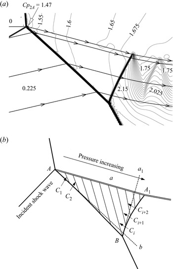
Figure 6(a) displays, for the transonic jet case with  $M_{0}=3$ and
 $\theta _{01}=13^{\circ }$, the pressure contours in terms of the pressure coefficient. It is clear that, above the slipline
 $AA_{1}$, there is a positive pressure gradient. The pressure just above the slipline
 $AA_{1}$ will be denoted by
 $p_{slip}$. Positive pressure gradient here means
 ${\rm d}p_{slip}/{\rm d}s>0$, where
 $s$ is the distance measured along the slipline
 $AA_{1}$.
Flow pattern for  $M_{0}=3$ and
 $\theta _{01}=13^{\circ }$. (a) Pressure contours showing positive pressure gradient above
 $AA_{1}$. (b) Illustration of compression waves
 $C_{1},C_{2},\ldots$. The lines
 $Ab$ and
 $Ba_{1}$ are straight lines tangent to the shocks
 $AB$ and
 $BA_{1}$ at point
 $A$ and
 $B$, respectively.

Now we provide a simplified model of compression waves. Since the pressure is continuous across the slipline  $AA_{1}$, the flow inside the triangle
 $ABA_{1}$ also has a positive pressure gradient and this pressure gradient generates a series of compression waves
 $C_{1},C_{2},\ldots$ that propagate in the way illustrated in figure 6(b). To account for the influence of these compression waves, we simply assume the flow is isentropic and irrotational inside the triangle
 $ABA_{1}$, so we represent the compression waves by straight characteristic lines of the second family satisfying
 ${{\rm d} y}/{{\rm d} x}=\tan (\theta +\mu )$, where
 $\mu$ is the Mach angle. Along each characteristic line the pressure is assumed to be constant, i.e.
 $p=p_{slip}$ (this appears to be so according to figure 6a). The possible reflected waves of
 $C_{1},C_{2},\ldots$ from
 $AB$ is not considered.
Under the above simplification, the variation  ${\rm d}\theta$ of the flow deflection angle across the compression waves can be related to the pressure variation
 ${\rm d}p={\rm d}p_{slip}$ and the Mach number variation
 ${\rm d}M$ through the Mach wave relations
 $$\begin{gather} {\rm d}p_{slip}=\varPhi(M,p)\,{\rm d}\theta,\quad \varPhi(M,p)=\frac{\gamma Mp}{\sqrt{M^{2}-1}}, \end{gather}$$
 $$\begin{gather}{\rm d}M=\varPsi(M,p)\,{\rm d}\theta,\quad \varPsi(M,p)={-}\frac{M}{\sqrt{M^{2}-1}}\left( 1+\frac{\gamma-1}{2}M^{2}\right) . \end{gather}$$
Due to compression waves, the flow is non-uniform in regions  $(3)$ and
 $(5)$. Thus,
 $M_{3}^{(B)}$, which denotes the Mach number in region
 $(3)$ and in the vicinity of point
 $B$, is different to
 $M_{3}^{(A)}$, which denotes the Mach number in region
 $(3)$ but in the vicinity of point
 $A$. To further simplify the analysis, we assume the compression waves are weak enough so that the variation of parameters inside the triangle
 $ABA_{1}$ is small. Under this assumption, the coefficients
 $\varPhi (M,p)$ and
 $\varPsi (M,p)$ in (3.1a,b) and (3.2a,b) and those in similar formulas given below will be evaluated using the uniform solutions
 $M_{3}$,
 $p_{3}$,
 ${\beta }_{13}$ and
 ${\beta } _{35}$ given in § 2. For instance, we will simply put
 $\varPhi (M,p)=\varPhi (M_{3},p_{3})$ and
 $\varPsi (M,p)=\varPsi (M_{3},p_{3})$. The expressions (3.1a,b) and (3.2a,b) can then be used to give a relation between
 $dM$ and
 $dp$ (across the compression waves)
 \begin{equation} \frac{{\rm d}M}{{\rm d}p_{slip}}={-}\left( 1+\frac{\gamma-1}{2}M_{3}^{2}\right) \frac {1}{\gamma p_{3}} . \end{equation}
Below, we will use the Mach wave relations (3.1a,b), (3.2a,b) and (3.3) to account for the influence of compression waves on the deflection of transmitted shock  $AB$ from a straight line (similar effect by compression waves on the inner shock
 $BA_{1}$ will be considered in § 4). Note that, the interaction between Mach waves and shock waves has been considered for various other purposes (Moeckel Reference Moeckel1952; Rosciszewski Reference Rosciszewski1960; Hasimoto Reference Hasimoto1964; Li & Ben-Dor Reference Li and Ben-Dor1995; Meshkov, Omelchenko & Uskov Reference Meshkov, Omelchenko and Uskov2002; Silnikov, Chernyshov & Uskov Reference Silnikov, Chernyshov and Uskov2014; Uskov & Chernyshov Reference Uskov and Chernyshov2014).
3.2. Advance of transition from a supersonic jet to a transonic jet
Now we consider the role of compression waves  $C_{1},C_{2},\ldots,C_{i}$ in the shape of transmitted shock
 $AB$ as well as on the advance of transition from a supersonic jet to a transonic jet. For this purpose, we rewrite the shock angle relation as
 $\theta =F(M,{\beta })$ with
 $F(M,{\beta })=\arctan \,f_{\theta }({M,\beta })$, where
 $f_{\theta }({M,\beta })$ is defined in (2.1).
The Mach number  $M_{1}$ upstream of shock
 $AB$ is constant so that differentiating
 $\theta =F(M,{\beta })$ gives
 \begin{equation} \frac{{\rm d}{\beta}}{{\rm d}\theta}=\frac{1}{G(M_{1},{\beta}_{13})},\quad G(M,{\beta })=\frac{\partial F(M,{\beta})}{\partial{\beta}}.\end{equation}
Combining shock angle relation (3.4a,b) and the Mach wave relation (3.1a,b) then gives the following relation between the shock angle of  $AB$ and the pressure gradient
 ${\rm d}p_{slip}$ along the slipline
 $Aa$:
 \begin{equation} \frac{{\rm d}{\beta}}{{\rm d}p_{slip}}=\frac{\sqrt{M_{3}^{2}-1}}{\gamma M_{3}p_{3} G(M_{1},{\beta}_{13})}. \end{equation}
One can check that, for a weak shock  $AB$, we have
 ${{\rm d}{\beta }}/{{\rm d}p_{slip} }>0$, thus the shock
 $AB$ deflects from a straight line toward the lower side as shown in figure 6(b) and, at the triple point
 $B$, the shock angle
 ${\beta }_{13}^{(B)}$ is larger than
 ${\beta }_{13}$ (shock angle in case of no compression waves). Integrating (3.5) from point
 $A$ to point
 $B$ gives
 \begin{equation} {\beta}_{13}^{(B)}={\beta}_{13}+\frac{\sqrt{M_{3}^{2}-1}}{\gamma M_{3} p_{3}G(M_{1},{\beta}_{13})}(p_{slip}^{(a)}-p_{3}) , \end{equation}
where  $p_{slip}^{(a)}$ is the pressure at point
 $a$ (this point is connected to
 $B$ by a characteristic line). There is no simple theory to provide the pressure
 $p_{slip}^{(a)}$ in this paper. Below, we simply use CFD data for
 $p_{slip}^{(a)}$ once it is needed in analysis. After
 ${\beta }_{13}^{(B)}$ is thus obtained, the shock angle relation
 $\theta _{13}^{(B)}=F(M_{1},{\beta }_{13}^{(B)})$ is used to evaluate
 $\theta _{13}^{(B)}$.
Now we discuss how the transition condition  $\theta _{01}=\theta _{sup} ^{tran}(M_{0}{)}$ is modified by the compression waves. The expression (3.6) provides an approximate evaluation of the shock angle
 ${\beta }_{13}^{(B)}$ of
 $AB$ near the triple point
 $B$ when the role of compression waves
 $C_{1},C_{2},\ldots,C_{i}$ is accounted for. The triple point theory at point
 $B$ using this updated shock angle
 ${\beta }_{13}^{(B)}$ for the incident shock wave
 $AB$ gives an updated value of
 $M_{5}$, now denoted
 $M_{5}^{(B)}$. In the modified transition criterion, it is this updated
 $M_{5}^{(B)}$ which is used to define the jet type: if
 $M_{5}^{(B)}>1$, the jet is supersonic and if
 $M_{5}^{(B)}<1$, the jet is transonic. Since
 ${\beta }_{13}^{(B)} >{\beta }_{13}$, thus
 $M_{5}^{(B)}$ is smaller than
 $M_{5}$. Table 1 gives, for four conditions, the jet types predicted using the original criterion (shown in figure 2a), the modified transition criterion and CFD observation. For Case 2, while the original theory predicts a supersonic jet, both the modified criterion and CFD show a transonic jet. Case 3 is close to the modified transition criterion, i.e. for
 $\theta _{01}=13^{\circ }$, the modified transition occurs at
 $M_{0}\approx 3.7$, while the original transition criterion corresponds to
 $M_{0}\approx 3.42$. Thus, compression waves developed due to the pressure gradient
 ${\rm d}p_{slip}/{\rm d}s>0$ advance transition from a supersonic jet to a transonic jet.
Predicted and observed types of the jet cases for  $\theta _{01}=13^{\circ }$ and various Mach numbers.

4. Two-branch structure of the transonic jet
In this section, we consider how the two-branch structure of the transonic jet, for which the upper branch is supersonic and the lower branch subsonic, as shown in figures 5(b) and 5(d), is produced. It will be shown that this two-branch structure follows from the production of a sonic line from  $BA_{1}$ downstream which the flow is able to accelerate further to become supersonic through creating an expansion fan. The sonic condition is shown to be due to the weakening of
 $BA_{1}$ by upstream disturbance (due to preceding compression waves) and downstream disturbance (which may be produced by some subtle mechanism to meet the pressure continuity requirement across the slipline).
4.1. Observation of a sonic line apparently emanating from point $A_{1}$

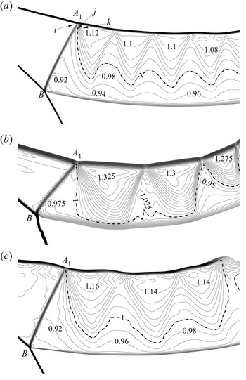
Figure 7 shows the two-branch structure of the transonic jet, for three different conditions, which are inside the transonic jet region according to table 1 or figure 2(a). For each case we observe a sonic line emanating apparently from point  $A_{1}$. Note that some parts of the sonic line in figure 7(b) touch the lower slipline, while in figures 7(a) and 7(c) the sonic line is away from the lower slipline. The solution shown in figure 7(b) is in fact near the transition condition from a transonic to a supersonic jet, so the sonic line gets closer to the lower slipline. This sonic line will be used to explain, in § 4.2, the production of the observed two-branch structure of the transonic jet.
Mach contours of the transonic jet, where the dashed line represents a sonic line with  $M=1$; (a)
 $M_{0}=3$ and
 $\theta _{01}=13^{\circ }$, (b)
 $M_{0}=3.5$ and
 $\theta _{01}=13^{\circ }$, (c)
 $M_{0}=3$ and
 $\theta _{01}=15^{\circ }$.

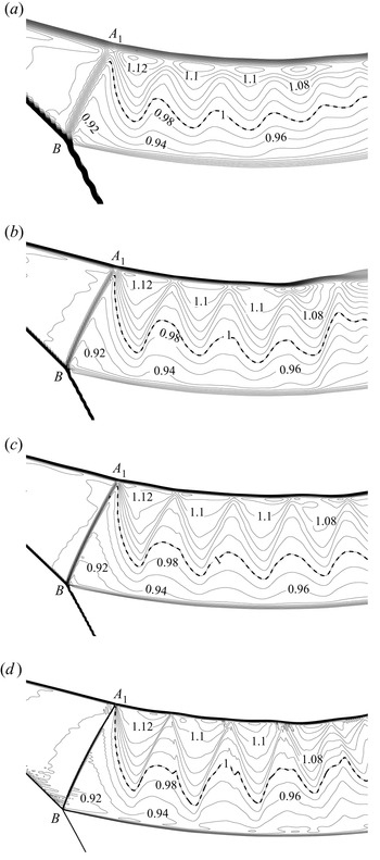
To verify that the sonic line emanates from point  $A_{1}$ and not from any inner point of the reflected shock, we perform a grid refinement study using the case shown in figure 7(a). The starting point of the sonic line indeed gets closer to point
 $A_{1}$ if the grid is further refined, as shown in figure 8(a–d) with four different grids. The number of grids is
 $9\times 10^{4}$ for grid A (approximately
 $45$ grid points along
 $BA_{1}$),
 $3.4\times 10^{5}$ for grid B (approximately
 $90$ grid points along
 $BA_{1}$),
 $1.36\times 10^{6}$ for grid C (approximately
 $180$ grid points along
 $BA_{1}$) and
 $2.08\times 10^{6}$ for grid D (approximately
 $360$ grid points along
 $BA_{1}$).
Transonic jet for  $M_{0}=3$ and
 $\theta _{01}=13^{\circ }$. (a) Grid A. (b) Grid B. (c) Grid C. (d) Grid D.

The mechanism for the creation of the sonic line at  $A_{1}$ is rather complex. According to a simplified analysis in Appendix B, it appears that the sonic line results from the weakening of
 $BA_{1}$ by the combined effect of upstream flow disturbance (due to the preceding compression waves) and downstream flow disturbance (due to local flow stream deflection near
 $A_{1}$ and this deflection follows from the pressure continuity requirement across the slipline).
4.2. Postulated mechanism by which the two-branch transonic jet structure is produced
Now we postulate the mechanism for the production of two-branch transonic jet, based on the observation of a sonic line emanating from point  $A_{1}$ and using the schematic displayed in figure 9 of the wave pattern in the vicinity of the inner shock
 $BA_{1}$. Figure 9 is sketched following the numerical solution shown in figure 7(a).
Schematic display of the wave pattern in the vicinity of the inner shock  $BA_{1}$.

First, it is physically impossible that, for a transonic jet, the flow behind the inner shock is subsonic everywhere. In fact, the pressure continuity condition, similar to that stated in the Introduction for a supersonic jet, is violated if the flow downstream of the inner shock is subsonic everywhere. To see this, let us consider the three points  $i$,
 $j$ and
 $k$ as shown in figure 9. If a pure subsonic flow is assumed in all regions downstream of
 $BA_{1}$, then the expansion fan between points
 $j$ and
 $k$ does not exist. In this case,
 $p_{k}=p_{j}>p_{i}$, which is impossible since, due to pressure continuity across a slipline, the pressures at points
 $i,j,k$ should be balanced by the pressure in the subsonic region
 $(0)$ above the slipline
 $AA_{1}$, and the inequality
 $p_{k}=p_{j}>p_{i}$ means pressure discontinuity in the subsonic region
 $(0)$, which is impossible since pressure discontinuity cannot be sustained by a subsonic flow.
As we have shown in § 4.1, at point  $j$, the flow should be sonic, i.e.
 $M_{5}^{(A_{1})}=1$. A sonic flow at point
 $j$ is able to accelerate to supersonic flow at point
 $k$ through generating an expansion fan, as displayed in figure 9. Due to this expansion fan the pressure continuity condition (
 $p_{k}=p_{i}$) is met as in case of a pure supersonic jet. The reason that the flow is not supersonic at
 $j$ would be that the condition
 $M_{5}^{(A_{1})}=1$ corresponds to the least effort required by the compressive waves ahead of
 $BA_{1}$ to weaken
 $BA_{1}$ to allow for pressure continuity.
Finally, through generating both disturbances upstream and downstream of  $BA_{1}$, the pressure gradient outside the slipline appears to play the essential role to weaken
 $BA_{1}$ until the downstream flow has a sonic line emanating from
 $A_{1}$. A last question is whether the pressure gradient is large enough to sustain such a structure. Since the flow describing the shock
 $BA_{1}$ depends on the pressure gradient outside of the upper slipline (see Appendix B), the Mach number
 $M_{5}^{(A_{1})}$ should depend on
 $p_{slip}^{(A_{1})}$ (pressure at point
 $A_{1}$) and
 $p_{slip}^{(a)}$ (pressure at point
 $a$ as shown in 6a). Let the functional form of
 $M_{5}^{(A_{1})}$ be
 $M_{5}^{(A_{1})}=\,F_{1}(M_{3}^{(B)},{\beta }_{35} ^{(B)},\bar {p}_{slip}^{(A_{1})},\bar {p}_{slip}^{(a)})$, where
 $\bar {p}_{slip}^{(a)}=p_{slip}^{(a)}/p_{3}$ and
 $\bar {p} _{slip}^{(A_{1})}=p_{slip}^{(A_{1})}/p_{3}$. The sonic line assumption
 $M_{5}^{(A_{1})}=1$ then gives the pressure constraint
 \begin{equation} F_{1}(M_{3}^{(B)},{\beta}_{35}^{(B)},\bar{p}_{slip}^{(A_{1})} ,\bar{p}_{slip}^{(a)})=1. \end{equation}
In other words, the condition (4.1) ensures that  $M_{5} ^{(A_{1})}=1$, which has been shown to be the condition for the production of the two-branch transonic jet. The transonic jet is likely to adjust its size (notably the length of
 $AA_{1}$) so that the pressure
 $p_{slip}$ at
 $A_{1}$ satisfies (4.1). This should be possible if
 $p_{slip}^{(A_{1} )}$ determined by (4.1) is well below the maximum possible value of
 $p_{slip}$ that can be created over the upper slipline. The maximum possible value of
 $p_{slip}$ should be given by the stagnation pressure
 $p_{s}$. It is well known that the stagnation pressure is well above the pressure behind any shock wave, thus
 $p_{slip}^{(A_{1})}$ is well below
 $p_{s}$.
In conclusion, the possible mechanism to have a two-branch structure of a transonic jet may be summarized as follows: it is impossible to have  $M_{5}^{(A_{1})}<1$ since this will violate the pressure continuity condition, the upstream disturbance (preceding compressive waves) and downstream disturbance (all may be due to the pressure gradient outside of the jet) then weaken
 $BA_{1}$ to achieve a sonic condition
 $M_{5}^{(A_{1})}=1$ at
 $A_{1}$, which is possible when the inner shock adjusts its shape and size in such a way that the pressure constraint (4.1) for
 $p_{slip}^{(A_{1})}$ is met and this sonic condition corresponds to the least effort required to maintain pressure continuity near
 $A_{1}$. This sonic flow at point
 $j$ accelerates to supersonic flow through creating an expansion fan in the upper part of the jet and, downstream of this expansion fan, a combination of compressive and expansive waves are created for the same reason as in a pure supersonic jet.
5. Conclusion
It has been well known that there are six types of shock interaction patterns since the pioneering work of Edney (Reference Edney1968a,Reference Edneyb), among which type IV shock interference attracts the most research interest since it produces a jet that impinges on the body, causing severe load and heating. It appears that only a supersonic jet has been studied for type IV shock interference in the past. Inspired by numerical evidence from the work of Guan et al. (Reference Guan, Bai, Lin and Wu2020), here, we have considered the possibility of the appearance of a transonic jet for type IV shock interference.
Transition conditions are derived in the  $M_{0}\text {--}\theta _{01}$ plane, where
 $M_{0}$ is the inflow Mach number and
 $\theta _{01}$ is the flow deflection angle across the incident shock angle. Three regions are identified: a subsonic jet region, a transonic jet region and a supersonic jet region. The transonic jet occurs in the region bounded by the critical conditions
 $\theta _{01}={\theta }_{nojet}^{tran}(M_{0})$ and
 $\theta _{01}=\theta _{sup}^{tran}(M_{0})$ shown in figure 2(a) for
 $\gamma =1.4$ and 2(b) for
 $\gamma =1.1$.
It is further shown that the flow in the subsonic flow region outside the jet produces a pressure gradient that is transmitted into the leading part of the jet, thus generating compression waves, and these compression waves strengthen the reflected shock (the shock connecting the two triple points) and deflect this shock downward, in such a way that the transition from a supersonic jet to a transonic jet is advanced. This conclusion is supported by numerical simulation.
Most interestingly, the transonic jet by numerical simulation exhibits a two-branch structure: the lower branch is subsonic and the upper branch is supersonic. The upper branch is composed of a combination of compressive and expansive waves, as in the supersonic jet.
This two-branch structure is related to the creation of a sonic line emanating from the upper point  $BA_{1}$ of the inner shock
 $BA_{1}$. The creation of the sonic line follows from the weakening of the inner shock
 $BA_{1}$ by preceding compression waves and by deflection of downstream local flow streams near
 $A_{1}$. From this sonic line an initial expansion wave is produced, which means that the pressure continuity condition satisfied, as in the case of a supersonic jet. Downstream of this initial expansion fan, a combination of compressive and expansive waves is created for the same reason as in a pure supersonic jet. Downstream of the lower part of the inner shock, the flow is still subsonic, so the transonic jet has two branches.
In weak shock reflection, it is well known that, if the upstream Mach number and the flow deflection angle are small enough, Guderley reflection occurs. In this reflection, an expansion fan exists between the reflected shock wave and the slipline; see Skews & Ashworth (Reference Skews and Ashworth2005) and references therein for more details. It would also be interesting in the future to investigate if there is some similarity between the creation of the first expansion fan observed in the transonic jet and the production of an expansion fan in Guderley reflection.
Funding
The authors are grateful to all referees for their useful comments and references, which helped improve the manuscript. This work was supported partly by the National Key Project (grant no. GJXM92579), by the National Science and Technology Major Project 2017-II-003-0015 and by the National Natural Science Foundation of China (grant nos 11721202 and 52192632).
Declaration of interests
The authors report no conflict of interest.
Appendix A. Methods for obtaining the transition conditions
In this appendix, we first give the detailed expressions to obtain the transition conditions  $\theta _{01}=\theta _{sub}^{tran}(M_{0}{)}$ for
 $M_{3}=1$ and
 $\theta _{01}=\theta _{sup}^{tran}(M_{0}{)}$ for
 $M_{5}=1$, where
 $M_{3}$ and
 $M_{5}$ are the Mach numbers in regions 3 and 5 (considered uniform actually) shown in figure 1. We then update the method of Chernyshov et al. (Reference Chernyshov, Kapralova and Savelova2021) for the existence of a triple point to obtain the critical condition for existence of the second triple point
 $B$.
A.1. Condition for sonic flow in the first portion of the jet
Let the flow parameters in region  $(0)$ be given. The shock angle
 ${{\beta _{0{1}}}}$, or the flow deflection angle
 ${\theta _{01}}$ which is connected to
 ${{\beta _{0{1}}}}$ by
 $\tan {\theta _{01}}={\,f_{\theta }}({{M_{0}},{\beta _{0{1}}}})$, is also given. The Mach number and pressure in region
 $(1)$ are given by the oblique shock wave relations
 \begin{equation} M_{1}=\,f_{M}(M_{0},\beta_{01}){,}\quad p_{1}=p_{0}\,f_{p}(M_{0},\beta_{01}). \end{equation}
Following the triple shock theory of von Neumann (Reference von Neumann1943, Reference von Neumann1945), the angle  $\theta _{13}$ of the slipline
 $AA_{1}$ is determined by the flow stream parallel condition
 \begin{equation} \theta_{02}=\theta_{13}{,}\quad \theta_{13}=\theta_{01}-\theta_{13}, \end{equation}
and the pressure balance relation
 \begin{equation} p_{2}=p_{3} , \end{equation}
where the pressures  $p_{2}$ and
 $p_{3}$ are related to the upstream pressures by the shock relations
 \begin{equation} p_{2}=p_{0}\,f_{p}(M_{0},\beta_{02}),\quad p_{3}=p_{1}\,f_{p}(M_{1},\beta_{13}) . \end{equation}
Here, the shock angle  $\beta _{13}$ is solved from
 $\tan {\theta _{13} }={\,f_{\theta }}( {{M_{1}},{\beta _{{13}}}})$ for the weak solution, with
 ${\theta _{13}}$ given by the second relation in (A2a,b) and the shock angle
 $\beta _{02}$ solved from
 $\tan {\theta _{02}}={\,f_{\theta }}( {{M_{0}},{\beta _{{02}}}})$ for the strong solution, with
 ${\theta _{02}}$ given by the first relation in (A2a,b).
Once  $\theta _{13}$ and the shock angle
 $\beta _{13}$ are obtained by solving (A1a,b)–(A4a,b), the Mach number
 $M_{3}$ downstream of the shock AB is obtained by
 \begin{equation} M_{3}=\,f_{M}(M_{1},\beta_{13}) . \end{equation}
For a given inflow Mach  $M_{0}$, we search for a shock deflection angle
 $\theta _{01}=\theta _{sub}^{tran}(M_{0}{)}$ for which we have
 $M_{3}=1$. The condition
 $\theta _{01}=\theta _{sub}^{tran}(M_{0}{)}$ is the critical condition to have sonic flow inside the first portion of the jet.
A.2. Condition for sonic flow inside the second portion of the jet
Now we derive the critical condition  $\theta _{01}=\theta _{sup}^{trans}(M_{0})$ at which the flow in region
 $(5)$ is sonic. For a given inflow condition, the flow parameters in regions (1)–(3) are obtained in the same way as in Appendix A.1, see expressions (A1a,b)–(A5).
Now  $AB$ is considered as the incident shock wave for triple
 $B$. The solutions in regions
 $(4)$ and
 $(5)$ then follow from the shock relations
 \begin{align} \left
\{\begin{array}{@{}ll} \tan{\theta_{14}}={\,f_{\theta}}\left(
{{M_{1}},{\beta_{14}}}\right) ,{M_{{4} }}={\,f_{M}}\left(
{{M_{1}},{\beta_{14}}}\right) ,{p_{{4}}}={p_{1}}{\,f_{p}
}\left( {{M_{1}},{\beta_{14}}}\right) & \text{(strong
solution)},\\ \tan{\theta_{35}}={\,f_{\theta}}\left(
{{M_{3}},{\beta_{35}}}\right) ,{M_{{5} }}={\,f_{M}}\left(
{{M_{3}},{\beta_{35}}}\right) ,{p_{{5}}}={p_{3}}{\,f_{p}
}\left( {{M_{3}},{\beta_{35}}}\right) & \text{(weak
solution)}, \end{array} \right.
\end{align}
together with the following flow stream parallel condition and pressure balance condition (in the vicinity of point B):
 \begin{equation} \left
\{\begin{array}{@{}l}
{\theta_{14}}={\theta_{13}-\theta_{35}},\\
p_{4}=p_{5}. \end{array} \right.
\end{equation}
For a given inflow Mach number  $M_{0}$, we search for a shock deflection angle
 $\theta _{01}=\theta _{sup}^{tran}(M_{0}{)}$ for which we have
 $M_{5}=1$. The condition
 $\theta _{01}=\theta _{sup}^{tran}(M_{0}{)}$ is the critical condition to have sonic flow inside the second portion of the jet.
A.3. Condition to have the second triple point
The condition to have a triple point solution is a rather complex problem, see Chernyshov et al. (Reference Chernyshov, Kapralova and Savelova2021) for an account of this issue. Here, the problem is further complicated if the condition to have the second triple point  $B$ (figure 1) is considered.
Following Chernyshov et al. (Reference Chernyshov, Kapralova and Savelova2021, figure 3, line  $f_{1}$), there may be a critical condition for
 $M_{0}$ and
 $\theta _{01}$ beyond which the second triple point does not exist. Let
 $\epsilon =({\gamma -1})/({\gamma +1})$ and let
 $J_{1}={p_{3}}/{p_{1}}={\,f_{p}}( {{M_{1}} ,{\beta _{13}}})$ be the strength of the shock
 $AB$. The critical condition to have the second triple point can be obtained by applying the critical condition (9) of Chernyshov et al. (Reference Chernyshov, Kapralova and Savelova2021) to triple point
 $B$, giving
 \begin{equation} M_{1}=\sqrt{\frac{A(B-C)-1+\epsilon}{\epsilon}} , \end{equation}
where
 \begin{equation} \left
\{\begin{array}{@{}l} A=\dfrac{1+\epsilon J_{1}}{\left(
1+\epsilon \right) \left( J_{1}\left( 1-3\epsilon \right)
-4\epsilon^{2}\right)},\\ B=J_{1}\left(
1-2\epsilon-\epsilon^{2}\right) -2\epsilon^{2},\\
C=2\epsilon \sqrt{\epsilon \left( 1+\epsilon J_{1}\right)
\left( J_{1}+\epsilon \right) }, \end{array}
\right. \end{equation}
and the Mach number of the starting point is
 \begin{equation} M_{1}=\sqrt{2\frac{1+\sqrt{\epsilon}}{1+2\sqrt{\epsilon}}}=1.274. \end{equation}
Giving  $M_{0}$ and
 $\theta _{01}$ for the first triple point, we obtain
 $M_{1}$ and
 $\theta _{13}$ using (A1a,b), (A2a,b), (A3) and (A4a,b). If the Mach number
 $M_{1}$ and
 $\theta _{13}$ thus obtained meet (A8), then we obtain the critical condition, denoted
 $\theta _{01}={\theta }_{nojet}^{tran}(M_{0}{)}$, beyond which the second triple point
 $B$ does not exist.
Appendix B. Weakening of the inner shock $BA_{1}$ and possible mechanism for the creation of the sonic line

In this appendix we will try to identify the factors that weaken the inner shock  $BA_{1}$ until a sonic line is produced at
 $A_{1}$. Since the shock is a strong one with subsonic downstream flow (except at
 $A_{1}$), it is subjected to influence from both upstream and downstream disturbances. The upstream disturbance is due to the preceding compression waves which are related to the pressure gradient outside of the slipline, and the downstream disturbance, that can be observed from numerical result, may result from the pressure continuity constraint across the sliplines that join the inner shock. However, the role of each type of disturbance on the weakening depends on whether the strong shock
 $BA_{1}$ locally belongs to strong solution or weak solution.
B.1. Numerical observation of strong and weak solution segments on $BA_{1}$

Consider numerical simulation for  $M_{0}=3$ and
 $\theta _{01}=13^{\circ }$. The Mach contours and pressure contours around
 $BA_{1}$ are displayed in figures 10(a) and 10(b). We see that, just downstream of
 $BA_{1}$, the Mach number increases along
 $BA_{1}$ while the pressure decreases along
 $BA_{1}$ (although just upstream of
 $BA_{1}$ the pressure increases along
 $BA_{1}$, due to preceding compression waves). This observation indicates that the shock is weakened from point
 $B$ to point
 $A_{1}$.
Some details of the flow around the inner shock  $BA_{1}$, for
 $M_{0}=3$ and
 $\theta _{01}=13^{\circ }$. (a) Mach contours. (b) Contours of pressure coefficient. The black arrow shows the direction of variation upstream of the shock and the white arrow the direction of variation downstream of the shock.

For the present transonic jet case, we have  ${\beta }>{\beta }_{m}$ near
 $B$ while, according to figure 10(a), we have
 $\beta =\beta _{M_{d}=1}$ at
 $A_{1}$. Here,
 ${\beta }_{m}$ is the shock angle at the detachment condition given by (2.2) and
 ${\beta }_{M_{d}=1}$ is the shock angle at the sonic condition given by (2.3). This means that
 $BA_{1}$ should be composed of a lower segment with
 ${\beta >\beta }_{m}$ (which is a strong shock wave but belongs to the strong solution) and a upper segment with
 ${\beta }_{M_{d}=1} <{\beta }<{\beta }_{m}$ (which is a strong shock wave but belongs to the weak solution). Now let us check if we indeed observe both segments in the numerical solution.
For  $M_{0}=3$ and
 $\theta _{01}=13^{\circ }$, we have
 $M_{u}\approx 1.136$ according to numerical simulation (figure 10a). If this Mach number is used as the upstream Mach number for
 $BA_{1}$, we get
 $\beta _{m}=74.4^{\circ }$ (by (2.2)) and
 $\beta _{M_{d}=1}=71.28^{\circ }$ (by (2.3)). We then measured, from the numerical solution, the approximate shock angles at five typical points, as shown in figure 10(a). We get
 ${\beta }\approx 80.5^{\circ }$ at point 1,
 ${\beta }\approx 77.5^{\circ }$ at point 2,
 ${\beta }\approx 74^{\circ }\approx {\beta }_{m}$ at point 3,
 ${\beta }\approx 72.7^{\circ }$ at point 4 and
 ${\beta }\approx 72^{\circ }\approx {\beta }_{M_{d}=1}$ at point 5. Note that, due to numerical uncertainty, it is very hard to locate the exact position of point 3 with
 ${\beta }={\beta }_{m}$ and this point is approximate in figure 10(a).
Despite this numerical uncertainty, it can be at least confirmed that  $BA_{1}$ is indeed composed of two segments separated by a point at the detachment condition (with
 ${\beta }={\beta }_{m}$); the lower one belongs to the strong solution and the upper one belongs to the weak solution.
B.2. Upstream and downstream disturbances for $BA_{1}$

The problem for interaction between the compression waves  $C_{i+1} ,C_{i+1},C_{i+2},\ldots$ and the inner shock
 $BA_{1}$ may fall into the more general issue of shock–Mach wave interaction which has been studied before. For instance, Rosciszewski (Reference Rosciszewski1960), Hasimoto (Reference Hasimoto1964), Li & Ben-Dor (Reference Li and Ben-Dor1995) and Meshkov et al. (Reference Meshkov, Omelchenko and Uskov2002) studied the interaction between a shock wave and an expansion fan on the same or opposite side, Moeckel (Reference Moeckel1952) and Guan, Bai & Wu (Reference Guan, Bai and Wu2020) studied the interaction between a shock wave and Mach waves where the flow downstream of the shock remains supersonic, Uskov & Chernyshov (Reference Uskov and Chernyshov2014) and Silnikov et al. (Reference Silnikov, Chernyshov and Uskov2014) analysed the interaction of a shock with preceding Prandtl–Meyer expansion or a compression wave on the same side.
The present problem is concerned with a strong shock wave for which the downstream flow is subsonic except at  $A_{1}$. Such a shock is affected by both upstream and downstream disturbances, so the study of weakening of this inner shock should involve both upstream and downstream disturbances. These disturbances can be described by the local flow angle defined by
 $\theta _{loc}=\arctan (v/u)$ (here,
 $u$ and
 $v$ are the local velocity components). Let
 $\theta _{u}=\theta _{loc}$ for the region just upstream of
 $BA_{1}$ and
 $\theta _{d}= \theta _{loc}$ for the region just downstream of
 $BA_{1}$. The variation
 ${\rm d}\theta _{u}$ along
 $BA_{1}$ is the upstream disturbance and
 ${\rm d}\theta _{d}$ along
 $BA_{1}$ is the downstream disturbance.
First, consider the upstream disturbance. The upstream disturbance is due to the preceding compression waves  $C_{i+1}$,
 $C_{i+1}$,
 $C_{i+2}$,
 $\ldots$ and can be prescribed in the present case. Through the Mach wave relation (3.1a,b), the variation
 ${\rm d}\theta _{u}$ along
 $BA_{1}$ can be related to the pressure gradient
 ${{\rm d}p_{slip}}/{p_{slip}}$ by
 \begin{equation} {\rm d}\theta_{u}={-}\frac{1}{\varPhi_{0}}\frac{{\rm d}p_{slip}}{p_{slip}}, \end{equation}
where  $\varPhi _{0}(M)={\gamma M}/{\sqrt {M^{2}-1}}$. Following (3.2a,b), the upstream Mach number varies according to
 \begin{equation} {\rm d}M_{u}={-}Q(M_{u})\,{\rm d}\theta_{u}=\frac{Q(M_{u})}{\varPhi_{0}}\frac{{\rm d}p_{slip}} {p_{slip}},\end{equation}
with
 \begin{equation} Q(M)={-}\frac{M}{\sqrt{M^{2}-1}}\left( 1+\frac{\gamma-1}{2}M^{2}\right) . \end{equation}
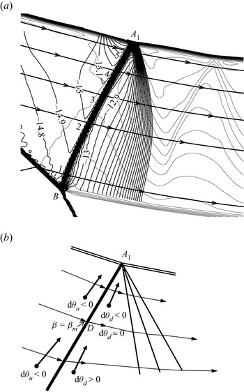
Now consider the downstream disturbance. The downstream disturbance is unknown for the present problem and we have to rely on numerical observation to have some knowledge about this downstream disturbance. The rationality of the observation will be discussed in Appendix B.5.
Figure 11(a) displays, for  $M_{0}=3$ and
 $\theta _{01}=13^{\circ }$, the numerical result of the local flow angle defined by
 $\theta _{loc}=\arctan ({v}/{u})$ (here,
 $u$ and
 $v$ are the local velocity components). We see that the contour lines of
 $\theta _{loc}$ just downstream of some segment of
 $BA_{1}$ around the point with
 ${\beta }={\beta }_{m}$ are almost parallel to the shock
 $BA_{1}$, meaning that the variation
 ${\rm d}\theta _{d}\approx 0$ so the flow streams downstream of this segment are approximately parallel. However, we have
 ${\rm d}\theta _{d}>0$ near
 $B$ and
 ${\rm d}\theta _{d}<0$ near
 $A_{1}$ if we look at figure 11(a) closely. See figure 11(b) for a schematic display of the variations of flow angles for the upper part of
 $BA_{1}$.
Local flow angle near the shock  $BA_{1}$. (a) Numerical solution of
 $\theta _{loc}$ for
 $M_{0}=3$ and
 $\theta _{01}=13^{\circ }$ (the thick lines are for
 $\theta _{loc}$ and the thin lines are for Mach number), (b) schematic display of the variations of
 $\theta _{u}$ and
 $\theta _{d}$.

Near the point with  ${\beta }={\beta }_{m}$, the sign of
 ${\rm d}\theta _{d}$ appears to be not determined but the absolute value of
 ${\rm d}\theta _{d}$ is small enough so we may assume
 ${\rm d}\theta _{d}=0$ (at the end of Appendix B.4 a possible reason is given for this assumption). Near the ends of
 $BA_{1}$ the size of
 ${\rm d}\theta _{d}$ is not negligible. The reason why we have
 ${\rm d}\theta _{d}>0$ near
 $B$ and
 ${\rm d}\theta _{d}<0$ near
 $A_{1}$ appears to be very subtle. In Appendix B.5 we will simply point out that, if we do not have
 ${\rm d}\theta _{d}<0$ near
 $A_{1}$, then the pressure continuity constraint across the slipline will be violated.
B.3. Influence factors
Now we provide, for  $BA_{1}$, expressions that relate the variation (along
 $BA_{1}$) of the local shock angle
 ${\beta }$, the downstream Mach number
 $M_{d}$ and the downstream pressure
 $p_{d}$ to the upstream and downstream disturbances
 ${\rm d}\theta _{u}=-({1}/{\varPhi _{0}})({{\rm d}p_{slip}}/{p_{slip}})$ and
 ${\rm d}\theta _{d}$. Here, variation along
 $BA_{1}$ means difference or gradient of some quantity along
 $BA_{1}$.
Let  $\theta =\theta _{d}-\theta _{u}$ be the flow deflection angle across
 $BA_{1}$. The shock angle relation for
 ${\beta }$ of
 $BA_{1}$ is given by
 \begin{equation} \theta_{d}-\theta_{u}=F(M_{u},{\beta}),\quad {}F(M,{\beta})=\arctan \frac{2\left( {M}^{2}{\sin}^{2}{\beta}-1\right) }{\left( {M}^{2}\left( \gamma+\cos{2\beta}\right) +2\right) \tan\beta} . \end{equation}
Differentiating (B4) along  $BA_{1}$ (i.e. from point
 $B$ to
 $A_{1}$), we get
 \begin{equation} {\rm d}\theta_{d}-{\rm d}\theta_{u}=G(M_{u},{\beta})\,{\rm d}{\beta}+H(M_{u},{\beta})\,{\rm d}{M}_{u}, \end{equation}
where
 \begin{equation} G(M,{\beta})=\frac{\partial F(M,{\beta})}{\partial{\beta}} ,\quad H(M,{\beta})=\frac{\partial F(M,{\beta})}{\partial{M}} . \end{equation}
Combining (B5) and (B2) to eliminate  $dM_{u}$ and using (B1) to relate
 ${\rm d}\theta _{u}$ to
 ${\rm d}p_{slip}$, we get
 \begin{equation} {\rm d}{\beta=\varOmega}_{p_{slip}}{(M}_{u}{,\beta)}\frac{{\rm d}p_{slip}}{p_{slip}}+{\varOmega }_{\theta_{d}}{(M}_{u}{,\beta)}\,{\rm d}\theta_{d},\end{equation}
where
 \begin{equation} \left
\{\begin{array}{@{}l}
{\varOmega}_{p_{slip}}{(M,\beta)}=\dfrac{1}{\varPhi_{0}(M)}\dfrac{1-H(M,{\beta})Q(M)}{G(M,{\beta})}\\
{\varOmega}_{\theta_{d}}{(M,\beta)}=\dfrac{1}{G(M,{\beta})}
\end{array}, \right.
\end{equation}
are influence factors for the shock angle due to the upstream disturbance  ${\rm d}p_{slip}$ and downstream disturbance
 ${\rm d}\theta _{d}$.
For the downstream Mach number  $M_{d}$, we differentiate
 $M_{d}=\,f_{M} (M_{u},{\beta })$ along
 $BA_{1}$ and obtain
 \begin{equation} {\rm d}M_{d}=\,F_{M}^{({\beta})}\,{\rm d}{\beta}+\,F_{M}^{({M})}\,{\rm d}{M}, \end{equation}
where
 \begin{equation} F_{M}^{({\beta})}=\frac{\partial\, f_{M}(M_{u},{\beta})}{\partial {\beta}}\quad {\rm and} \quad F_{M}^{({M})}=\frac{\partial\, f_{M}(M_{u},{\beta})} {\partial{M}}. \end{equation}
Putting (B2) and (B7) into the above relation gives
 \begin{equation} {\rm d}M_{d}=\digamma_{p_{slip}}(M_{u},\beta)\frac{{\rm d}p_{slip}}{p_{slip}} +\digamma_{\theta_{d}}(M_{u},\beta)\,{\rm d}\theta_{d},\end{equation}
where
 \begin{equation} \left
\{\begin{array}{@{}l}
\digamma{(M,\beta)=\,F_{M}^{({\beta})}\varOmega_{p_{slip}}(M,\beta)}+\dfrac
{Q(M)}{\varPhi_{0}}\,F_{M}^{({M})},\\
\digamma_{\theta_{d}}(M,\beta)=\dfrac{\,F_{M}^{({\beta})}}{G(M,{\beta})},
\end{array} \right. \end{equation}
are influence factors for Mach number.
For the downstream pressure  $p_{d}$ we differentiate
 $p_{d}=p_{u}\,f_{p} (M_{u},\beta )=p_{slip}\,f_{p}(M_{u},\beta )$ and get
 \begin{equation} {\rm d}p_{d}=\,f_{p}(M_{u},\beta)\,{\rm d}p_{slip}+p_{slip}\frac{\partial \,f_{p}(M,\beta )}{\partial M}{\rm d}M_{u}+p_{slip}\frac{\partial \,f_{p}(M,\beta)}{\partial \beta }{\rm d}\beta. \end{equation}
Using (B7) for  ${\rm d}\beta$, (B2) for
 ${\rm d}M_{u}$, we get, from the above relation,
 \begin{equation} {\rm d}\bar{p}_{d}\circeq \frac{{\rm d}p_{d}}{p_{slip}}= \varLambda_{p_{slip}}(M_{u},\beta) \frac{{\rm d}p_{slip}}{p_{slip}}+\varLambda_{\theta_{d}}(M_{u},\beta )\,{\rm d}\theta_{d},\end{equation}
where
 \begin{equation} \left \{
\begin{array}{@{}l}
\varLambda_{p_{slip}}(M,\beta)=\,f_{p}(M,\beta)+\dfrac{\partial
\,f_{p}(M,\beta )}{\partial M}
\dfrac{Q(M)}{\varPhi_{0}}+\dfrac{\partial
\,f_{p}(M,\beta)}{\partial
\beta}{\varOmega}_{p_{slip}}{(M,\beta)},\\
\varLambda_{\theta_{d}}(M,\beta)=\dfrac{\partial
\,f_{p}(M,\beta)}{\partial \beta
}\dfrac{1}{G(M,{\beta})}, \end{array} \right.
\end{equation}
are influence factors for pressure.
B.4. Role of upstream and downstream disturbances on the two segments of $BA_{1}$

The role of the preceding compression waves (i.e. the upstream disturbance) on  $BA_{1}$ can be considered by looking at the signs of the influence factors
 ${\varOmega }_{slip}$,
 $\digamma _{slip}$ and
 ${\varLambda _{slip}}$ and the role of the downstream disturbance can be considered by looking at the signs of
 ${\varOmega }_{\theta _{d}}$,
 $\digamma _{\theta _{d}}$ and
 ${\varLambda _{\theta _{d}}}$ as well as the sign of
 ${\rm d}\theta _{d}$.
The signs of  ${\varOmega _{slip}}$ and
 ${\varOmega }_{\theta _{d}}$ can be easily determined. In fact, it is easy to see that
 $H(M_{u},{\beta })={\partial F(M_{u},{\beta })}/{\partial M}>0$. Moreover,
 $Q(M_{u})<0$ according to (B3). Thus we have
 $1-H(M_{u},{\beta })Q(M_{u})>0$ and the sign of
 ${\varOmega _{slip}}$ is determined by the sign of
 $G(M_{u},{\beta })={\partial F(M_{u},{\beta })}/{\partial {\beta }}$. Using (B4), it is easily shown that for
 ${\beta >\beta }_{m}$, we have
 $G(M_{u},{\beta })<0$ and therefore
 ${\varOmega _{slip}>0}$. On the contrary, for
 ${\beta <\beta }_{m}$, we have
 $G(M_{u},{\beta })>0$ and therefore
 ${\varOmega _{slip}<0}$. The sign of
 ${\varOmega }_{\theta _{d}}$ is the sign of
 $G(M_{u},{\beta })$.
The signs for other influence factors are, however, not as evident as the signs of  ${\varOmega _{slip}}$ and
 ${\varOmega }_{\theta _{d}}$. Consider for instance
 $\digamma _{slip}$. Using the expression (2.1) for
 $f_{M}(M_{u},{\beta })$, one can show that, for the upstream Mach number
 $M_{u}$ close to
 $1$, we have
 ${F_{M}^{({M})}<0}$ and
 ${F_{M}^{({\beta })}<0}$. Since we have shown above that
 ${\varOmega _{slip}>0}$ and
 $Q(M_{u})<0$ and since
 $\varPhi _{0}>0$, we conclude that decreasing the upstream Mach number increases the downstream Mach number, decreasing the shock angle decreases the downstream Mach number and the two terms on the right-hand side of (B12) for
 $\digamma _{slip}$ have opposite signs so the sign of
 $\digamma _{slip}$ is not easily known.
We thus calculate the values of the influence factors for the specific condition  $M_{0}=3$ and
 $\theta _{01}=13^{\circ }$, using the expressions (B8), (B12) and (B15) (assuming
 $M_{u}=1.136$). The results for the points marked in figure 10(a), except for point 3 for which we take
 ${\beta =\beta }_{m}=74.4^{\circ }$, are displayed in table 2. Note that the infinite values for
 ${\varOmega }_{\theta _{d}}$,
 $\digamma _{\theta _{d}}$ and
 ${\varLambda _{\theta _{d}}}$ shown in table 2 are due to
 $G\rightarrow \pm 0$ at
 ${\beta \rightarrow \beta }_{m}$.
Influence factors at typical points along  $BA_{1}$, for
 $M_{0}=3$ and
 $\theta _{01}=13^{\circ }$.

First, consider the effect of the upstream disturbance due to the preceding compression waves with  ${\rm d}p_{slip}>0$.
According to table 2, for the strong solution part of  $BA_{1}$ (
 $\beta >\beta _{m}$), we have
 $\varOmega _{slip}<0,$
 $\digamma _{slip}>0$ and
 ${\varLambda _{slip}<0}$, which means that the upstream disturbance (preceding compression waves) can weaken this part, in the sense that it reduces
 $\beta$, increases
 $M_{d}$ and decreases
 $p_{d}$, in the direction along
 $BA_{1}$.
On the contrary, for the weak solution part of  $BA_{1}$ (
 ${\beta }_{M_{d}=1} <\beta <\beta _{m}$), the signs of the influence factors reverse, i.e.
 ${\varOmega _{slip}>0}$,
 $\digamma _{slip}<0$ and
 ${\varLambda _{slip}>0}$, meaning that the upstream disturbance (preceding compression waves) alone cannot weaken the shock further since it increases
 $\beta$, decreases
 $M_{d}$ and increases
 $p_{d}$, in the direction along
 $BA_{1}$.
Now consider the influence of the downstream disturbance.
From table 2, we have  ${\varOmega }_{\theta _{d}}<0$,
 $\digamma _{\theta _{d}}>0$ and
 ${\varLambda }_{\theta _{d}}<0$ for the strong solution part (
 ${\beta >\beta }_{m}$). Thus, the downstream disturbance also weakens the lower part of
 $BA_{1}$ if
 ${\rm d}\theta _{d}>0$. According to figure 11, we indeed have
 ${\rm d}\theta _{d}>0$ for the part of
 $BA_{1}$ well below point 3 while
 ${\rm d}\theta _{d}\approx 0$ near this point.
For the weak solution part ( ${\beta }_{M_{d}=1}<\beta <\beta _{m}$), we have
 ${\varOmega }_{\theta _{d}}>0$,
 $\digamma _{\theta _{d}}<0$ and
 ${\varLambda } _{\theta _{d}}>0$ according to table 2. Thus, if
 ${\rm d}\theta _{d}<0$, this weak solution part can be weakened by the downstream disturbance. According to figure 11, we indeed observe
 ${\rm d}\theta _{d}<0$ and the magnitude of
 ${\rm d}\theta _{d}$ becomes large when approaching
 $A_{1}$. Thus, though the upstream disturbance cannot weaken the strong solution part of
 $BA_{1}$, the downstream disturbance can, which may be the reason that the sonic condition is reached at
 $A_{1}$.
The vanishing of  ${\rm d}\theta _{d}$ at
 ${\beta \rightarrow \beta }_{m}$ may be due to the infinite values for
 ${\varOmega }_{\theta _{d}},\digamma _{\theta _{d}}$ and
 ${\varLambda _{\theta _{d}}}$ at
 ${\beta \rightarrow \beta }_{m}$, since if
 ${\rm d}\theta _{d}$ does not vanish, the products
 ${\varOmega }_{\theta _{d}}\,{\rm d}\theta _{d},\digamma _{\theta _{d}}\,{\rm d}\theta _{d}$ and
 ${\varLambda _{\theta _{d}}}\,{\rm d}\theta _{d}$ would become infinite.
B.5. Summary
The observation from numerical simulation and the simplified analysis given above appear to support the following statement for the weakening of  $BA_{1}$ and for the creation of the sonic end
 $A_{1}$.
For the strong solution part of  $BA_{1}$ (
 ${\beta >\beta }_{m}$), the upstream disturbance (due to the preceding compression waves with
 ${\rm d}p_{slip}>0$) can weaken
 $BA_{1}$ up to the point satisfying the detachment condition (
 ${\beta }={\beta }_{m}$) (say point 3 in figure 10a). While for the weak solution part (
 ${\beta }_{M_{d}=1}<\beta <\beta _{m}$), although the upstream disturbance cannot weaken the shock, the downstream disturbance can weaken it by deflecting the flow streams further toward the lower side (i.e.
 ${\rm d}\theta _{d}<0$). The combined effect of the upstream and downstream disturbances should make the flow deflection angle
 $\theta =\theta _{d} -\theta _{u}$ across
 $BA_{1}$ decrease along
 $BA_{1}$, to the extent that
 $BA_{1}$ is weakened until a sonic end is reached at
 $A_{1}$. The reason that the downstream disturbance should dominate the weakening of
 $BA_{1}$ near
 $A_{1}$ to finally create the sonic end can be associated with the pressure continuity requirement as follows.
Near  $A_{1}$ the downstream flow streams appear to update the direction until we have the required
 ${\rm d}\theta _{d}$ to create the sonic end, which then creates the sonic line emanating from
 $A_{1}$, from which, as we show in § 4.2, a subsequent expansion fan will be created to reduce the pressure downstream of the upper part of the shock to meet the pressure continuity condition across the slipline near
 $A_{1}$. Otherwise, this pressure continuity condition, as required by any two parallel flow streams separated by a slipline, will be violated.