1 Introduction
Because flying insects exhibit exceptional manoeuvrability and flight performance, the kinematic and morphological features of their wings and the physical principles of their flight capabilities have been of interest in biofluid mechanics and bio-inspired engineering. Most previous studies of insect flight have investigated continuous wings with no discontinuities due to gaps on the wing surfaces (e.g. Weis-Fogh Reference Weis-Fogh1973; Ellington et al. Reference Ellington, van den Berg, Willmott and Thomas1996; Dickinson, Lehmann & Sane Reference Dickinson, Lehmann and Sane1999). However, microscopic flying insects such as the fairyfly (Mymaridae) and thrips (Thysanoptera), which inhabit the low-Reynolds-number flow regime, have evolved bristled wings that comprise a main frame and several cylindrical bristles that extend from the main frame with gaps between them. For images of bristled wings, see George & Huber (Reference George and Huber2011), Huber & Noyes (Reference Huber and Noyes2013) and Lee, Lahooti & Kim (Reference Lee, Lahooti and Kim2018).
Microscopic hairy structures are common on the appendages of small organisms (Koehl Reference Koehl1996; Koehl et al. Reference Koehl, Koseff, Crimaldi, McCay, Cooper, Wiley and Moore2001). With decreasing Reynolds number, viscous flow around an array of hairs undergoes a notable transition so that the array changes its function from a sieve to a paddle (Umemura Reference Umemura1982; Lee & Leal Reference Lee and Leal1986; Cheer & Koehl Reference Cheer and Koehl1987). Vorticity generated on a solid surface is confined to a thin shear layer in the high-Reynolds-number flow, and the effect of viscous diffusion is not critical for aerodynamic interaction of multiple lift-generating bodies closely arranged (Kim, Lee & Kim Reference Kim, Lee and Kim2019). However, for the low-Reynolds-number flow of relatively slow surrounding fluid and narrow gaps, vorticity of the shear layers developed from the solid surface is diffused strongly away from the surface, and the diffused shear layers eventually form virtual fluid barriers in the gaps between the bodies (Nawroth et al. Reference Nawroth, Feitl, Colin, Costello and Dabiri2010). This reduces the leakage through the gaps appreciably, thereby changing how the array functions. That is, discrete solid objects of the array behave as if they were aerodynamically continuous, and mutual aerodynamic interaction by strong viscous diffusion is of great importance for the array. With this principle, micro-aerodynamic decelerators made of multiple nanofibre mats were proposed by Zussman, Yarin & Weihs (Reference Zussman, Yarin and Weihs2002) for potential applications as passive airborne platforms. In addition, it was reported recently that the porosity of the dandelion pappus tunes precisely to stabilize the vortical structure formed behind during wind dispersion, which can maximize aerodynamic loading while minimizing material requirements (Cummins et al. Reference Cummins, Seale, Macente, Certini, Mastropaolo, Viola and Nakayama2018).
The fairyfly and thrips also use virtual fluid barriers between their bristles for aerial flight. An experimental study with a scaled-up translating or rotating bristled wing reported that such a wing generated slightly lower aerodynamic force compared to that of a smooth wing with no gaps (Sunada et al. Reference Sunada, Takashima, Hattori, Yasuda and Kawachi2002). Subsequently, the aerodynamic advantages of bristled wings were studied analytically (Barta & Weihs Reference Barta and Weihs2006; Weihs & Barta Reference Weihs and Barta2008) and numerically (Davidi & Weihs Reference Davidi and Weihs2012). The virtual fluid barriers compensate for the reduced force due to the gaps and allow a bristled wing to have a higher force coefficient; here, the actual surface area is considered when defining the force coefficient. Recently, Lee & Kim (Reference Lee and Kim2017) studied the flow structure of a three-dimensional (3-D) translating bristled-wing model experimentally. They identified the Reynolds-number-dependent behaviour of the shear layers in the gaps between the bristles and how that affects the formation of leading-edge vortices and the generation of lift.
Besides simple translating motion, more complicated motion and the kinematic patterns of actual wings have been investigated. Barta (Reference Barta2011) examined theoretically a row of oscillating slender bodies in Stokes flow and presented parametric results with respect to the oscillation frequency, the number of bristles, the slenderness ratio and the space between bristles. Recently, Lee et al. (Reference Lee, Lahooti and Kim2018) investigated the vortices generated within the gaps of a flapping bristled wing, with particular emphasis on the phase of stroke reversal; they showed that the flow in the gaps responds faster to wing motion as the Reynolds number decreases. Santhanakrishnan et al. (Reference Santhanakrishnan, Robinson, Jones, Lowe, Gadi, Hedrick and Miller2014) modelled a bristled wing as a porous membrane wing and showed that in wing–wing interaction through the clap-and-fling mechanism, flow leakage through the wing surfaces reduces the drag required to fling the wings apart; a pair of porous wings can therefore achieve a large lift-to-drag ratio over a flapping cycle. This study was extended to a numerical simulation of a two-dimensional (2-D) bristled wing (Jones et al. Reference Jones, Yun, Hedrick, Griffith and Miller2016) and an experimental study of a 3-D bristled wing (Kasoju et al. Reference Kasoju, Terrill, Ford and Santhanakrishnan2018).
While previous studies have considered the Reynolds number and the gap width as the main independent parameters regarding the aerodynamic effects of gaps, the underlying principles of optimizing the configuration of a bristled wing to enhance its aerodynamic force remain unclear despite their importance in bio-inspired applications. In the present study, as the first step in a new approach to analysing aerodynamic force generation and revealing the combined effects of the dynamic and kinematic parameters (i.e. Reynolds number and gap width), we investigate numerically how the aerodynamic force and flow structure of a 2-D bristled wing fixed in space vary over wide ranges of the Reynolds number and gap width. Unlike an infinite-Reynolds-number solution, where the aerodynamics are characterized by the diameter of each bristle, the aerodynamics in the low-Reynolds-number regime depend on the gap width because the viscous diffusion across the gap between the bristles is of great importance. That is, the Reynolds number based on the gap width is a governing parameter in the low-Reynolds-number regime. With this in mind, we propose new insights into the characteristics of the drag and lift acting on each bristle and the entire wing. We then compare the aerodynamic forces predicted by a simple but reliable theoretical model with those obtained by numerical simulations to assess whether our approach is effective for finding the optimal configuration.
2 Problem description
2.1 Bristled-wing model
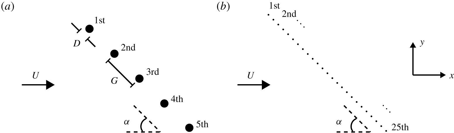
Schematic diagrams of (a) five-bristle model and (b) 25-bristle model.

We introduce simplified 2-D bristled-wing models that capture the features of a biological bristled wing as used by Jones et al. (Reference Jones, Yun, Hedrick, Griffith and Miller2016) and Lee et al. (Reference Lee, Lahooti and Kim2018). As a preliminary exploration of the effects of the Reynolds number and the gap size, we begin by considering a simple five-bristle model, which consists of five equally spaced cylinders (bristles) of identical diameter  $D$, aligned in a straight line (figure 1a). Admittedly, the number of bristles is smaller than that of the actual bristled wing found in nature. To confirm whether the main findings from the five-bristle model can be generalized, we also examine a 25-bristle model with 25 equally spaced bristles of equal diameter
 $D$ in a straight line (figure 1b).
We define the gap width  $G$ as the distance between the centres of two adjacent bristles. The Reynolds number
 $Re_{D}~(=\unicode[STIX]{x1D70C}UD/\unicode[STIX]{x1D707})$ based on the bristle diameter ranges between 0.01 and 1.0, i.e.
 $Re_{D}=[0.01,0.02,0.05,0.1,0.2,0.5,1.0]$; here,
 $U$ is the free-stream velocity,
 $\unicode[STIX]{x1D70C}$ is the fluid density and
 $\unicode[STIX]{x1D708}~(=\unicode[STIX]{x1D707}/\unicode[STIX]{x1D70C})$ is the fluid kinematic viscosity. For both five-bristle and 25-bristle models, the normalized gap width between two adjacent bristles is
 $G/D=3$–2000. By the definitions of
 $G$ and
 $D$ (figure 1a),
 $G/D=1$ means the bristles are in contact. The large variations in the orders of
 $Re_{D}$ and
 $G/D$ are intended to find the optimal configuration of the model regarding lift generation.
For both models, we define an angle of attack  $\unicode[STIX]{x1D6FC}$ as the angle between the straight line connecting the bristles and the
 $x$ axis parallel to the direction of the free stream (figure 1). For the five-bristle model,
 $\unicode[STIX]{x1D6FC}$ varies from
 $15^{\circ }$ to
 $90^{\circ }$, i.e.
 $\unicode[STIX]{x1D6FC}=[15^{\circ },30^{\circ },45^{\circ },60^{\circ },70^{\circ },90^{\circ }]$ (figure 1a). For the 25-bristle model,
 $\unicode[STIX]{x1D6FC}$ is fixed to be
 $45^{\circ }$ (figure 1b).
2.2 Numerical method
Comparison of drag coefficients ( $C_{d}=2F/\unicode[STIX]{x1D70C}U^{2}D$) for a circular cylinder in a uniform free stream.

The 2-D incompressible laminar flow around a bristle model is solved numerically using OpenFOAM. We use the simpleFoam solver for steady-state solutions and the second-order Gauss-linear scheme for spatial discretizations, and we set the time derivative as zero for steady-state solutions in low-Reynolds-number flow. Although the kinematics of an actual wing are unsteady, in this study, we focus on revealing the steady aerodynamic performance of the model and thus consider steady-state solutions.
For our numerical simulations, we construct the rectangular fluid domain  $[-2.5\times 10^{5}D,2.5\times 10^{5}D]\times [-2.5\times 10^{5}D,2.5\times 10^{5}D]$ and 10 layers of structured grids near each bristle. The grid size next to a bristle is fixed as
 $0.01D$. Outside the structured layers, we construct triangular grids of exponentially increasing size with the growth ratio of 1.05 for the rectangular region that encompasses all the bristles; the size of this region depends on the gap size or the number of bristles. Finally, we construct structured grids of exponentially increasing size with the growth ratio of 1.05 for the rest of the fluid domain. The total number of cells is less than
 $1.0\times 10^{6}$ for the 25-bristle model and varies slightly depending on the gap size and the number of bristles. To check grid convergence, we change the minimum size of the grid from
 $0.01D$ to
 $0.02D$ while keeping all other conditions the same. At
 $Re_{D}=0.1$, the values of the drag coefficient
 $C_{d}=2F/\unicode[STIX]{x1D70C}U^{2}D$ for a circular cylinder in a uniform free stream derived from the fine-grid and coarse-grid cases differ little, being
 $C_{d}=56.1$ and 56.0, respectively. This result justifies our decision to use
 $0.01D$ as the minimum grid size.
For validation of our numerical method, we conduct numerical simulations to obtain the values of the drag coefficient  $C_{d}$ for a circular cylinder in a uniform free stream for
 $Re_{D}$ ranging between 0.01 and 1.0. Table 1 compares our results with numerical results by Khalili & Liu (Reference Khalili and Liu2017) and shows that our results are consistent with their results for
 $Re_{D}\leqq 1$.
3 Results and discussion
3.1 Aerodynamic characteristics of five-bristle model
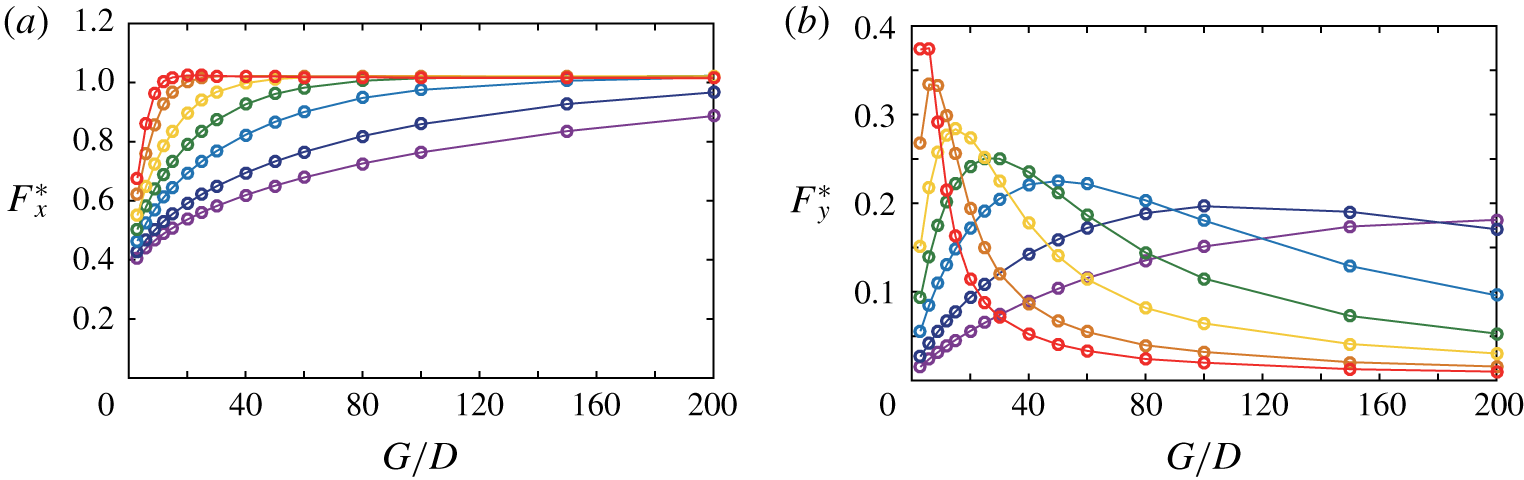
(a) Drag force and (b) lift force of the uppermost (first) bristle in the five-bristle model at  $\unicode[STIX]{x1D6FC}=90^{\circ }$ for
 $Re_{D}=1$ (red), 0.2 (orange), 0.5 (yellow), 0.1 (green), 0.05 (blue), 0.02 (navy) and 0.01 (purple). Note that the vertical range differs between panels (a) and (b).

We first begin by considering the five-bristle model at  $\unicode[STIX]{x1D6FC}=90^{\circ }$ (figure 1a) to determine how the gap size
 $G/D$ and the Reynolds number
 $Re_{D}$ affect the aerodynamic forces and corresponding flow structures. We then extend the main findings for the five-bristle model at
 $\unicode[STIX]{x1D6FC}=90^{\circ }$ to the five-bristle model with other angles of attack, and furthermore to the 25-bristle model. The
 $x$-directional force
 $F_{x}$ (drag) and the
 $y$-directional force
 $F_{y}$ (lift) acting on the first uppermost bristle are normalized by the drag force
 $F_{x,s}$ of a single isolated bristle obtained at the same
 $Re_{D}$:
 $$\begin{eqnarray}F_{x}^{\ast }=F_{x}/F_{x,s}\quad \text{and}\quad F_{y}^{\ast }=F_{y}/F_{x,s}.\end{eqnarray}$$
Note that  $F_{y}$ is normalized by
 $F_{x,s}$ because the lift
 $F_{y,s}$ of the single isolated bristle is zero. The normalized drag
 $F_{x}^{\ast }$ and lift
 $F_{y}^{\ast }$ of the first bristle in the five-bristle model at
 $\unicode[STIX]{x1D6FC}=90^{\circ }$ are provided for
 $Re_{D}=0.01$–1 in figure 2. Because the flow is symmetric with respect to the third bristle for low-Reynolds-number flow, we show the forces for the first bristle only. Although the forces on the second bristle are not presented, they follow similar trends to the first bristle, with minor differences in their magnitudes (see figure 7a,b later). For the first bristle
 $F_{x}^{\ast }$ approaches that of the single bristle asymptotically as either
 $Re_{D}$ or
 $G/D$ increases (figure 2a). The
 $F_{x}^{\ast }$ value converges to unity at smaller
 $G/D$ for higher
 $Re_{D}$. For instance, for
 $Re_{D}=1$,
 $F_{x}^{\ast }$ reaches unity at
 $G/D<20$, whereas for
 $Re_{D}=0.01$, it remains below 0.9 even at
 $G/D>200$.
At  $\unicode[STIX]{x1D6FC}=90^{\circ }$, the first and second bristles experience lifts that are equal in magnitude and opposite in sign to the fifth and fourth bristles, respectively: positive lifts for the first and second bristles, and negative lifts for the fourth and fifth bristles. Note that no lift is found for the third bristle because of the symmetry of flow. For given
 $Re_{D}$,
 $F_{y}^{\ast }$ of the first bristle tends to increase and then decrease with
 $G/D$, thereby having a peak (figure 2b). After the peak,
 $F_{y}^{\ast }$ asymptotes to zero as
 $G/D$ goes to infinity. The maximum
 $F_{y}^{\ast }$ occurs at smaller
 $G/D$ for higher
 $Re_{D}$. Compare
 $Re_{D}=0.2$ and
 $Re_{D}=0.02$ in figure 2(b), for which the values of
 $G/D$ corresponding to maximum lift are approximately 15 and 100, respectively.
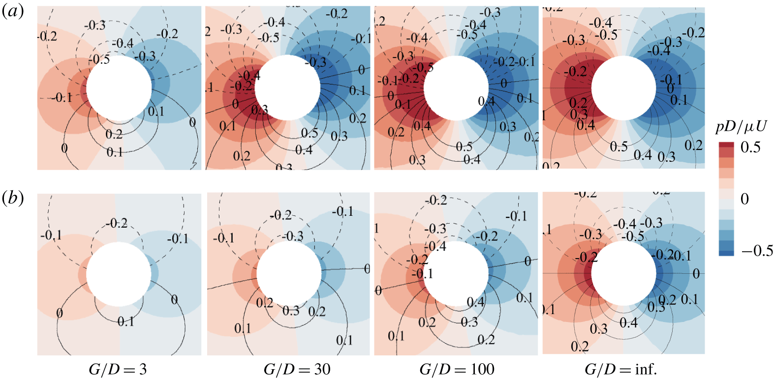
Pressure and vorticity contours around the first bristle of the five-bristle model at  $\unicode[STIX]{x1D6FC}=90^{\circ }$ for
 $Re_{D}=0.1$ (a) and 0.01 (b). The dashed and solid contour lines denote negative and positive vorticities (
 $\unicode[STIX]{x1D714}D/U$), respectively, and
 $G/D=\text{inf.}$ indicates the case of a single isolated cylinder.

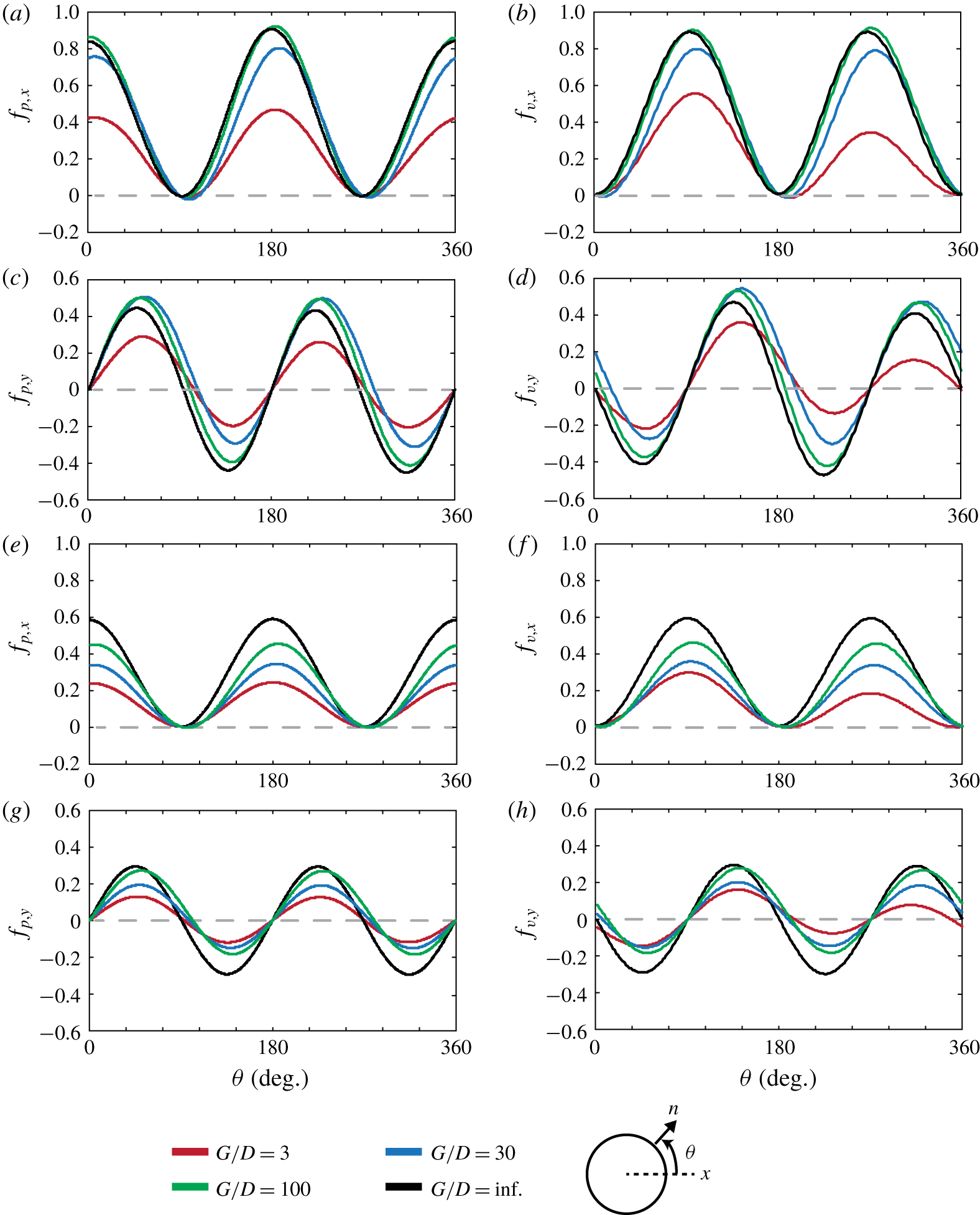
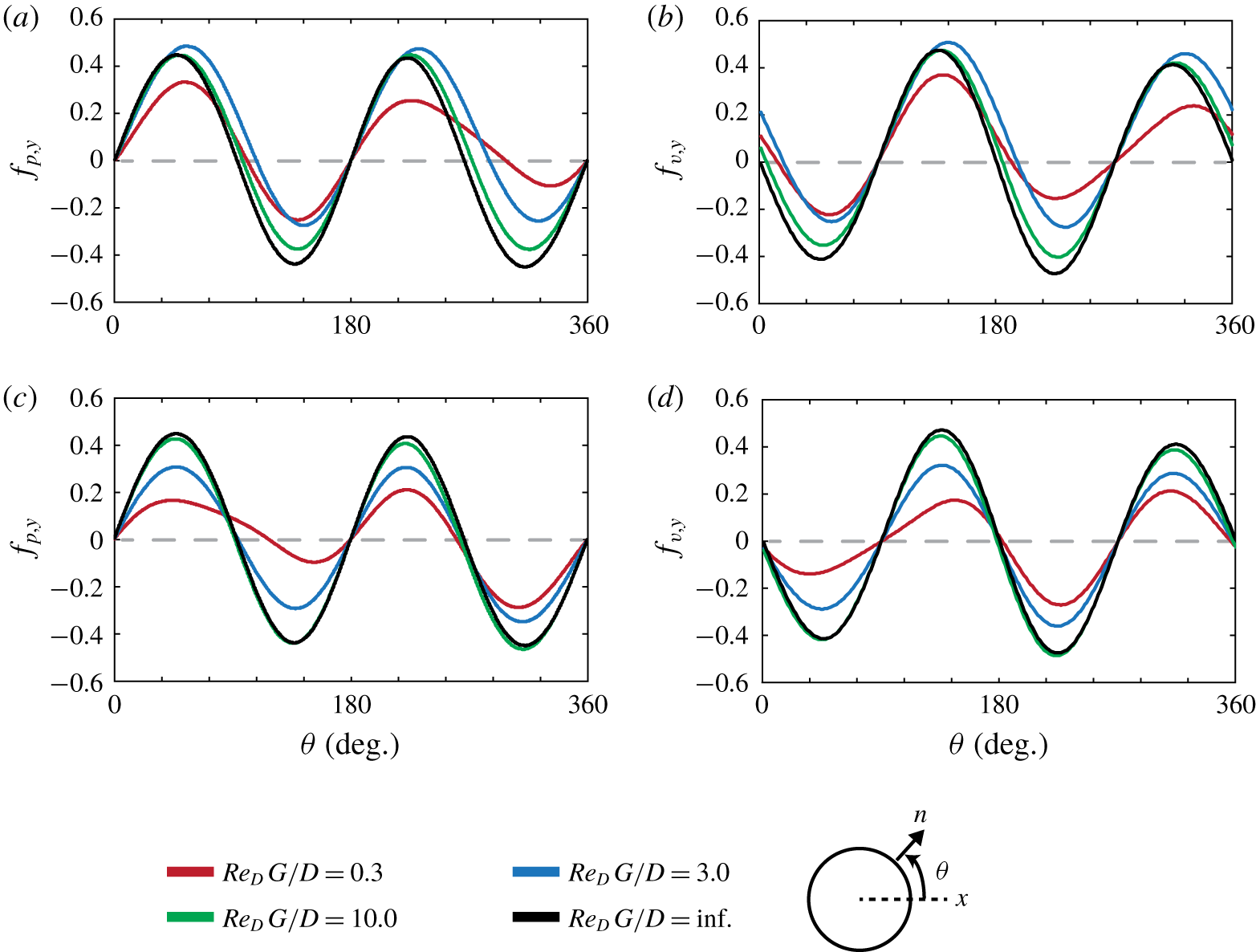
Spatial distributions of forces due to pressure and viscous stress per unit surface area acting on the surface of the first bristle in the five-bristle model at  $\unicode[STIX]{x1D6FC}=90^{\circ }$ for (a–d)
 $Re_{D}=0.1$ and (e–h)
 $Re_{D}=0.01$.

To correlate the aforementioned force variation with the flow structure, we examine the force distributions on the surface of the first bristle as well as the pressure and vorticity fields around it (figures 3 and 4). We decompose the force  $\boldsymbol{F}$ exerted on a bristle into two components, force due to pressure and force due to viscous stress, i.e.
 $$\begin{eqnarray}\boldsymbol{F}=\int _{S}-p\boldsymbol{n}\,\text{d}S+\int _{S}\boldsymbol{n}\boldsymbol{\cdot }\unicode[STIX]{x1D749}\,\text{d}S,\end{eqnarray}$$
where  $\boldsymbol{n}$ is the unit normal vector into the fluid domain,
 $p$ is the pressure,
 $\unicode[STIX]{x1D749}$ is the viscous stress tensor and
 $S$ is the surface of the bristle. Note that the viscous stress tensor on the surface is related to the vorticity thereon as
 $\boldsymbol{n}\boldsymbol{\cdot }\unicode[STIX]{x1D749}=-\unicode[STIX]{x1D707}\boldsymbol{n}\times \unicode[STIX]{x1D74E}$, which is why we examine the vorticity field in figure 3. Both the pressure force
 $-p\boldsymbol{n}$ per unit surface area and the viscous force
 $\boldsymbol{n}\boldsymbol{\cdot }\unicode[STIX]{x1D749}$ per unit surface area are non-dimensionalized by
 $D$,
 $\unicode[STIX]{x1D707}$ and
 $U$, respectively:
 $-p\boldsymbol{n}D/\unicode[STIX]{x1D707}U$ and
 $\boldsymbol{n}\boldsymbol{\cdot }\unicode[STIX]{x1D749}D/\unicode[STIX]{x1D707}U$. To examine how they contribute to the
 $x$- and
 $y$-directional forces, we denote
 $f_{p,x}$ and
 $f_{p,y}$ as the
 $x$- and
 $y$-directional components of
 $-p\boldsymbol{n}D/\unicode[STIX]{x1D707}U$, respectively. Likewise, we denote
 $f_{v,x}$ and
 $f_{v,y}$ as the
 $x$- and
 $y$-directional components of
 $\boldsymbol{n}\boldsymbol{\cdot }\unicode[STIX]{x1D749}D/\unicode[STIX]{x1D707}U$, respectively. Because in creeping flow the viscous and pressure forces are comparable, these two force components should be considered together.
We begin with the smallest gap  $G/D=3$, for which
 $F_{x}^{\ast }$ is reduced significantly; e.g.
 $F_{x}^{\ast }=0.50$ at
 $Re_{D}=0.1$ and
 $F_{x}^{\ast }=0.41$ at
 $Re_{D}=0.01$ (figure 2). For
 $Re_{D}=0.1$ and 0.01, both the pressure and the vorticity around the bristles become considerably weaker than those of a single isolated bristle (
 $G/D=\text{inf.}$), thereby reducing the magnitudes of the drag components
 $f_{p,x}$ and
 $f_{v,x}$ (figures 3 and 4). Interestingly, the
 $x$ component
 $f_{v,x}$ of the viscous force is reduced more notably on the lower surface of the bristle (
 $\unicode[STIX]{x1D703}=180^{\circ }$–
 $360^{\circ }$). For
 $G/D=3$ and
 $Re_{D}=0.1$, the maximum values of
 $f_{v,x}$ on the upper and lower surfaces are 0.56 and 0.35, respectively. Meanwhile, the
 $x$ component
 $f_{p,x}$ of the pressure force is reduced almost equally on the windward and leeward surfaces (figure 4a,b). An asymmetrically distributed viscous force and a symmetrically distributed pressure force are also found for the
 $y$ components
 $f_{p,y}$ and
 $f_{v,y}$ (figure 4c,d). Similar trends at
 $G/D=3$ and
 $Re_{D}=0.01$ are found for all of the force components (figure 4e–h).
As the gap increases beyond  $G/D=3$, the pressure gradient and vorticity around the bristle become stronger (figure 3), and correspondingly the magnitudes of the surface forces grow gradually and approach those of the single isolated bristle (figure 4). The difference in
 $f_{v,x}$ between the upper and lower surfaces of the bristle diminishes with
 $G/D$ (figure 4b,f). Similarly, the difference in
 $f_{v,y}$ between the windward and leeward surfaces reduces with
 $G/D$ (figure 4d,h). Even for the large gap width of
 $G/D=100$, however, significant deviations between the curves for
 $G/D=100$ and
 $G/D=\text{inf.}$ are still noted at
 $Re_{D}=0.01$ (figure 4e–h). This implies that, even if the bristles are separated by the same distance, they are more aerodynamically coupled when the Reynolds number is smaller; e.g., for
 $G/D=100$,
 $F_{x}^{\ast }=1.0$ at
 $Re_{D}=0.1$ and
 $F_{x}^{\ast }=0.76$ at
 $Re_{D}=0.01$ (figure 2).
Another notable feature of the flow structure is that the incident flow is deflected in such a way that the bristles repel each other. The incoming flow is deflected upwards for the upper (first and second) bristles and downwards for the lower (fourth and fifth) bristles. Accordingly, the pressure and vorticity fields around the upper bristles are tilted slightly in the anticlockwise direction, thereby generating lift (figure 3). To quantify how much the flow field is tilted compared to that of the single isolated cylinder, we draw a line connecting the two points on the bristle surface where the vorticity is zero and define the tilting angle  $\unicode[STIX]{x1D703}_{t}$ as the angle between this line and the
 $x$ axis. For
 $\unicode[STIX]{x1D703}_{t}$, we could alternatively take the angle between the
 $x$ axis and the line connecting the two points on the bristle surface at which the pressure is maximum or minimum. The tilting angles computed by these two definitions differ slightly, and hereinafter we use the former definition involving the line connecting the points of zero vorticity.
The tilting angle  $\unicode[STIX]{x1D703}_{t}$ is closely related with the lift force; this correlation is observed no matter which definition of
 $\unicode[STIX]{x1D703}_{t}$ is used. For
 $Re_{D}=0.1$, the tilting angle is greatest at
 $G/D=30$, at which value the lift is greatest (figure 2b): we have
 $\unicode[STIX]{x1D703}_{t}=10^{\circ }$ at
 $G/D=3$,
 $\unicode[STIX]{x1D703}_{t}=16^{\circ }$ at
 $G/D=30$ and
 $\unicode[STIX]{x1D703}_{t}=6^{\circ }$ at
 $G/D=100$. Because of the tilting, the negative peaks of
 $f_{p,y}$ and
 $f_{v,y}$ are roughly
 $65\,\%{-}70\,\%$ of those of the single isolated bristle at
 $G/D=30$, while the corresponding positive peaks are similar to those of the single isolated bristle (figure 4c,d). For much larger gap size, namely
 $G/D=100$, which exhibits less tilting, the positive peaks of
 $f_{p,y}$ and
 $f_{v,y}$ do not change from those of
 $G/D=30$. Meanwhile, the negative peaks approach those of the single bristle, thereby reducing the lift.
3.2 Effective gap width of five-bristle model
3.2.1 Five-bristle model at  $\unicode[STIX]{x1D6FC}=90^{\circ }$

In § 3.1, we showed that the forces exerted on a bristle depend strongly on both  $G/D$ and
 $Re_{D}$. In fact, there have been previous studies of the aerodynamic interaction of multiple bodies caused by strong viscous effects, although they did not discuss in detail how the pressure and viscous surface forces vary with gap width and Reynolds number (Barta & Weihs Reference Barta and Weihs2006; Lee et al. Reference Lee, Lahooti and Kim2018). In those previous studies,
 $Re_{D}$ and
 $G/D$ were treated independently. However, based on our results in § 3.1, we conjecture that the two parameters are coupled aerodynamically in that increasing
 $G/D$ has the same effect as increasing
 $Re_{D}$ in terms of force generation (figure 2).
To evaluate the combined effects of  $G/D$ and
 $Re_{D}$, we begin by examining the Reynolds-number-dependent spatial scale of 2-D creeping flow around a single isolated bristle (cylinder). Analytical approximations exist for flow around a cylinder at Reynolds numbers less than unity. For example, Proudman & Pearson (Reference Proudman and Pearson1957) used the method of matched asymptotic expansions to match the inner Stokes solution to the outer Oseen solution, and vice versa. In the Stokes solution, a convective term in the governing equation is neglected, while the Oseen solution considers a linearized convective term in the governing equation. According to Proudman & Pearson (Reference Proudman and Pearson1957), the Oseen solution for the streamfunction
 $\unicode[STIX]{x1D713}$ over a cylinder in polar coordinates is the expansion
 $$\begin{eqnarray}\unicode[STIX]{x1D713}=\unicode[STIX]{x1D713}_{0}(r^{\ast }Re_{D},\unicode[STIX]{x1D703})+F_{1}(Re_{D})\unicode[STIX]{x1D713}_{1}(r^{\ast }Re_{D},\unicode[STIX]{x1D703})+F_{2}(Re_{D})\unicode[STIX]{x1D713}_{2}(r^{\ast }Re_{D},\unicode[STIX]{x1D703})+\cdots \,,\end{eqnarray}$$
where  $Re_{D}=UD/\unicode[STIX]{x1D708}$ and
 $r^{\ast }$ is the dimensionless radial coordinate normalized by the cylinder radius:
 $r^{\ast }=r/R=2r/D$. The term
 $F_{n+1}(Re_{D})/F_{n}(Re_{D})$ vanishes as
 $Re_{D}$ approaches zero, making the higher-order terms negligible. For the Oseen expansion in (3.3), we use the Oseen variable
 $\hat{r}=r^{\ast }Re_{D}$ so that the radial coordinate
 $r$ is scaled by the viscous dimension
 $\unicode[STIX]{x1D708}/U$, i.e.
 $\hat{r}=2rU/\unicode[STIX]{x1D708}$. This expansion matches the Stokes region of the flow asymptotically at
 $r^{\ast }=O(1)$. Van Dyke (Reference Van Dyke1975) showed that, for small
 $\hat{r}$, the Oseen expansion can be approximated as
 $$\begin{eqnarray}\unicode[STIX]{x1D713}\approx \frac{UR}{Re_{D}}\left[\hat{r}\sin \unicode[STIX]{x1D703}+\unicode[STIX]{x1D6E5}(Re_{D})\left\{\left(\ln \frac{\hat{r}}{8}+\unicode[STIX]{x1D6FE}-1\right)\hat{r}\sin \unicode[STIX]{x1D703}+O(\hat{r}^{2}\ln \hat{r})+\cdots \,\right\}+\cdots \,\right],\quad\end{eqnarray}$$
where  $\unicode[STIX]{x1D6FE}=0.5772$ is Euler’s constant and
 $\unicode[STIX]{x1D6E5}(Re_{D})=(\text{ln}(8/Re_{D})-\unicode[STIX]{x1D6FE}+0.5)^{-1}$. See also Proudman & Pearson (Reference Proudman and Pearson1957) and Van Dyke (Reference Van Dyke1975) for detailed procedures for the solution of the creeping flow around a cylinder. The first term on the right-hand side of (3.4) represents the uniform free stream, and the second term describes the disturbance fields produced by the cylinder when the higher-order terms are neglected. Its Reynolds-number-dependent constant
 $\unicode[STIX]{x1D6E5}(Re_{D})$ decreases with
 $Re_{D}$, thereby reducing the magnitude of disturbances. As well as the streamfunction disturbance, the velocity disturbance should depend on
 $\hat{r}~(=r^{\ast }Re_{D})$, i.e.
 $u_{r}=\unicode[STIX]{x2202}\unicode[STIX]{x1D713}/r\unicode[STIX]{x2202}\unicode[STIX]{x1D703}$ and
 $u_{\unicode[STIX]{x1D703}}=-\unicode[STIX]{x2202}\unicode[STIX]{x1D713}/\unicode[STIX]{x2202}r$. That is, regarding the velocity disturbance,
 $Re_{D}^{-1}$ is an appropriate characteristic scale for the dimensionless length
 $r^{\ast }$ of the creeping flow around the bristle (Van Dyke Reference Van Dyke1975).
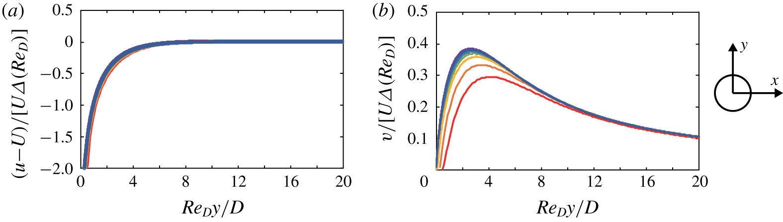
Profiles of (a)  $x$-directional and (b)
 $y$-directional velocity disturbances around a single isolated bristle on positive
 $y$ axis, which are normalized by the free-stream velocity
 $U$ and
 $\unicode[STIX]{x1D6E5}(Re_{D})=(\text{ln}(8/Re_{D})-\unicode[STIX]{x1D6FE}+0.5)^{-1}$. The scaled distance
 $Re_{D}\,y/D$ is used instead of
 $y/D$. The plots are for
 $Re_{D}=1$ (red), 0.2 (orange), 0.5 (yellow), 0.1 (green), 0.05 (blue), 0.02 (navy) and 0.01 (purple).

As given by our numerical simulation, the profiles of the velocity disturbance caused by a single isolated bristle on the positive  $y$ axis are depicted in figure 5. Because we have the Reynolds-number-dependent constant
 $\unicode[STIX]{x1D6E5}(Re_{D})$ in the second term of (3.4), the velocity disturbances
 $u-U$ and
 $v$ are normalized by
 $\unicode[STIX]{x1D6E5}(Re_{D})$ as well as the free-steam velocity
 $U$ in figure 5:
 $(u-U)/[U\unicode[STIX]{x1D6E5}(Re_{D})]$ and
 $v/[U\unicode[STIX]{x1D6E5}(Re_{D})]$. Also,
 $y/D$ is divided by
 $Re_{D}^{-1}$ to introduce a new scaled
 $y$ coordinate
 $Re_{D}\,y/D$ in figure 5.
The velocity profiles in figure 5 are determined by the scaled distance  $Re_{D}\,y/D$ regardless of the Reynolds number. Although the Reynolds numbers considered in figure 5 differ by two orders of magnitude, i.e.
 $Re_{D}=0.01$–1, the curves of the normalized
 $x$-velocity disturbance
 $(u-U)/[U\unicode[STIX]{x1D6E5}(Re_{D})]$ collapse onto a single curve: thus
 $(u-U)/[U\unicode[STIX]{x1D6E5}(Re_{D})]$ converges to zero near
 $Re_{D}\,y/D\approx 6$; and
 $u$ becomes similar to
 $U$. The curves of the normalized
 $y$-velocity disturbance
 $v/[U\unicode[STIX]{x1D6E5}(Re_{D})]$ have similar shapes but show notable deviation at low
 $Re_{D}\,y/D$, in particular for the curves of relatively large
 $Re_{D}$. Despite such deviation, the peaks of the
 $v/[U\unicode[STIX]{x1D6E5}(Re_{D})]$ curves appear in a very narrow range of
 $Re_{D}\,y/D$, between 2.6 for
 $Re_{D}=0.01$ and 4.3 for
 $Re_{D}=1.0$.


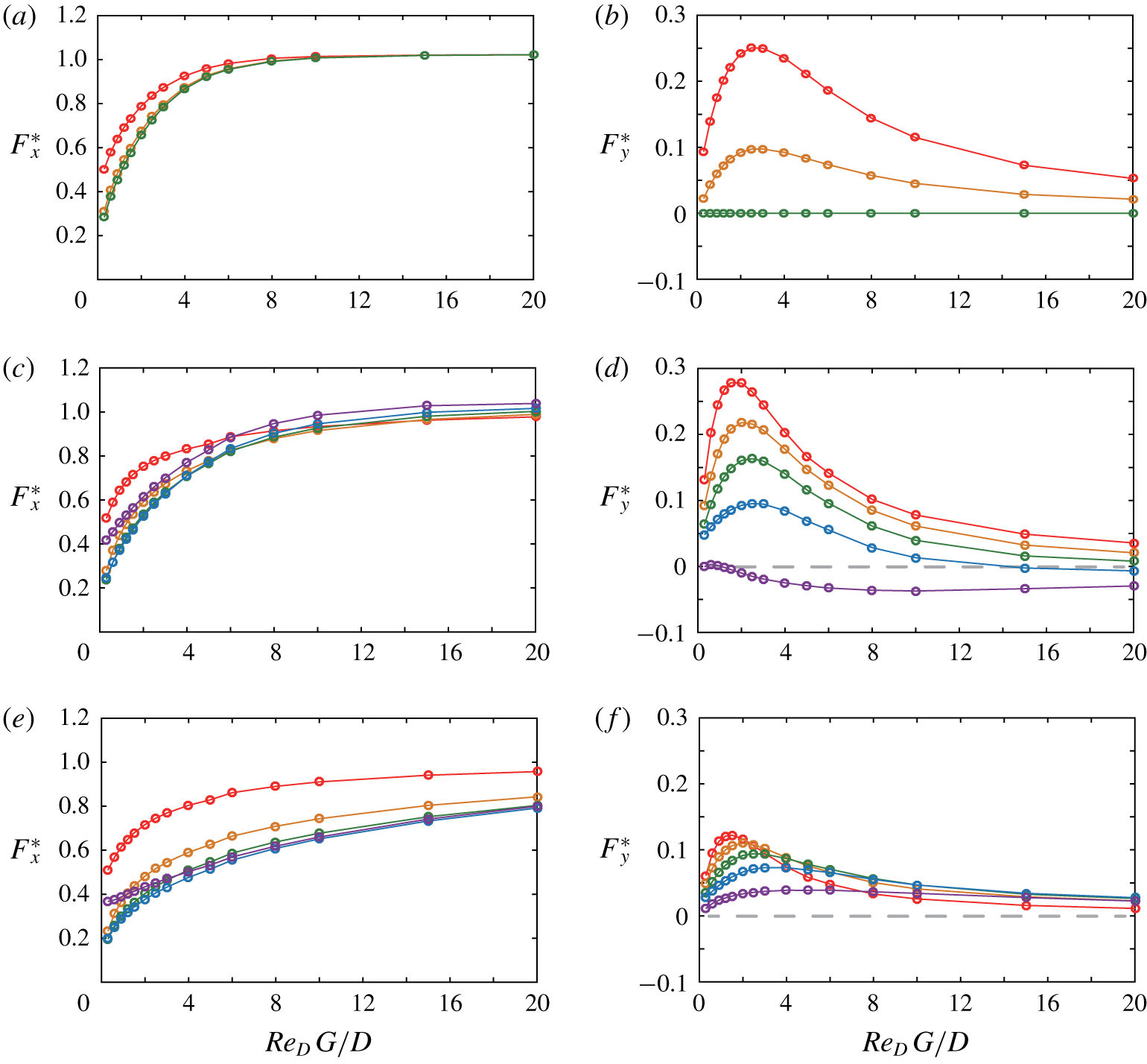
Drag and lift forces for individual bristles in the five-bristle model for $Re_{D}=0.1$: (a,b)
 $\unicode[STIX]{x1D6FC}=90^{\circ }$; (c,d)
 $\unicode[STIX]{x1D6FC}=45^{\circ }$; and (e,f)
 $\unicode[STIX]{x1D6FC}=15^{\circ }$. First bristle (red), second bristle (orange), third bristle (green), fourth bristle (blue) and fifth bristle (purple).

Given the linearity of creeping flow, the spatial scale of the flow around each bristle in the five-bristle model may be the same as that for the single isolated bristle. Furthermore, given that the velocity profile is characterized by  $Re_{D}\,y/D$, the lift and drag forces
 $F_{x}^{\ast }$ and
 $F_{y}^{\ast }$ acting on each bristle may be predicted similarly by the scaled gap width
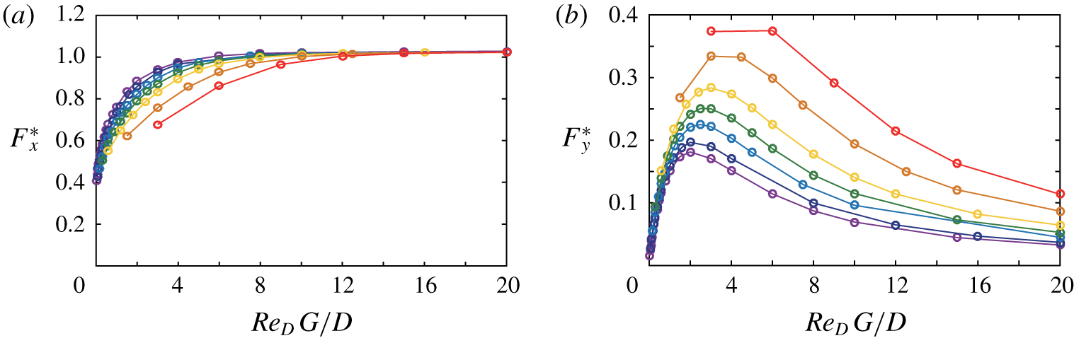
 $Re_{D}\,G/D$. Figure 2 is replotted as figure 6 with the scaled gap width
 $Re_{D}\,G/D$ instead of
 $G/D$. For different values of
 $Re_{D}$ between 0.01 and 1, the curves of
 $F_{x}^{\ast }$ show a consistent pattern and reside in the narrow range of 0.85–1.0 for
 $Re_{D}\,G/D\geqslant 6$. More interestingly, all the curves of
 $F_{y}^{\ast }$ exhibit a peak at
 $Re_{D}\,G/D\approx 3$. Figure 6 shows that how the forces vary is determined by a single parameter
 $Re_{D}\,G/D$ that combines the effects of the Reynolds number and the gap size for low-Reynolds-number flow. In fact,
 $Re_{D}\,G/D$ is equal to the Reynolds number
 $Re_{G}~(=UG/\unicode[STIX]{x1D708})$ based on the gap width
 $G$ as the characteristic length. However, to emphasize the combined effect of the two representative variables
 $Re_{D}$ and
 $G/D$, we use
 $Re_{D}\,G/D$ rather than
 $Re_{G}$ in this study and name it ‘effective gap width’.
The aforementioned results offer insight into elucidating a clear difference between two asymptotic solutions: the very-low-Reynolds-number solution in which the array of bristles is impervious, and the infinite-Reynolds-number solution in which the bristles are aerodynamically independent of each other unless they are very close to each other. Aerodynamic performance is characterized by the diameter  $D$ of each bristle, i.e.
 $Re_{D}$, at the high Reynolds number of
 $Re_{D}\gg 1$. However, at the low Reynolds number of
 $Re_{D}\leqslant 1$, viscous diffusion across the gap between the bristles is of great importance, and thus aerodynamic performance is determined by the gap width
 $G$ between the bristles, i.e.
 $Re_{G}~(=Re_{D}\,G/D)$ rather than the bristle diameter
 $D$. As the Reynolds number decreases below
 $Re_{D}=1$, the flow field converges asymptotically, and aerodynamic characterization by the effective gap width
 $Re_{D}\,G/D$ should be better suited. Indeed, in figures 5 and 6, with decreasing
 $Re_{D}$, the curves tend to collapse towards the asymptotic solution of very low Reynolds number. The streamwise velocity component converges to the asymptotic solution faster than the cross-flow velocity component (figure 5). Similarly, the drag strongly affected by the streamwise velocity component converges faster than the lift relevant to the cross-flow velocity component (figure 6).
3.2.2 Five-bristle model at $\unicode[STIX]{x1D6FC}<90^{\circ }$

Based on our analysis of the five-bristle model at  $\unicode[STIX]{x1D6FC}=90^{\circ }$, here we further consider the five-bristle model with various angles of attack (figure 1a), to confirm whether the performance of the five-bristle model can be characterized by the effective gap width
 $Re_{D}\,G/D$ for a wide range of the angle of attack. First, the lift and drag trends of each bristle are examined for three angles of attack,
 $\unicode[STIX]{x1D6FC}=90^{\circ },45^{\circ }$ and
 $15^{\circ }$, and the Reynolds number
 $Re_{D}=0.1$ as representative cases (figure 7). Note that data for
 $\unicode[STIX]{x1D6FC}=90^{\circ }$ examined in § 3.2.1 are included in figure 7 for comparison. Although not presented here, we found that the overall trends were not altered notably by the change in the Reynolds number for the entire range of
 $\unicode[STIX]{x1D6FC}$ and accordingly chose a single Reynolds number
 $Re_{D}=0.1$ for figure 7. For
 $\unicode[STIX]{x1D6FC}=90^{\circ }$, the forces exerted on each bristle depend on its relative position within the wing. As we mentioned in § 3.1, a bristle near the outer edge of the wing experiences greater drag and lift than do the inner bristles near the centre of the wing because the incoming flow decelerates in front of the inner bristles due to the formation of a virtual fluid barrier with the gaps (Lee et al. Reference Lee, Lahooti and Kim2018). In our simulations for
 $Re_{D}=0.1$, the values of
 $F_{x}^{\ast }$ for the first and second bristles are 0.87 and 0.80, respectively, at
 $Re_{D}\,G/D=3.0$. For the same
 $Re_{D}$ and
 $Re_{D}\,G/D$, the values of
 $F_{y}^{\ast }$ for the first and second bristles are 0.25 and 0.097, respectively (figure 7a,b). Because of the symmetric flow, the curves for the fourth and fifth bristles are not included in figure 7(a,b).
For  $\unicode[STIX]{x1D6FC}=45^{\circ }$, in contrast to
 $\unicode[STIX]{x1D6FC}=90^{\circ }$, the drag of the first bristle that faces the free stream head-on is larger than that of the fifth bristle at the trailing edge up to
 $Re_{D}\,G/D\approx 6$ (figure 7c). In the range of
 $Re_{D}\,G/D$, the drag force of the first bristle is greatest among the five. For example, for
 $Re_{D}\,G/D=0.3$, the values of
 $F_{x}^{\ast }$ for the first and fifth bristles are 0.52 and 0.42, respectively. The values of
 $F_{x}^{\ast }$ for the remaining bristles lie in the range 0.24–0.28, much smaller than for the outermost bristles. As
 $Re_{D}\,G/D$ increases, the difference in
 $F_{x}^{\ast }$ among all bristles decreases, and
 $F_{x}^{\ast }$ approaches unity around
 $Re_{D}\,G/D=20.0$. By contrast,
 $F_{y}^{\ast }$ decreases sequentially from the first to the fifth bristle in the entire range of
 $Re_{D}\,G/D$, and even the fifth bristle produces negative lift in the entire range (figure 7d). Interestingly, except for the fifth bristle, each bristle has a peak in
 $F_{y}^{\ast }$ in the narrow range of
 $Re_{D}\,G/D=2.0$–2.5. The value of
 $Re_{D}\,G/D$ that maximizes
 $F_{y}^{\ast }$ increases slightly from the first to the fourth bristle.
At the lower angle of attack ( $\unicode[STIX]{x1D6FC}=15^{\circ }$), the drag force of the first bristle at the leading edge is dominant because it encounters the free stream directly whereas the other four bristles are not fully exposed to the free stream (figure 7e). Thus, the convergence of
 $F_{x}^{\ast }$ to unity is much delayed for the other four bristles; in fact, no convergence is observed in the range of
 $Re_{D}\,G/D$ considered in figure 7(e). Similar to
 $\unicode[STIX]{x1D6FC}=45^{\circ }$, the first bristle exhibits the largest
 $F_{y}^{\ast }$ and
 $F_{y}^{\ast }$ decreases sequentially from the first bristle to the fifth bristle for
 $Re_{D}\,G/D<3$ (figure 7f). The
 $Re_{D}\,G/D$ value corresponding to the peak of
 $F_{y}^{\ast }$ increases slightly from the first to the fourth bristle. The maximum
 $F_{y}^{\ast }$ is found at
 $Re_{D}\,G/D=1.5$ for the first bristle and at
 $Re_{D}\,G/D=3.0$ for the fourth bristle. The range of
 $Re_{D}\,G/D$ corresponding to the maximum lift is wider than for the higher
 $\unicode[STIX]{x1D6FC}$, i.e.
 $\unicode[STIX]{x1D6FC}=45^{\circ }$.
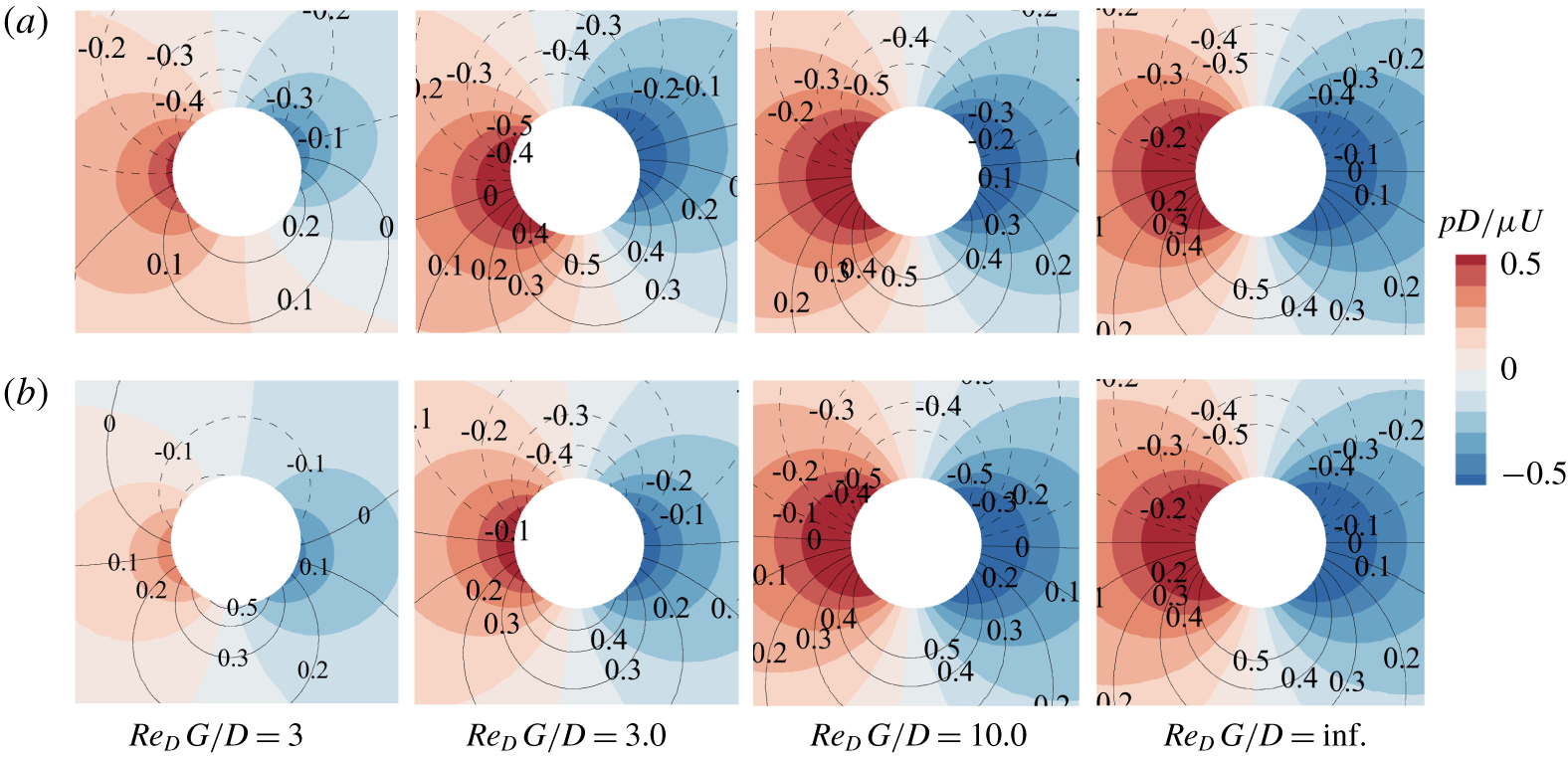
Pressure and vorticity contours around (a) first bristle and (b) fifth bristle of the five-bristle model for  $Re_{D}=0.1$ and
 $\unicode[STIX]{x1D6FC}=45^{\circ }$. The dashed and solid contour lines denote negative and positive vorticities (
 $\unicode[STIX]{x1D714}D/U$), respectively; and
 $Re_{D}\,G/D=\text{inf.}$ indicates the case of a single isolated cylinder.

Spatial distributions of pressure force and viscous force per unit surface area acting on the surface of (a,b) first bristle and (c,d) fifth bristle of the five-bristle model for  $Re_{D}=0.1$ and
 $\unicode[STIX]{x1D6FC}=45^{\circ }$:
 $y$ component of (a,c) pressure force and (b,d) viscous force.

As shown in figure 7, the forces acting on each bristle of the oblique wing model with  $\unicode[STIX]{x1D6FC}<90^{\circ }$ are no longer symmetric with respect to the third bristle in the middle and exhibit different trends from those of the wing model with
 $\unicode[STIX]{x1D6FC}=90^{\circ }$. To determine how changing
 $Re_{D}\,G/D$ affects the flow fields and the surface force distribution for the oblique wing, we examine the representative case of
 $\unicode[STIX]{x1D6FC}=45^{\circ }$ and
 $Re_{D}=0.1$ (figures 8 and 9). Here, we focus on lift because lift can be considered as one of the parameters to determine the aerodynamic performance of the oblique wing and lift changes more notably than drag when we change
 $\unicode[STIX]{x1D6FC}$ from
 $90^{\circ }$ to
 $45^{\circ }$ (figure 7). We choose the two outermost bristles, the first and fifth ones, because they behave differently with regard to lift generation.
For  $Re_{D}\,G/D=3.0$ close to the maximum lift of the first bristle (figure 7d), the
 $y$ components
 $f_{p,y}$ and
 $f_{v,y}$ of the pressure and viscous forces, respectively, change their signs at values of the polar angle
 $\unicode[STIX]{x1D703}$ that are quite different from that of the single isolated bristle,
 $Re_{D}\,G/D=\text{inf.}$ (figure 9a,b). The sign of
 $f_{p,y}$ changes from positive to negative at
 $\unicode[STIX]{x1D703}=108^{\circ }$ and
 $286^{\circ }$, and the sign of
 $f_{v,y}$ changes at
 $\unicode[STIX]{x1D703}=18^{\circ }$ and
 $196^{\circ }$, thereby helping to enlarge the areas of positive
 $f_{p,y}$ and
 $f_{v,y}$ and consequently the overall lift. Interestingly, the polar angle for the change from negative to positive values is unaffected by
 $Re_{D}\,G/D$. Moreover, for
 $Re_{D}\,G/D=3.0$ of the first bristle, the magnitudes of the positive peaks of
 $f_{p,y}$ and
 $f_{v,y}$ are greater than those of their negative peaks, and a huge deviation from the single isolated bristle is observed for the negative peaks, which also results in enhanced lift. The flow around the first bristle is tilted anticlockwise (figure 8a). As mentioned in § 3.1, this tilting corresponds to lift being produced on the bristle. As expected, the tilting is most notable for
 $Re_{D}\,G/D=3.0$, with the tilting angle defined in § 3.1 being the largest,
 $\unicode[STIX]{x1D703}_{t}=16.7^{\circ }$.
For  $f_{p,y}$ and
 $f_{v,y}$ of the first bristle, the shift of the polar angle for sign change and the asymmetric distribution of positive and negative peaks are also prominent at
 $Re_{D}\,G/D=0.3$ (figure 9a,b). In fact, the profiles of
 $f_{p,y}$ and
 $f_{v,y}$ for
 $Re_{D}\,G/D=0.3$ differ more from those of a single isolated bristle than do those for
 $Re_{D}\,G/D=3.0$. The tilting angle is
 $\unicode[STIX]{x1D703}_{t}=12.2^{\circ }$ for
 $Re_{D}\,G/D=0.3$, comparable to
 $\unicode[STIX]{x1D703}_{t}=16.7^{\circ }$ for
 $Re_{D}\,G/D=3$ (figure 8a). However, because of the reduced magnitudes of pressure and vorticity on the surface, the lift for
 $Re_{D}\,G/D=0.3$ is only 0.54 times that for
 $Re_{D}\,G/D=3$. As the effective gap width increases beyond
 $Re_{D}\,G/D=3.0$, the flow fields become more symmetric, and the profiles of
 $f_{p,y}$ and
 $f_{v,y}$ are eventually those for a single isolated bristle.
Meanwhile, the tilting angle  $\unicode[STIX]{x1D703}_{t}$ of the fifth bristle remains negative although its magnitude is small, namely
 $\unicode[STIX]{x1D703}_{t}=-1.0^{\circ }$ for
 $Re_{D}\,G/D=0.3$ and
 $\unicode[STIX]{x1D703}_{t}=-1.5^{\circ }$ for
 $Re_{D}\,G/D=3.0$ (figure 8b). Indeed, because of this negative tilting, the lift is negative in the entire range of
 $Re_{D}\,G/D$ (figure 7d). For
 $Re_{D}\,G/D\geqq 3.0$, the curves of
 $f_{p,y}$ and
 $f_{v,y}$ rarely shift and change their signs at polar angles equivalent to those of the single isolated bristle (figure 9c,d). Only
 $f_{p,y}$ for
 $Re_{D}\,G/D=0.3$ displays the curve shift near
 $\unicode[STIX]{x1D703}=90^{\circ }$. Furthermore, both the positive and negative peak values of
 $f_{p,y}$ and
 $f_{v,y}$ for
 $Re_{D}\,G/D\geqq 3.0$ decrease at a nearly uniform rate from those of the single isolated bristle, thereby leading to low lift (figure 7d). Although the results for the second, third and fourth bristles are not presented here, the trends for these bristles change gradually from those of the first bristle to those of the fifth.
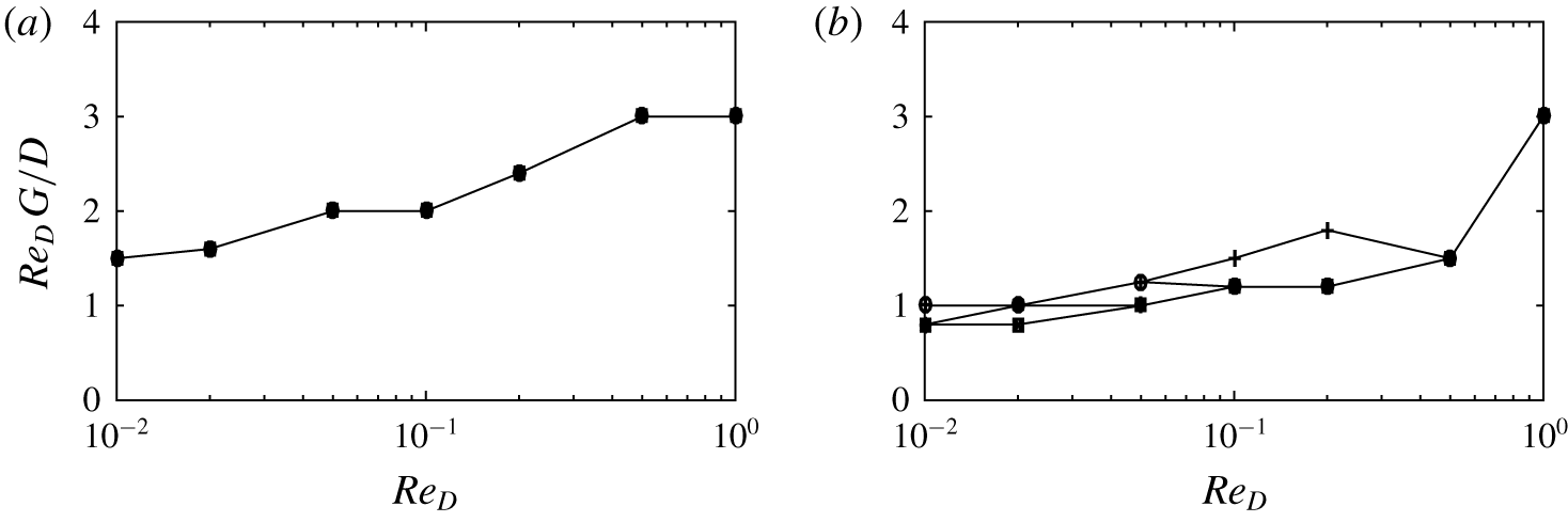
Effective gap width  $Re_{D}\,G/D$ that maximizes (a) lift and (b) lift-to-drag ratio of the entire five-bristle model at a given
 $Re_{D}$. The angle of attack
 $\unicode[STIX]{x1D6FC}$ varies from
 $15^{\circ }$ to
 $75^{\circ }$:
 $\unicode[STIX]{x1D6FC}=15^{\circ }$ (
 $+$),
 $30^{\circ }$ (○),
 $45^{\circ }$ (
 $\ast$),
 $60^{\circ }$ (
 $\times$) and
 $75^{\circ }$ (▫).

As expected, in addition to individual bristles, the variation in the total force for the entire five-bristle model is determined by  $Re_{D}\,G/D$. In the range
 $\unicode[STIX]{x1D6FC}=15^{\circ }$–
 $75^{\circ }$ for the angle of attack, the maximum total lift of the entire wing corresponds to
 $Re_{D}\,G/D=1.5$–3.0, a value that decreases monotonically with a reduction in
 $Re_{D}$ (figure 10a). However, it is notable that the change in
 $Re_{D}\,G/D$ from 1.5 to 3.0 is negligible compared to the 100-fold increment in
 $Re_{D}$ from 0.01 to 1. We conjecture that the optimal value of
 $Re_{D}\,G/D$ leading to the lift peak will converge asymptotically as
 $Re_{D}$ approaches zero. Interestingly, the effective gap width that maximizes the total lift of the entire wing is hardly affected by the change in the angle of attack considered in this study at a given
 $Re_{D}$; the curves for different angles of attack in figure 10(a) are all collapsed. Moreover, the effective gap width that has the maximum lift-to-drag ratio for the entire five-bristle model is also in a narrow range between
 $Re_{D}\,G/D=1.0$ and 3.0 (figure 10b). Similar to the lift presented in figure 10(a), the effect of the angle of attack on determining optimal
 $Re_{D}\,G/D$ for lift-to-drag ratio is insignificant as well, although some variation among different values of
 $\unicode[STIX]{x1D6FC}$ is observed. These intriguing results in figure 10 offer insightful information on how the arrangement of the bristled wing should be adjusted in response to the change in the angle of attack.
3.3 Force estimation for five-bristle model
Perturbed velocity in (a) two-bristle model and (b)  $N$-bristle model, where
 $N$ is the number of bristles. Here
 $\unicode[STIX]{x0394}u_{i}$ and
 $\unicode[STIX]{x0394}v_{i}$ are the
 $x$- and
 $y$-directional velocity perturbations, respectively, at the centre of the dashed bristle as induced by the other bristles.

With the effective gap width introduced, we now estimate the lift and drag acting on the five-bristle model by using a simple theoretical approach that is useful for analysing the optimal configuration of a bristled wing. To explain the principle more simply, we begin by supposing that a bristle (solid circle) is placed alone in a uniform free stream of speed  $U$ (figure 11a). The velocity perturbations induced by this bristle in the
 $x$ and
 $y$ directions are
 $\unicode[STIX]{x0394}u$ and
 $\unicode[STIX]{x0394}v$, respectively, giving a perturbed velocity field
 $u=U+\unicode[STIX]{x0394}u$,
 $v=+\unicode[STIX]{x0394}v$. When a new bristle (dashed circle) is introduced at an arbitrary position, the aerodynamic force applied to the new bristle can be estimated by assuming that the new bristle is subjected to the uniform free stream with
 $u=U+\unicode[STIX]{x0394}u$,
 $v=+\unicode[STIX]{x0394}v$ corresponding to its position because of the linearity of the governing equations of low-Reynolds-number flow (Happel & Brenner Reference Happel and Brenner1983). This assumption is reasonable except when the distance between the bristles is very small. The limitations of this theoretical approach and an alternative force estimation model for narrow gaps are addressed later in this section.
According to Tomotika & Aoi (Reference Tomotika and Aoi1951), the drag force exerted on a single isolated bristle is approximated as
 $$\begin{eqnarray}F=4\unicode[STIX]{x03C0}\unicode[STIX]{x1D707}U\unicode[STIX]{x1D6E5}(Re_{D})=\frac{4\unicode[STIX]{x03C0}\unicode[STIX]{x1D707}U}{[0.5-\unicode[STIX]{x1D6FE}+\ln (8\unicode[STIX]{x1D707}/\unicode[STIX]{x1D70C}UD)]}.\end{eqnarray}$$
Then, in the two-bristle model, the  $x$- and
 $y$-directional forces
 $F_{x}$ and
 $F_{y}$ acting on a bristle (dashed circle in figure 11a) can be computed from (3.5) as
 $$\begin{eqnarray}F_{x}=\frac{4\unicode[STIX]{x03C0}\unicode[STIX]{x1D707}u}{[0.5-\unicode[STIX]{x1D6FE}+\ln (8\unicode[STIX]{x1D707}/\unicode[STIX]{x1D70C}\sqrt{u^{2}+v^{2}}D)]}\quad \text{and}\quad F_{y}=\frac{4\unicode[STIX]{x03C0}\unicode[STIX]{x1D707}v}{[0.5-\unicode[STIX]{x1D6FE}+\ln (8\unicode[STIX]{x1D707}/\unicode[STIX]{x1D70C}\sqrt{u^{2}+v^{2}}D)]}.\end{eqnarray}$$
Instead of the free-stream velocity  $U$, the flow velocity at the position of the bristle, namely
 $u=U+\unicode[STIX]{x0394}u$,
 $v=\unicode[STIX]{x0394}v$, is used in (3.6) to calculate
 $F_{x}$ and
 $F_{y}$;
 $u$ and
 $v$ are obtained from our numerical simulation with a single isolated bristle. The comparisons between the numerical results and theoretically predicted results by (3.6) for the two-bristle model are given in the Appendix.
This theoretical approach used to predict the forces acting on the simple two-bristle model can be extended to the  $N$-bristle model, where
 $N$ is the total number of bristles:
 $N=5$ for the five-bristle model (figure 11b). For the five-bristle model, we assume that the perturbed velocity vector at the location of a new
 $i$th bristle (dashed circle) can be obtained by summing the velocity perturbations from the other four bristles (solid circles):
 $$\begin{eqnarray}u_{i}=U+\mathop{\sum }_{j=1,j\neq i}^{N}\unicode[STIX]{x0394}u_{i,j}\quad \text{and}\quad v_{i}=\mathop{\sum }_{j=1,j\neq i}^{N}\unicode[STIX]{x0394}v_{i,j},\end{eqnarray}$$
where  $\unicode[STIX]{x0394}u_{i,j}$ and
 $\unicode[STIX]{x0394}v_{i,j}$ are the
 $u$- and
 $v$-velocity perturbations at the location of the
 $i$th bristle, which are induced by the
 $j$th bristle. To compute
 $\unicode[STIX]{x0394}u_{i,j}$ and
 $\unicode[STIX]{x0394}v_{i,j}$, we assume that the
 $j$th bristle is placed solely in a uniform flow. In other words, by acquiring the velocity field around a single isolated bristle, the velocity vector
 $[u_{i},v_{i}]$ at any bristle location of the multi-bristle model can be constructed by linear superposition. As mentioned before, we obtain the velocity field around a single isolated bristle from our numerical simulation.
With the velocity vector of (3.7), the lift and drag acting on the  $i$th bristle and the entire five-bristle model can be constructed from (3.6) as
 $$\begin{eqnarray}\displaystyle & \displaystyle F_{x,i}=\frac{4\unicode[STIX]{x03C0}\unicode[STIX]{x1D707}u_{i}}{[0.5-\unicode[STIX]{x1D6FE}+\ln (8\unicode[STIX]{x1D707}/\unicode[STIX]{x1D70C}\sqrt{u_{i}^{2}+v_{i}^{2}}D)]}\quad \!\text{and}\!\quad F_{y,i}=\frac{4\unicode[STIX]{x03C0}\unicode[STIX]{x1D707}v_{i}}{[0.5-\unicode[STIX]{x1D6FE}+\ln (8\unicode[STIX]{x1D707}/\unicode[STIX]{x1D70C}\sqrt{u_{i}^{2}+v_{i}^{2}}D)]}, & \displaystyle \nonumber\\ \displaystyle & & \displaystyle\end{eqnarray}$$
 $$\begin{eqnarray}\displaystyle & \displaystyle F_{x,tot}=\mathop{\sum }_{i=1}^{N}F_{x,i}\quad \text{and}\quad F_{y,tot}=\mathop{\sum }_{i=1}^{N}F_{y,i}. & \displaystyle\end{eqnarray}$$
 $[Re_{D},\unicode[STIX]{x1D6FC}]=[0.1,45^{\circ }]$ and
 $[0.1,15^{\circ }]$. Interestingly, the theoretical estimations of lift and drag forces by (3.8) are in excellent agreement with the numerical results for high
 $Re_{D}\,G/D$, and the discrepancy between them becomes more significant at low
 $Re_{D}\,G/D$. This is because the aerodynamic coupling between the bristles is more prevalent and simple linear superposition is no longer valid in the range of small
 $Re_{D}\,G/D$ (figure 12). Here, we mean proximity in the context of aerodynamic interaction rather than the physical distance
 $G/D$;
 $Re_{D}\,G/D$ is a more relevant parameter than
 $G/D$.
Comparison between total drag  $F_{x,tot}^{\ast }$ and total lift
 $F_{y,tot}^{\ast }$ estimated by (3.8) (red curve) and by the flat-wing model of (3.9) (blue curve) and those obtained by numerical simulation (black curve) for the entire five-bristle model at
 $Re_{D}=0.1$: (a,b)
 $\unicode[STIX]{x1D6FC}=45^{\circ }$; and (c,d)
 $\unicode[STIX]{x1D6FC}=15^{\circ }$. Here
 $F_{x,tot}$ and
 $F_{y,tot}$ are normalized by the drag force
 $F_{x,s}$ of a single isolated bristle with free-stream velocity
 $U$. (e) Schematic diagrams of a bristled wing and a corresponding flat plate with identical length.

The difference between the theoretical estimate and the numerical result is notable for  $F_{x}^{\ast }$ of
 $\unicode[STIX]{x1D6FC}=15^{\circ }$ even at large
 $Re_{D}\,G/D$ (figure 12c). At low angle of attack, the bristles behind the first one are not exposed fully to the free stream. Consequently, the basic assumption used in (3.7) that the
 $x$ velocity is simply the sum of the free-stream velocity and the perturbed
 $x$ velocities due to the other bristles is far from acceptable. In contrast to
 $F_{x}^{\ast }$, the prediction of (3.8) is quite accurate for
 $F_{y}^{\ast }$ at large
 $Re_{D}\,G/D$ (figure 12d), which means that the
 $v$-velocity perturbations are less affected by the insufficient exposure to the free stream than are the
 $u$-velocity perturbations.
When  $Re_{D}\,G/D$ is small, strong virtual fluid barriers form in the gaps among the bristles to hinder the flow from penetrating the gaps, and the bristle model behaves aerodynamically like a flat wing with no gaps. Therefore, for small
 $Re_{D}\,G/D$, we can estimate the force on the five-bristle model by replacing it with a flat plate rather than relying on the inaccurate approach of (3.8) (figure 12e). If the Reynolds number is small, the drag and lift coefficients of the flat plate can be expressed analytically (Imai Reference Imai1954) as
 $$\begin{eqnarray}\displaystyle C_{d} & = & \displaystyle \frac{16\unicode[STIX]{x03C0}}{Re_{L}}\frac{2S-1-\cos 2\unicode[STIX]{x1D6FC}}{G}-\frac{\unicode[STIX]{x03C0}Re_{L}}{4G}\left[S^{2}+\frac{1}{2}(1-2\cos 2\unicode[STIX]{x1D6FC}-\cos 4\unicode[STIX]{x1D6FC})S\right.\nonumber\\ \displaystyle & & \displaystyle -\,\frac{1}{24}(9+8\cos 2\unicode[STIX]{x1D6FC}-7\cos 4\unicode[STIX]{x1D6FC})\nonumber\\ \displaystyle & & \displaystyle +\,\frac{1}{G}\left(\frac{1}{12}(30+23\cos 2\unicode[STIX]{x1D6FC}-10\cos 4\unicode[STIX]{x1D6FC}-3\cos 6\unicode[STIX]{x1D6FC})S\right.\nonumber\\ \displaystyle & & \displaystyle -\!\left.\left.\frac{1}{12}(14+21\cos 2\unicode[STIX]{x1D6FC}+6\cos 4\unicode[STIX]{x1D6FC}-\cos 6\unicode[STIX]{x1D6FC})\right)\right],\end{eqnarray}$$
 $$\begin{eqnarray}\displaystyle C_{l} & = & \displaystyle \frac{16\unicode[STIX]{x03C0}}{Re_{L}}\frac{\sin 2\unicode[STIX]{x1D6FC}}{G}\left\{1-\frac{Re_{L}^{2}}{64}\left[2S^{2}+(1+\cos 2\unicode[STIX]{x1D6FC})S+\frac{1}{3}(2-\cos 2\unicode[STIX]{x1D6FC})\right.\right.\nonumber\\ \displaystyle & & \displaystyle \times \!\left.\left.\frac{1}{G}\left(\frac{1}{2}(5+4\cos 2\unicode[STIX]{x1D6FC}+\cos 4\unicode[STIX]{x1D6FC})S+\frac{1}{3}(9+10\cos 2\unicode[STIX]{x1D6FC}+\cos 4\unicode[STIX]{x1D6FC})\right)\right]\right\},\end{eqnarray}$$
 $Re_{L}=UL/\unicode[STIX]{x1D708}$ is based on the length of the flat plate,
 $G=4S^{2}-2(1+\cos 2\unicode[STIX]{x1D6FC})$,
 $S=\ln (16/Re_{L})-\unicode[STIX]{x1D6FE}$ and
 $\unicode[STIX]{x1D6FE}=0.5772$ is Euler’s constant. If (3.9) is used to predict the forces on the bristled wing at low
 $Re_{D}\,G/D$, then
 $L$ of (3.9) is assumed to be equivalent to the distance between the centres of the first and fifth bristles (figure 12e). Then, to acquire
 $F_{x,tot}^{\ast }$ and
 $F_{y,tot}^{\ast }$, the forces
 $F_{x,tot}=C_{d}\unicode[STIX]{x1D70C}U^{2}L/2$ and
 $F_{y,tot}=C_{l}\unicode[STIX]{x1D70C}U^{2}L/2$ on the flat plate are normalized by the drag
 $F_{x,s}$ on a single isolated bristle of diameter
 $D$.
Because (3.9) is applicable to  $Re_{L}<2$ (Imai Reference Imai1954), the force obtained by our flat-plate model of (3.9) is valid for
 $Re_{D}\,G/D<0.5$ because
 $Re_{D}\,G/D=Re_{L}/4$. For this reason, we plot the curve in figure 12 for
 $Re_{D}\,G/D$ between 0 and 0.5 only. In this
 $Re_{D}\,G/D$ range, the forces predicted by the flat-plate model (blue curve) agree well with the actual forces of the five-bristle model (black curve). However, the deviation between them tends to grow with
 $Re_{D}\,G/D$. In summary, the flat-plate model (3.9) for small
 $Re_{D}\,G/D$ and (3.8) for large
 $Re_{D}\,G/D$ suggest good estimation of both drag and lift. In figure 12(b) for
 $F_{y,tot}$ at
 $\unicode[STIX]{x1D6FC}=45^{\circ }$, the flat-plate model and (3.8) exhibit the accuracy of predictions within 35 % and 13 % for
 $Re_{D}\,G/D<0.5$ and
 $Re_{D}\,G/D>3.0$, respectively. The accuracies of both models to predict
 $F_{y,tot}$ improve for
 $\unicode[STIX]{x1D6FC}=15^{\circ }$ (figure 12d), and the differences are reduced to 22 % and 4 %, respectively. Admittedly, both theoretical models have limited accuracy when estimating the maximum lift, but they allow us to approximate the range of
 $Re_{D}\,G/D$ in which maximum lift should arise. In addition to
 $Re_{D}=0.1$, although not reported in figure 12, we confirmed that the aforementioned trends of the forces predicted by the two models pertained also to
 $Re_{D}=0.01$.
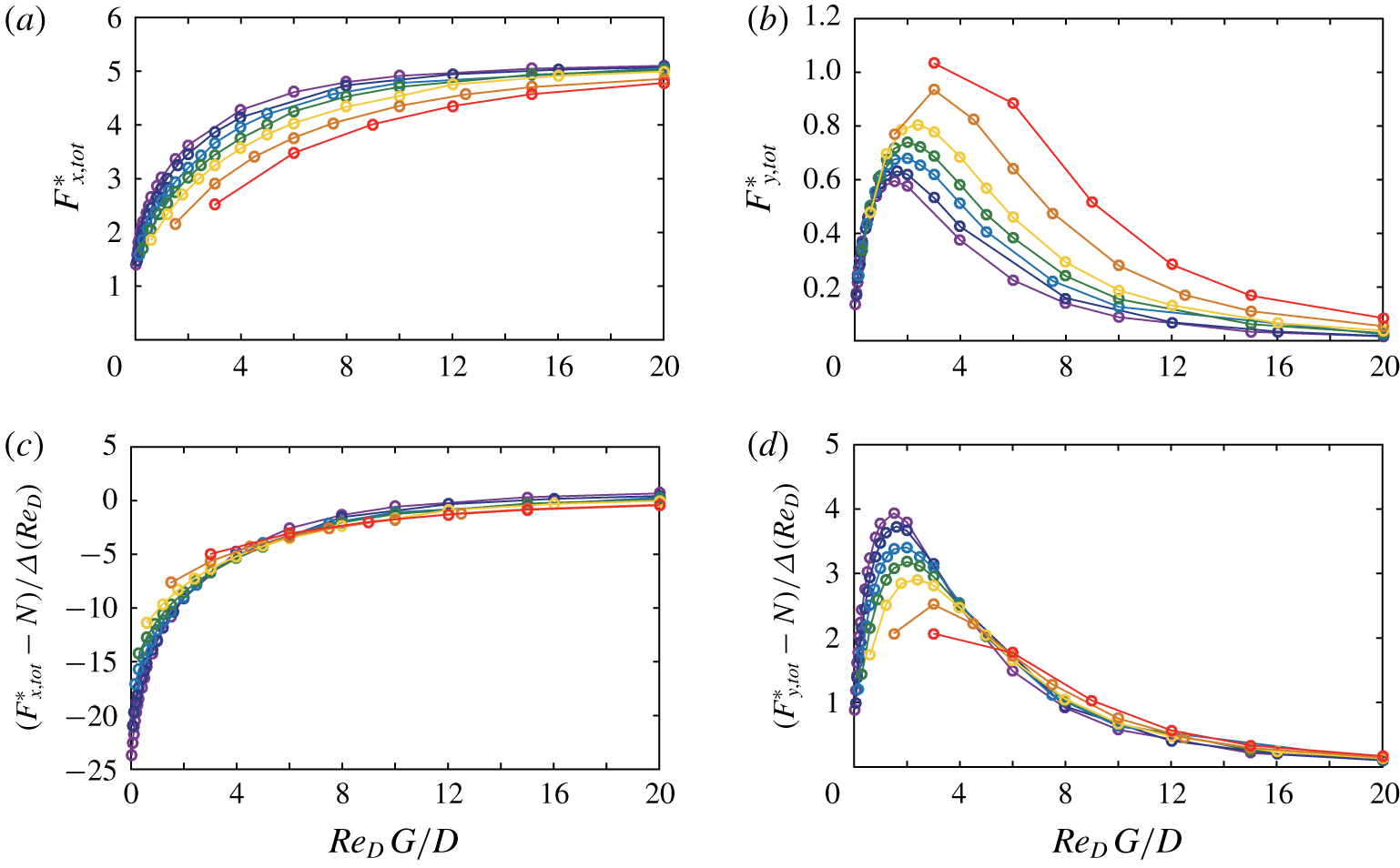
(a,b) Total drag  $F_{x,tot}^{\ast }$ and total lift
 $F_{y,tot}^{\ast }$ obtained by numerical simulations for the entire five-bristle model at
 $\unicode[STIX]{x1D6FC}=45^{\circ }$. (c,d) Plots of
 $F_{x,tot}^{\ast }$ and
 $F_{y,tot}^{\ast }$ normalized by
 $\unicode[STIX]{x1D6E5}(Re_{D})=(\text{ln}(8/Re_{D})-\unicode[STIX]{x1D6FE}+0.5)^{-1}$. The plots are for
 $Re_{D}=1$ (red), 0.2 (orange), 0.5 (yellow), 0.1 (green), 0.05 (blue), 0.02 (navy) and 0.01 (purple).

Thus far, we have presented  $F_{x,tot}^{\ast }$ and
 $F_{y,tot}^{\ast }$ of the entire wing as functions of the effective gap width
 $Re_{D}\,G/D$. As discussed in § 3.2, the introduction of
 $Re_{D}\,G/D$ is motivated by the scaled
 $y$ coordinate
 $Re_{D}\,y/D$ shown in figure 5. According to (3.4), there exists the Reynolds-number-dependent constant
 $\unicode[STIX]{x1D6E5}(Re_{D})$ in the leading term of the velocity disturbance. Then, in figure 5, the perturbed velocity is normalized by
 $\unicode[STIX]{x1D6E5}(Re_{D})$ to better predict its trend. In a similar way, we provide
 $F_{x,tot}^{\ast }$ and
 $F_{y,tot}^{\ast }$ normalized by
 $\unicode[STIX]{x1D6E5}(Re_{D})$ in figure 13(c,d), namely
 $$\begin{eqnarray}\frac{F_{x,tot}^{\ast }-N}{\unicode[STIX]{x1D6E5}(Re_{D})}\left(=\mathop{\sum }_{i=1}^{N}\frac{F_{x,i}-F_{x,s}}{F_{x,s}\unicode[STIX]{x1D6E5}(Re_{D})}\right)\quad \text{and}\quad \frac{F_{y,tot}^{\ast }}{\unicode[STIX]{x1D6E5}Re_{D}}.\end{eqnarray}$$
While  $F_{x,tot}^{\ast }$ and
 $F_{y,tot}^{\ast }$ in figure 13(a,b) show relatively large variations between the curves for different values of
 $Re_{D}$, the curves in figure 13(c,d) greatly diminish such variation and tend to collapse together, in particular for
 $Re_{D}\,G/D>5$. For instance, at
 $Re_{D}\,G/D=6$ and
 $\unicode[STIX]{x1D6FC}=45^{\circ }$,
 $F_{y,tot}^{\ast }$ for
 $Re_{D}=1$ is roughly four times greater than that for
 $Re_{D}=0.01$ (figure 13b). However, the difference in
 $F_{y,tot}^{\ast }/\unicode[STIX]{x1D6E5}(Re_{D})$ between
 $Re_{D}=1$ and
 $Re_{D}=0.01$ lies within 20 % under the same conditions (figure 13d). The results in figure 13(c,d) imply that the force normalized by
 $\unicode[STIX]{x1D6E5}(Re_{D})$ better characterizes the force trend expressed as a function of
 $Re_{D}\,G/D$.
3.4 Force estimation for 25-bristle model
The theoretical approaches that we introduced with the five-bristle model can be extended to the model composed of a larger number of bristles. To demonstrate that our findings can be applied generally to a 2-D bristled wing with any number of bristles, a 25-bristle model will be considered here as a representative case. The 25 bristles of diameter  $D$ are equally spaced in a straight line (figure 1b). For the 25-bristle model, the Reynolds number
 $Re_{D}$ ranges from 0.01 to 1.0, i.e.
 $Re_{D}=[0.01,0.02,0.05,0.1,0.2,0.5,1.0]$, but the angle of attack,
 $\unicode[STIX]{x1D6FC}$, is fixed to be
 $45^{\circ }$.
(a,b) Total drag  $F_{x,tot}^{\ast }$ and total lift
 $F_{y,tot}^{\ast }$ obtained by numerical simulations for the entire 25-bristle model at
 $\unicode[STIX]{x1D6FC}=45^{\circ }$. (c,d) Plots of
 $F_{x,tot}^{\ast }$ and
 $F_{y,tot}^{\ast }$ normalized by
 $\unicode[STIX]{x1D6E5}(Re_{D})=(\text{ln}(8/Re_{D})-\unicode[STIX]{x1D6FE}+0.5)^{-1}$. The plots are for
 $Re_{D}=1$ (red), 0.2 (orange), 0.5 (yellow), 0.1 (green), 0.05 (blue), 0.02 (navy) and 0.01 (purple).

In a similar way to figure 13, we present  $F_{x,tot}^{\ast }$ and
 $F_{y,tot}^{\ast }$ of the entire 25-bristle model as functions of the effective gap width
 $Re_{D}\,G/D$ (figure 14a,b). In common with the five-bristle model, the aerodynamic performances are successfully characterized by
 $Re_{D}\,G/D$. With
 $Re_{D}\,G/D$, the curves of
 $F_{x,tot}^{\ast }$ show a consistent pattern, and converge towards 25 (figure 14a). Regardless of the Reynolds number based on
 $D$ (
 $Re_{D}$),
 $F_{x,tot}^{\ast }$ of each curve is greater than 20 near
 $Re_{D}\,G/D>12$. The total lift has a peak in a narrow range of
 $Re_{D}\,G/D$ between 1.5 and 6.0, which is similar to the five-bristle model (figure 14b). Interestingly, the value of
 $Re_{D}\,G/D$ corresponding to the peak of the lift is hardly affected by the number of bristles (i.e. five or 25) for
 $Re_{D}$ below 0.1. Also,
 $F_{x,tot}^{\ast }$ and
 $F_{y,tot}^{\ast }$ normalized by
 $\unicode[STIX]{x1D6E5}(Re_{D})$ are provided for the 25-bristle model (figure 14c,d); also see (3.10). Similar to the five-bristle model, the deviations between the curves of different
 $Re_{D}$ values diminish for
 $Re_{D}\,G/D>6$.
In addition to the characterization of the force trends with  $Re_{D}\,G/D$ and
 $\unicode[STIX]{x1D6E5}(Re_{D})$, we will show that the theoretical approach used to predict the forces acting on the five-bristle model (figure 11b) can be extended to the 25-bristle model. The perturbed velocity vector at the location of a new
 $i$th bristle can be obtained by summing the velocity perturbations from the other 24 bristles as shown in (3.7):
 $N=25$. With the velocity components in (3.7), the lift and drag acting on the
 $i$th bristle and the entire 25-bristle model can be constructed from (3.8).
Comparison between (a) total drag  $F_{x,tot}^{\ast }$ and (b) total lift
 $F_{y,tot}^{\ast }$ estimated by (3.8) (red curve) and by the flat-wing model of In, Choi & Kim (Reference In, Choi and Kim1995) (blue curve) and those obtained by numerical simulation (black curve) for the entire 25-bristle model at
 $Re_{D}=0.1$ and
 $\unicode[STIX]{x1D6FC}=45^{\circ }$. Here
 $F_{x,tot}$ and
 $F_{y,tot}$ are normalized by the drag force
 $F_{x,s}$ of a single isolated bristle with free-stream velocity
 $U$. The flat-wing model has the same length as the corresponding bristled wing.

The total forces evaluated by (3.8) are shown in figure 15 for one representative case of  $Re_{D}=0.1$. Similar to the five-bristle model (figure 12), the theoretical estimate of (3.8) matches well with the numerical result for high
 $Re_{D}\,G/D$, and the discrepancy between them becomes greater at low
 $Re_{D}\,G/D$. For low
 $Re_{D}\,G/D$, the simple linear superposition breaks down, and instead the flat-plate model can be considered to estimate the forces. The Reynolds number based on the length of the flat plate,
 $Re_{L}~(=UL/\unicode[STIX]{x1D708})$, is much greater than unity even for the smallest
 $Re_{D}\,G/D~(=0.3)$ considered in figure 15:
 $Re_{L}=24Re_{D}\,G/D\geqslant 7.2$. Therefore, numerically computed forces by In et al. (Reference In, Choi and Kim1995) were used for the flat-wing model (blue curves in figure 15). In summary, the flat-plate model for small
 $Re_{D}\,G/D$ and (3.8) for large
 $Re_{D}\,G/D$ suggest good estimation for both drag and lift. Note that both flat-plate model and (3.8) are valid in almost the same ranges of
 $Re_{D}\,G/D$ as those of the five-bristle model (figures 12 and 15). Because of the linear property of the Oseen equation for the flow around the bristled wing, similar trends in force generation are observed regardless of the number of bristles.
4 Concluding remarks
For a bristled-wing model in 2-D low-Reynolds-number flow, we have investigated aerodynamic force generation and its correlation with flow fields in wide ranges of the Reynolds number ( $Re_{D}=0.01$–1) and gap width (
 $G/D=3$–2000). By noting that the Reynolds number and gap width have similar effects on the formation of virtual fluid barriers and the variations of the drag and lift forces exerted on the wing, the effective gap width
 $Re_{D}\,G/D$ that couples the Reynolds number and the gap width aerodynamically is introduced to characterize the collective interaction of multiple bristles in low-Reynolds-number flow. As the Reynolds number decreases below
 $Re_{D}=1$, the aerodynamic characterization by the effective gap width
 $Re_{D}\,G/D$ is better suited because the flow asymptotically converges to the very-low-Reynolds number solution, where the Reynolds number based on
 $G$ (
 $Re_{G}=Re_{D}\,G/D$) is the governing parameter. In addition, the scaled force ratio that explicitly includes the Reynolds number is introduced as a new measure of aerodynamic performance. For the five-bristle model, for all Reynolds numbers considered, the total drag normalized by
 $\unicode[STIX]{x1D6E5}(Re_{D})=(\text{ln}(8/Re_{D})-\unicode[STIX]{x1D6FE}+0.5)^{-1}$ acting on the entire model increases with the effective gap width and converges near
 $Re_{D}\,G/D=6$, and the total lift normalized by
 $\unicode[STIX]{x1D6E5}(Re_{D})=(\text{ln}(8/Re_{D})-\unicode[STIX]{x1D6FE}+0.5)^{-1}$ has a peak in a narrow range of
 $Re_{D}\,G/D$ between 1.5 and 3. The notable trends of the forces in terms of the effective gap width are accounted for by the asymmetric spatial distribution of the forces induced by pressure and viscous stress on the surface of each bristle and the tilting of the pressure and vorticity fields around each bristle.
The drag and lift forces can be predicted theoretically with good accuracy by using the linear superposition of velocity vectors around a single isolated bristle for large  $Re_{D}\,G/D$ and by adopting the alternative flat-plate model for small
 $Re_{D}\,G/D$. By virtue of the linearity of the governing equations of low-Reynolds-number flow, we can extend the same theoretical approaches for the five-bristle model to the model with the larger number of bristles (e.g. 25-bristle model).
As a fundamental study to obtain insights into how to optimize a bristled wing, our intention herein was to limit our target model to a simple wing with equally spaced identical bristles in a straight line in a 2-D fluid domain instead of considering the actual bristled-wing designs of the smallest insects. Based on the findings and analytical approaches of the present study, in future work we will extend our study to explore the strategies of aerodynamic optimization for more complex configurations such as unequally spaced bristles, cambered bristled wings and ultimately 3-D bristled wings.
Acknowledgements
This research was supported by the Basic Science Research Program through the National Research Foundation of Korea (NRF) funded by the Ministry of Science and ICT (NRF-2017R1E1A1A01074704), and by a grant (KCG-01-2016-04) through the Korea Institute of Marine Science and Technology funded by Korea Coast Guard of Korea government.
Declaration of interests
The authors report no conflict of interest.
Appendix. Two-bristle model
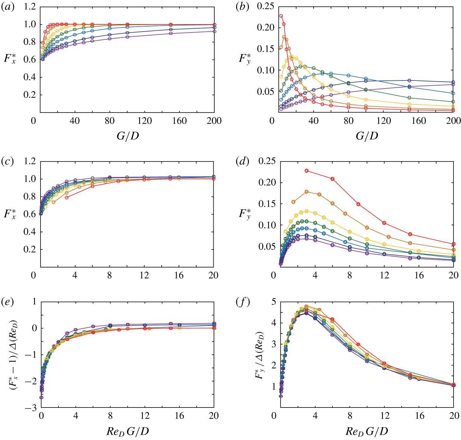
Through § 3, we discussed our results for five- and 25-bristle models. The two-bristle model is the simplest model to confirm whether the characteristics of the creeping flow around a single isolated bristle can be extended to multi-bristle configurations. In fact, before obtaining the results for five- and 25-bristle models, we preliminarily examined the two-bristle model in which two bristles are arranged side-by-side, normal to the free stream ( $\unicode[STIX]{x1D6FC}=90^{\circ }$). The results for the two-bristle model are briefly presented in figure 16.
The drag  $F_{x}^{\ast }$ and lift
 $F_{y}^{\ast }$ forces on the upper bristle of the two-bristle model are better characterized by the effective gap width
 $Re_{D}\,G/D$, rather than by the gap width ratio
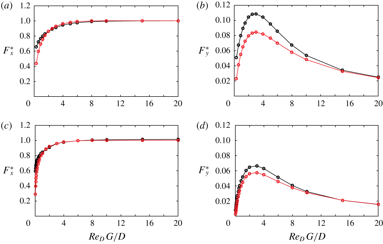
 $G/D$ (figure 16a–d), similar to the five- and 25-bristle models (figures 13a,b and 14a,b). The
 $F_{x}^{\ast }$ value converges near
 $Re_{D}\,G/D=6$, and
 $F_{y}^{\ast }$ has a peak in a narrow range of
 $Re_{D}\,G/D$ around 3. In addition,
 $F_{x}^{\ast }$ and
 $F_{y}^{\ast }$ normalized by
 $\unicode[STIX]{x1D6E5}(Re_{D})$ collapse together regardless of the values of
 $Re_{D}$ (figure 16e,f). The same trend is reported for the five- and 25-bristle models with minor variation between curves around
 $Re_{D}\,G/D<5$ (figures 13a,b and 14a,b).
The numerical results and theoretically predicted results for the two-bristle model at  $\unicode[STIX]{x1D6FC}=90^{\circ }$ are compared in figure 17. As discussed in §§ 3.3 and 3.4, the forces theoretically estimated by (3.8) are in excellent agreement with the numerically calculated forces for the large effective gap width
 $Re_{D}\,G/D$ (figure 17). The assumption used to derive (3.8) is not valid when the bristles are very close to each other, because the perturbation induced by a bristle becomes significant. Indeed, for small
 $Re_{D}\,G/D$, relatively large discrepancy is observed between the theoretical prediction and the numerical result. The difference in
 $F_{x}^{\ast }$ becomes notable at
 $Re_{D}\,G/D<1$. Meanwhile,
 $F_{y}^{\ast }$ shows greater discrepancy than does
 $F_{x}^{\ast }$ in the broader range of
 $Re_{D}\,G/D$, and the peak of
 $F_{y}^{\ast }$ presents an error of roughly 20 % from the numerical result. Given that the magnitude of
 $F_{y}^{\ast }$ is one order smaller than that of
 $F_{x}^{\ast }$ in figure 17, note that the prediction of
 $F_{y}^{\ast }$ is also good if the order of magnitude is considered.
(a,b) Drag  $F_{x}^{\ast }$ and lift
 $F_{y}^{\ast }$ forces of the upper bristle in two-bristle model at
 $\unicode[STIX]{x1D6FC}=90^{\circ }$; (c,d)
 $F_{x}^{\ast }$ and
 $F_{y}^{\ast }$ replotted with effective gap width
 $Re_{D}\,G/D$; and (e,f)
 $F_{x}^{\ast }$ and
 $F_{y}^{\ast }$ normalized by
 $\unicode[STIX]{x1D6E5}(Re_{D})=(\text{ln}(8/Re_{D})-\unicode[STIX]{x1D6FE}+0.5)^{-1}$. The plots are for
 $Re_{D}=1$ (red), 0.2 (orange), 0.5 (yellow), 0.1 (green), 0.05 (blue), 0.02 (navy) and 0.01 (purple).

Comparison between drag and lift forces estimated by (3.6) (red curve) and those obtained by numerical simulation (black curve) for the upper bristle of the two-bristle model at  $\unicode[STIX]{x1D6FC}=90^{\circ }$: (a,b)
 $Re_{D}=0.1$; and (c,d)
 $Re_{D}=0.01$. The forces are normalized by the drag force
 $F_{x,s}$ of a single isolated bristle with free-stream velocity
 $U$; see (3.1).

The numerical results and theoretically predicted results in figure 17 show the better agreement for  $Re_{D}=0.01$, compared to
 $Re_{D}=0.1$, because of the stronger linearity of the flow field and force. For both
 $Re_{D}=0.1$ and 0.01, the drag curves of the numerical simulation and theoretical prediction begin to differ as
 $Re_{D}\,G/D$ approaches zero. However, a notable discrepancy begins to occur at smaller
 $Re_{D}\,G/D$ for
 $Re_{D}=0.01$, compared to
 $Re_{D}=0.1$ (figure 17a,c). At
 $Re_{D}\,G/D=0.3$, for example, the numerically computed value of
 $F_{x}^{\ast }$ is 1.50 times greater than that of the theoretically predicted value for
 $Re_{D}=0.1$. Meanwhile, for
 $Re_{D}=0.01$, the numerical value of
 $F_{x}^{\ast }$ is only 1.15 times the theoretical value. Similar trends are also observed in the curves of
 $F_{y}^{\ast }$ (figure 17b,d).