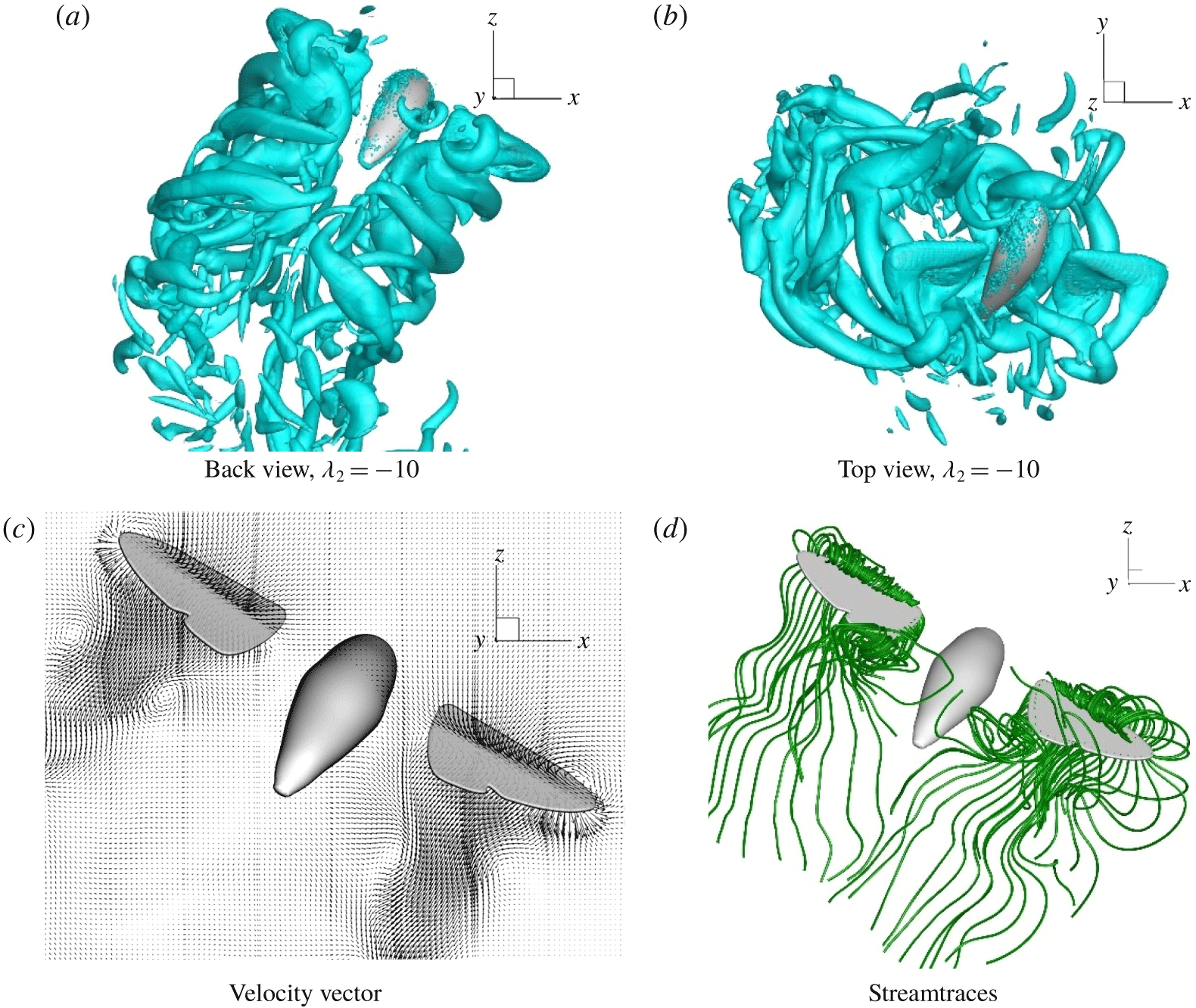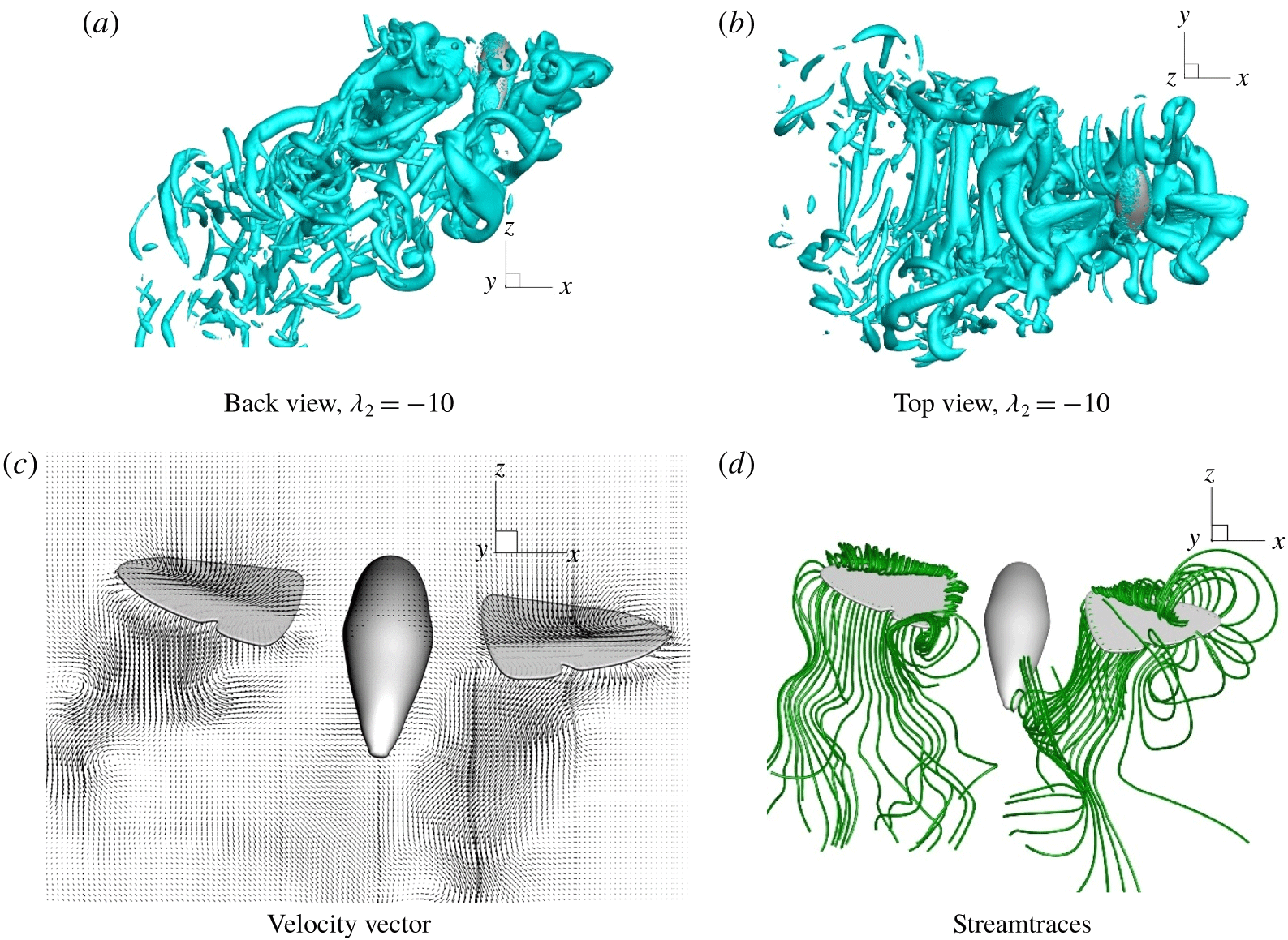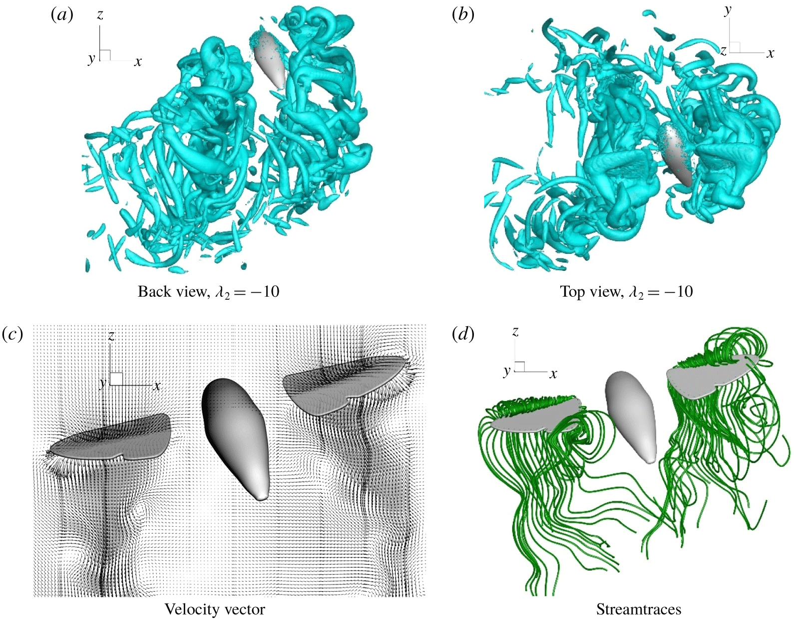


1 Introduction
Insects show superior versatility and manoeuvrability among flying animals that have developed a set of flying skills to access the abundant ecological resources or to escape rapidly from predators. Great efforts have been made by researchers to unravel the physical phenomena underlying the fascinating flight performance of insects over the past decades. Flapping-wing flight appears to be more advantageous in terms of its manoeuvrability and efficiency compared with conventional fixed-wing mode, especially in the dynamic range of Reynolds number between 1 and  $10^{4}$ applicable to insects (Shyy et al. Reference Shyy, Lian, Tang, Viieru and Liu2007, Reference Shyy, Aono, Kang and Liu2013; Greeter & Hedrick Reference Greeter and Hedrick2016). Interest in insect aerodynamics has also been motivated by its potential applications in the design of micro air vehicles (MAVs).
The early studies of flapping-wing aerodynamics attempted to estimate the forces generated by the wings using quasi-steady aerodynamics (Osborne Reference Osborne1951; Weis-Fogh & Jensen Reference Weis-Fogh and Jensen1956; Weis-Fogh Reference Weis-Fogh1972, Reference Weis-Fogh1973; Ellington Reference Ellington1984a). The researchers found that conventional aerodynamics had tended to underestimate the actual lift. Since then, several unsteady aerodynamic mechanisms of lift generation have been uncovered and investigated, including but not limited to the leading-edge vortex (Ellington et al. Reference Ellington, Van Den Berg, Willmott and Thomas1996; Birch & Dickinson Reference Birch and Dickinson2001; Srygley & Thomas Reference Srygley and Thomas2002; Houghton & Carpenter Reference Houghton and Carpenter2003; Birch, Dickson & Dickinson Reference Birch, Dickson and Dickinson2004), clap-and-fling mechanism (Weis-Fogh Reference Weis-Fogh1973; Cooter & Baker Reference Cooter and Baker1977; Wootton & Newman Reference Wootton and Newman1979) and wake capturing (Dickinson Reference Dickinson1994; Dickinson, Lehmann & Sane Reference Dickinson, Lehmann and Sane1999; Tang, Viieru & Shyy Reference Tang, Viieru and Shyy2008), etc. These mechanisms may work singly or in unison for the insect flapping wings to produce high transient lift. The flapping-wing kinematics of selected insects have been successfully measured, and their role in force generation clarified, by Willmott & Ellington (Reference Willmott and Ellington1997a,Reference Willmott and Ellingtonb), Dickinson et al. (Reference Dickinson, Lehmann and Sane1999), Fry, Sayaman & Dickinson (Reference Fry, Sayaman and Dickinson2003), Muijres et al. (Reference Muijres, Johansson, Barfield, Wolf, Spedding and Hedenström2008) and others. Computational fluid dynamics (CFD) has advanced rapidly over the past several decades, benefiting from the continuous development in computing hardware and numerical techniques. CFD today arguably offers a complementary and sometimes more expedient approach to study the unsteady aerodynamics at the scales of the insects, revealing details that may be difficult to access experimentally. Numerically focused work on flapping-wing aerodynamics has been carried out by Liu et al. (Reference Liu, Ellington, Kawachi, Van Den Berg and Willmott1998), Wang (Reference Wang2000), Ramamurti & Sandberg (Reference Ramamurti and Sandberg2002), Sun & Tang (Reference Sun and Tang2002), Gilmanov & Sotiropoulos (Reference Gilmanov and Sotiropoulos2005), Miller & Peskin (Reference Miller and Peskin2005, Reference Miller and Peskin2009), Aono, Liang & Liu (Reference Aono, Liang and Liu2008), Liu (Reference Liu2009), Nguyen et al. (Reference Nguyen, Sundar, Yeo and Lim2016) and others. These studies have captured important features of flow and details of force production during the different stages of wing motion for a wide range of Reynolds number.
Insect flight is fundamentally an unconstrained dynamic state in three-dimensional (3-D) space, where the adequacy of aerodynamic lift is only a minimum necessary condition. In more recent times, researchers have begun to turn their attention to free flight wherein the interactions between insect motion and aerodynamic flow play a leading role. Taylor & Thomas (Reference Taylor and Thomas2003) surmised that an insect’s static stability and static control responses are insufficient to provide asymptotic longitudinal dynamic stability. Sun & Xiong (Reference Sun and Xiong2005), Sun, Wang & Xiong (Reference Sun, Wang and Xiong2007) and Xiong & Sun (Reference Xiong and Sun2008) investigated the longitudinal dynamic stability of four insects in hovering and forward flight and showed that the longitudinal motion of the insects at all flight speeds is dynamically unstable because of one or two unstable modes. Wu, Zhang & Sun (Reference Wu, Zhang and Sun2009) and Wu & Sun (Reference Wu and Sun2012) showed that the periodic state of reciprocating wing insect flight is unstable, while Zhang & Sun (Reference Zhang and Sun2010) showed that the lateral motion of the dronefly is also unstable because of an unstable divergence mode. Hedrick & Daniel (Reference Hedrick and Daniel2006), on the other hand, using a micro-genetic selection algorithm, showed that a hawkmoth could free hover via a multitude of admissible wing kinematics – thus implying that insect flyers do possess considerable latitude in the choice of kinematics to achieve a given flight duty. These studies offer ample evidence that insect flapping-wing flight is inherently unstable, and that insects would need to actively vary their wing kinematics to stay in flight.
More recently, Wu, Yeo & Lim (Reference Wu, Yeo and Lim2014) simulated the free hovering flight of a model fruit fly Drosophila melanogaster, and investigated the real-time dynamics. They argued heuristically that the passive stability of equilibrium hovering states is inherently weak in the mean against pitching divergence, and that active control of the wing kinematics could restore flight stability. Their results showed good consistency and agreement with available flight data of the natural flyer, and verified that insect-type hovering flight could be stabilized by active control based on cycle-averaged kinematic data. Yao & Yeo (Reference Yao and Yeo2018) subsequently extended the hovering model of Wu et al. (Reference Wu, Yeo and Lim2014) to study the forward and reverse longitudinal free flight of the model fruit fly. They were able to sustain stable quasi-steady free flight at different speeds and provided a comprehensive picture of the coupled dynamics of flyer and flow involved in longitudinal free flight.
By and large, the bulk of experimental studies on insect flight have involved flyer subjects that are either tethered or stationary; or else they are assigned prescribed kinematics or motion in the case of CFD simulation. The ‘real-time’ fluid–body coupled dynamic free flight of insects has rarely if ever been explored in detail and reported in the literature. In this paper, we present a detailed numerical and comprehensive study on the aerodynamics of longitudinal free flight and sideslip manoeuvre of a model hummingbird hawkmoth, Macroglossum stellatarum – the first study of its kind for a relatively large insect. As opposed to the diminutive fruit fly ( $Re\sim 150$) studied so far by Wu et al. (Reference Wu, Yeo and Lim2014) and Yao & Yeo (Reference Yao and Yeo2018), the hummingbird hawkmoth is fairly large and heavy among flying insects, and possesses a flapping-wing Reynolds number of
 $Re\sim 3000$. The present study followed the basic framework established by Wu et al. (Reference Wu, Yeo and Lim2014) and Yao & Yeo (Reference Yao and Yeo2018). An important extension was made, however, to the Newtonian model of the flyer in this study to account for the significant reciprocating wing mass of the hawkmoth, together with essential adjustments for simulation at a much higher Reynolds number. The flight dynamics for forward flight and sideslip manoeuvre are also interpreted and analysed in their cycle-mean state-variable form in this work. This is instrumental in helping to identify the roles of the various kinematic actions in the control of flight, motivate strategies of control and facilitate the estimation of the control coefficients that are needed for the ‘real-time’ full-fidelity simulations presented in the paper. The performance of the model insect and underlying physics of aerodynamic force generation (and energetics) are reviewed for all key stages of flight. Leading features of the vortical wake formation are described and their relation to force generation highlighted.
The paper is organized as follows. Section 2 gives the morphological details of the model hawkmoth and describes the geometric and kinematic parameters defining the motion of its body and wings. Section 3 briefly outlines the basic methodology and numerical set-up for the simulation of the coupled fluid–body interaction problem. Section 4 describes the wing kinematic actions and their roles in the control of stable free flights. Section 5 presents the results for the forward flights and a complete sideslip manoeuvre of the model hawkmoth. Section 6 highlights important features of flow associated with the flights and force generation. Section 7 summarizes the key conclusions from the present study.
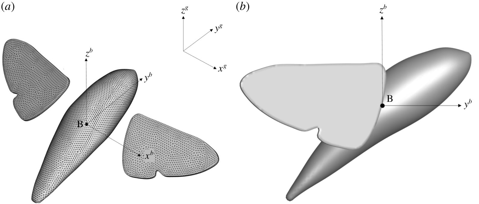
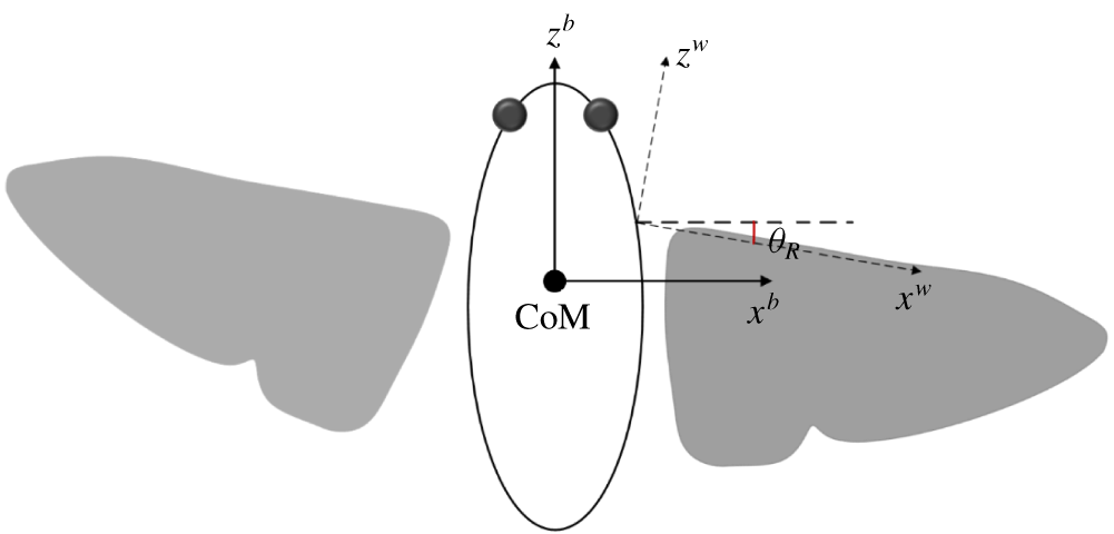
Geometry of insect model and coordinate systems. The longitudinal axis of the insect body is selected as the  $y^{b}$-axis of body frame. The insect model is created with a pre-set pitch angle of
 $45^{\circ }$ in the body frame, which is the approximate body pitching angle during normal hovering flight.

2 Morphological and kinematic model
The hummingbird hawkmoth (M. stellatarum) is adopted as the model flyer in the present work. It is a good representative of the family of Sphingidae, which usually exhibits superior flight performance in terms of aerial agility and manoeuvring versatility among flying insects with relatively high Reynolds number (Greeter & Hedrick Reference Greeter and Hedrick2016). A brief introduction to the morphological and kinematic modelling of the flyer is given in this section; more details may be found in Yao (Reference Yao2018). The flapping-wing motion of the hummingbird hawkmoth has a frequency ( $f$) of approximately 70 Hz and a stroke amplitude (
 $\unicode[STIX]{x1D6F7}$) of approximately
 $115^{\circ }$ according to Wu & Zeng (Reference Wu and Zeng2010). The Reynolds number of the flyer is typically defined with respect to the wing mean chord (
 $\overline{c}$) as the reference length and the average wing-tip velocity (
 $U_{ref}$) as the reference velocity:
 $$\begin{eqnarray}\mathit{Re}={\displaystyle \frac{\overline{c}U_{ref}}{\unicode[STIX]{x1D708}}}={\displaystyle \frac{\overline{c}L2\unicode[STIX]{x1D6F7}f}{\unicode[STIX]{x1D708}}}={\displaystyle \frac{4L^{2}\unicode[STIX]{x1D6F7}f}{\unicode[STIX]{x1D708}\,AR}},\end{eqnarray}$$
where  $\unicode[STIX]{x1D708}=1.5\times 10^{-5}~\text{m}^{2}~\text{s}^{-1}$ is the kinematic viscosity of air,
 $\mathit{AR}=(2L)^{2}/S$ is the aspect ratio of the insect wings and
 $S=2L\overline{c}$ is the surface area of the wing pair. The Reynolds number works out to be approximately 2950.
The present model hawkmoth has a wing length of  $L=20.2~\text{mm}$, and a total mass of 0.2071 g, of which 4.66 % is due to the wings. The geometry of the model hawkmoth was developed from Dickens (Reference Dickens1974) and is shown here in figure 1. The fore and hind wings were treated as a single wing with thickness 2 % of the wing length. The fore and hind wings generally work in unison as a single wing except during highly abrupt manoeuvres, and coupled motion is usually restored in the next stroke (Weis-Fogh Reference Weis-Fogh1973; Willmott & Ellington Reference Willmott and Ellington1997a). They also keep the same relative positional angle and elevation angle during the wing sweeping, with a small difference in their relative twist due to wing flexibility (Liu & Kawachi Reference Liu and Kawachi1998). The single-wing model has been adopted by many other researchers in the study of hawkmoth flight (Aono et al. Reference Aono, Liang and Liu2008; Liu Reference Liu2009; Shyy et al. Reference Shyy, Aono, Chimakurthi, Trizila, Kang, Cesnik and Liu2010; Lua et al. Reference Lua, Lee, Lim and Yeo2016).
The wings were modelled here after the real wings, with a small excision along its inner margin to leave a small gap between the body and the wings. This was done to minimize numerical instabilities arising from the close approach or collision of wings and body during wing flapping. The excised section near the wing root is below 10 % of the total wing area – its geometric centre is very close to the wing root ( ${\sim}0.04$ wing length), and translates at
 ${<}10\,\%$ of the speed of the wing’s geometric centre. Since the wing force produced by the wing motion is proportional to both the wing area and the wing speed, one could surmise that the excised part contributes to
 ${\sim}1\,\%$ of the total wing force. Hence, we do not expect the omission of the excised wing root to have any significant effect on the aerodynamic performance of the wings. Though flexible wings are more efficient in force generation compared with rigid ones, the overall flow structure does not differ much whether the wings are rigid or not (Nakata & Liu Reference Nakata and Liu2012a,Reference Nakata and Liub; Nguyen et al. Reference Nguyen, Sundar, Yeo and Lim2016). As the main focus of the present study concerns the dynamics and aerodynamics of controlled free flight, the model wings were further assumed to be rigid for simplicity. Moreover, detailed mechanical properties and characterization of the real wings are lacking for most insects, due for the most part to their complex physiological construction, comprising a network of interconnected primary and secondary veins of widely varying stiffness with thin connecting membrane (Nguyen et al. Reference Nguyen, Sundar, Yeo and Lim2016). The body model was constructed by neglecting the legs and antennas to avoid unnecessary complexity, since such body features may be expected to have only secondary influence on the aerodynamics.
The complete geometric model is shown by figure 1 in the global coordinate frame  $(x,y,z)^{g}$ and insect-body coordinate frame
 $(x,y,z)^{b}$ (both right-hand systems). The origin of the body frame is at the approximate centre of the body, marked B in figure 1. The origins of the wing frame (not shown in the figure) are attached to two fixed points on the flyer’s body in accordance with the location of the actual wing roots. Free rotation is allowed for the wings about the wing roots to simulate the flapping motion. The insect model was created with a pre-set pitch angle of
 $45^{\circ }$ in the body coordinate frame (figure 1b), which is defined as the reference posture of the insect during flight. The hummingbird hawkmoth pitches approximately at that angle during normal hovering, which is its most fundamental flight mode.
Body motion comprises the displacement of the body centre  $\boldsymbol{X}_{B}(t)=(x,y,z)^{g}(t)$ in the global frame
 $(x,y,z)^{g}$ and the rotation of the body frame relative to the global frame. The rotation is described here by the orientation vector,
 $$\begin{eqnarray}\unicode[STIX]{x1D723}(t)=(\unicode[STIX]{x1D701},\unicode[STIX]{x1D702},\unicode[STIX]{x1D712}^{\prime })\end{eqnarray}$$
comprising the Euler angles:  $\unicode[STIX]{x1D701}$, giving the yaw of the body frame about the
 $z^{b}$-axis;
 $\unicode[STIX]{x1D702}$, the roll of the body frame about the
 $y^{b}$-axis; and
 $\unicode[STIX]{x1D712}^{\prime }$, the pitch of the body frame about the
 $x^{b}$-axis. Hence,
 $\unicode[STIX]{x1D712}=\unicode[STIX]{x1D712}^{\prime }+45^{\circ }$ gives the approximate pitch angle of the body to the global horizontal, when the roll angle of the body is small. The body pitch angle (
 $\unicode[STIX]{x1D712}$) is
 $45^{\circ }$ and body roll/yaw angles are both zero for the model flyer at time
 $t=0$ (figure 1).
The velocity of the insect is  $\boldsymbol{V}_{B}(t)=\text{d}\boldsymbol{X}_{B}/\text{d}t$, while the angular velocity (
 $\unicode[STIX]{x1D74E}$) of its body is derived from
 $\text{d}\unicode[STIX]{x1D723}/\text{d}t$ via an Euler transformation (Yao Reference Yao2018). The discretized wing is defined in a wing-node frame
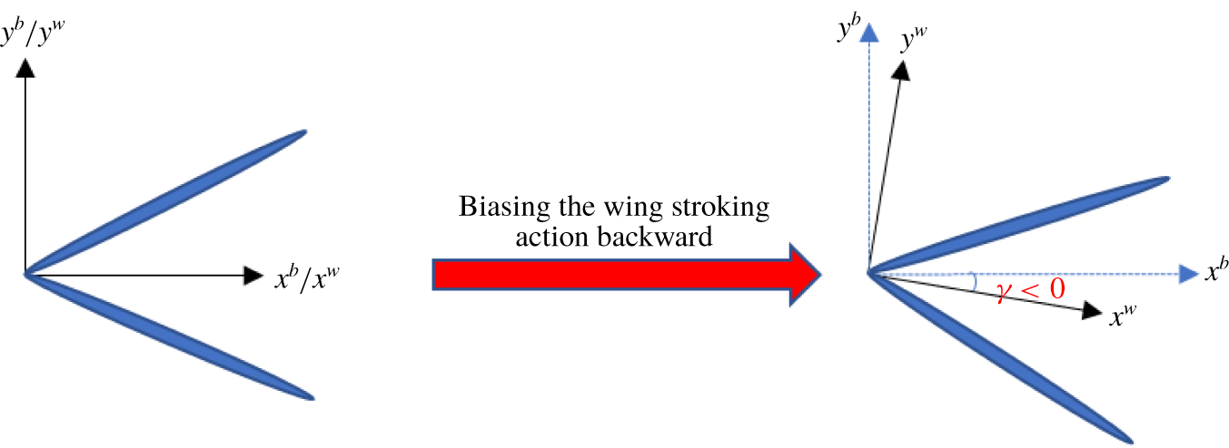
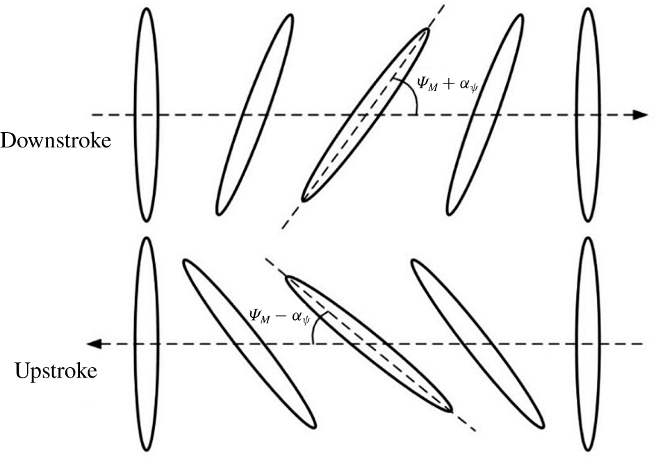
 $(x,y,z)^{n}$ and its motion is described by the rotation of the frame relative to the wing frame
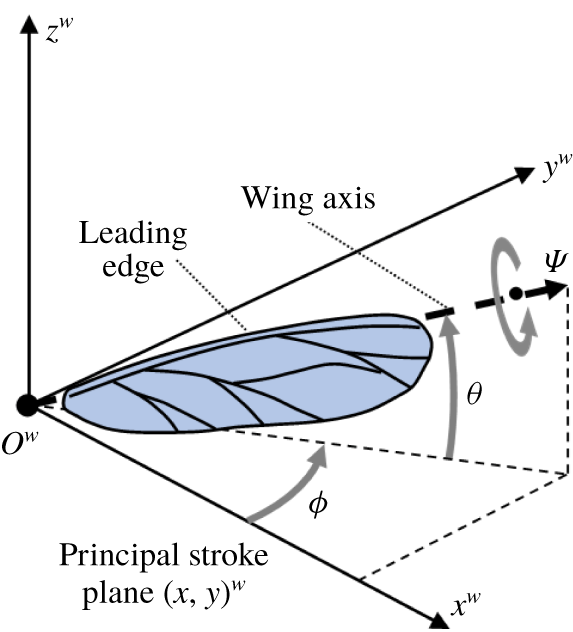
 $(x,y,z)^{w}$ in figure 2, where the
 $(x,y)^{w}$-plane denotes the principal stroke (sweep) plane. The rotation is specified by the three wing angles: the stroke/sweep angle (
 $\unicode[STIX]{x1D719}$) about the
 $z^{w}$-axis, the elevation angle (
 $\unicode[STIX]{x1D703}$) about the principal stroke plane, and the twist angle (
 $\unicode[STIX]{x1D713}$) about the wing axis (dashed arrow). The wing angles
 $\unicode[STIX]{x1D719}$,
 $\unicode[STIX]{x1D703}$ and
 $\unicode[STIX]{x1D713}$ are essentially the Euler angles. They specify the action of the wings during flight, and are thus prescribed or actively controlled functions of time
 $t$. The wing frame
 $(x,y,z)^{w}$ is in turn affixed to the model insect at the wing roots, and aligned with the body frame
 $(x,y,z)^{b}$ at time
 $t=0$.
Schematic diagram of the wing angles ( $\unicode[STIX]{x1D719},\unicode[STIX]{x1D703},\unicode[STIX]{x1D713}$) in the wing frame
 $(x,y,z)^{w}$.

Wing kinematics directly affects the production of aerodynamic forces and moments during insect flight. The wing kinematics of various insects have been described by many researchers (Ellington Reference Ellington1984b; Willmott & Ellington Reference Willmott and Ellington1997a; Altshuler et al. Reference Altshuler, Dickson, Vance, Roberts and Dickinson2005; Fry, Sayaman & Dickinson Reference Fry, Sayaman and Dickinson2005), who showed that insects could employ fairly complex wing kinematics during flight. Complex kinematics could be decomposed into a Fourier series of sinusoidal functions. However, the leading-order harmonics generally dominate the production of forces and moments, and the contributions of the higher harmonics are not well understood due to the nonlinear nature of the aerodynamics. From a flight control viewpoint, low-order kinematic approximations that employ a small set of control parameters are much to be preferred. Low-order Fourier series comprising simple sinusoidal functions are probably also the most natural and optimal for describing the periodic or quasi-periodic wing kinematics of the present model flyer. For the present study, the wing angle functions may be represented as follows:
 $$\begin{eqnarray}\displaystyle & \displaystyle \unicode[STIX]{x1D719}(t)=-{\displaystyle \frac{(\unicode[STIX]{x1D6F7}\pm \unicode[STIX]{x1D6FF}_{SA})}{2}}\cos (2\unicode[STIX]{x03C0}t), & \displaystyle\end{eqnarray}$$
 $$\begin{eqnarray}\displaystyle & \displaystyle \unicode[STIX]{x1D703}(t)=\unicode[STIX]{x1D703}_{a}\sin (2\unicode[STIX]{x03C0}t), & \displaystyle\end{eqnarray}$$
 $$\begin{eqnarray}\displaystyle & \displaystyle \unicode[STIX]{x1D713}(t)={\displaystyle \frac{\unicode[STIX]{x03C0}}{2}}-\left({\displaystyle \frac{\unicode[STIX]{x03C0}}{4}}\pm \unicode[STIX]{x1D6FC}_{\unicode[STIX]{x1D713}}\right)\sin (2\unicode[STIX]{x03C0}t), & \displaystyle\end{eqnarray}$$
 $t$ is the non-dimensional time. Here
 $\pm \unicode[STIX]{x1D6FF}_{SA}$ denotes the difference in the stroke amplitude of the left and right wings, while
 $\pm \unicode[STIX]{x1D6FC}_{\unicode[STIX]{x1D713}}$ is the difference in the angle of attack (AoA) of the two wings at their mid-stroke. The
 $\unicode[STIX]{x1D703}_{a}$ defines the wing elevation amplitude for an oval-shaped wing motion, which is an important control action for forward flight.
3 Computational model
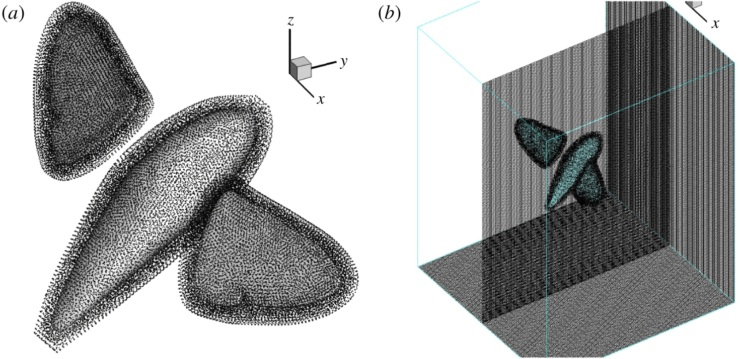
The numerical model comprises the 3-D incompressible viscous fluid flow equations and the Newtonian equations of the model flyer, which were solved in a dynamically coupled manner (see appendix B). A mesh/time-step size independence study was first carried out to determine the appropriate domain size, grid density and time resolution that gave a good trade-off between numerical accuracy and cost for the intensive computation that was entailed. The optimal computational domain was determined to be  $10\times 10\times 10$, with a Cartesian mesh interval at 0.025 wing length. The model insect was wrapped within a cloud of 59 959 mesh-free nodes that give a finer resolution than the background mesh. A final non-dimensional time step of 0.002 was selected. The accuracy of computational model was verified against published results for falling spheres (Mordant & Pinton Reference Mordant and Pinton2000) and flapping wings (Lua et al. Reference Lua, Lee, Lim and Yeo2016) at Reynolds numbers relevant to the present work. In addition, the hawkmoth model was simulated under the condition of zero external forcing to verify that the dynamics of flapping-wing mass was correctly implemented in the flyer model, and the results were further checked against analytical results from an equivalent simplified Newtonian representation of the flyer. Interested readers may refer to Yao (Reference Yao2018) and Yao & Yeo (Reference Yao and Yeo2019a) for further details.
4 Wing kinematics adjustment and flight control
4.1 Control algorithm
The control for free hovering flight has been explained and tested by Wu et al. (Reference Wu, Yeo and Lim2014) in the case of the small fruit fly D. melanogaster. Yao & Yeo (Reference Yao and Yeo2019b) further analysed the control stability of insect hovering flight based on the same control mechanisms by developing a simplified dynamic model of the flyer and flow. The basic flight control strategies used in the present study of forward flight are an extension of what they had done. A generic proportional–integral–derivative (PID)-based feedback control algorithm is used here, which comprises three components: a proportional component that reflects the current deviation/error  $\boldsymbol{e}(t)=(\boldsymbol{X}_{B},\unicode[STIX]{x1D723})(t)-(\boldsymbol{X}_{B},\unicode[STIX]{x1D723})_{D}$ of the current configuration (or flight state) of the flyer from the desired configuration
 $(\boldsymbol{X}_{B},\unicode[STIX]{x1D723})_{D}$; an integral component that considers the accumulated error
 $\int \boldsymbol{e}(\unicode[STIX]{x1D70F})\,\text{d}\unicode[STIX]{x1D70F}$; and a differential component
 $\text{d}\boldsymbol{e}/\text{d}t$ for estimating future error. The vector
 $(\boldsymbol{X}_{B},\unicode[STIX]{x1D723})(t)$ describes the displacement
 $\boldsymbol{X}_{B}$ and orientation
 $\unicode[STIX]{x1D723}$ of the flyer. The kinematic control vector
 $\boldsymbol{U}(t)$ is computed as a weighted sum of the three components:
 $$\begin{eqnarray}\boldsymbol{U}(t)=\boldsymbol{k}_{p}\boldsymbol{e}(t)+\boldsymbol{k}_{d}{\displaystyle \frac{\text{d}}{\text{d}t}}\boldsymbol{e}(t)+\boldsymbol{k}_{i}\int _{0}^{t}\boldsymbol{e}(\unicode[STIX]{x1D70F})\,\text{d}\unicode[STIX]{x1D70F}+\boldsymbol{U}_{0},\end{eqnarray}$$
where  $\boldsymbol{k}_{p}$,
 $\boldsymbol{k}_{i}$ and
 $\boldsymbol{k}_{d}$ are the control coefficient matrices – these need to be specified to fully define the controller. The vector
 $\boldsymbol{U}(t)$ comprises updated kinematic control parameters to be used over the ensuing control cycle, where
 $\boldsymbol{U}_{0}$ denotes the initial or baseline state. The control parameters involved in the current study are introduced in the sections that follow and the appendices; readers may refer to Wu et al. (Reference Wu, Yeo and Lim2014), Yao (Reference Yao2018) and Yao & Yeo (Reference Yao and Yeo2019b) for further information. Initial estimates of the control coefficients were first obtained from the simplified dynamic model (Yao & Yeo Reference Yao and Yeo2019b) for hovering flight, which were then refined via full CFD–FSI (fluid–structure interaction) simulations before final adoption. At the start of a new wing cycle, the PID controller first calculates
 $\boldsymbol{U}(t)$ according to the current error state
 $\boldsymbol{e}(t)$. Then
 $\boldsymbol{U}(t)$ is linearly applied to smoothly correct the wing motion over the ensuing cycle to reduce the deviation. Bounds were set on
 $\boldsymbol{U}(t)$ to prevent geometric conflict (wing–body collision) and to avoid overflowing control response during simulation.
Potential delay/latency between feedback and control action was not considered in this study, due in part to a lack of definitive data concerning the stimuli–neural–motor response of the insect, and a desire to minimize the number of free variables in the problem. Analysis based on the simplified dynamics model of Yao & Yeo (Reference Yao and Yeo2019b) shows that latency would cause a softening of the longitudinal PID control coefficients, by the order of 10 %–20 % and 20 %–40 % for half- and one-cycle control latency, respectively, depending on the individual coefficient, which were also verified by model simulations. Similar ranges of control coefficients are also applicable to cases where the interval of control intervention is extended to two and three wing cycles, respectively, instead of the one cycle used in this study.
4.2 Forward flight control
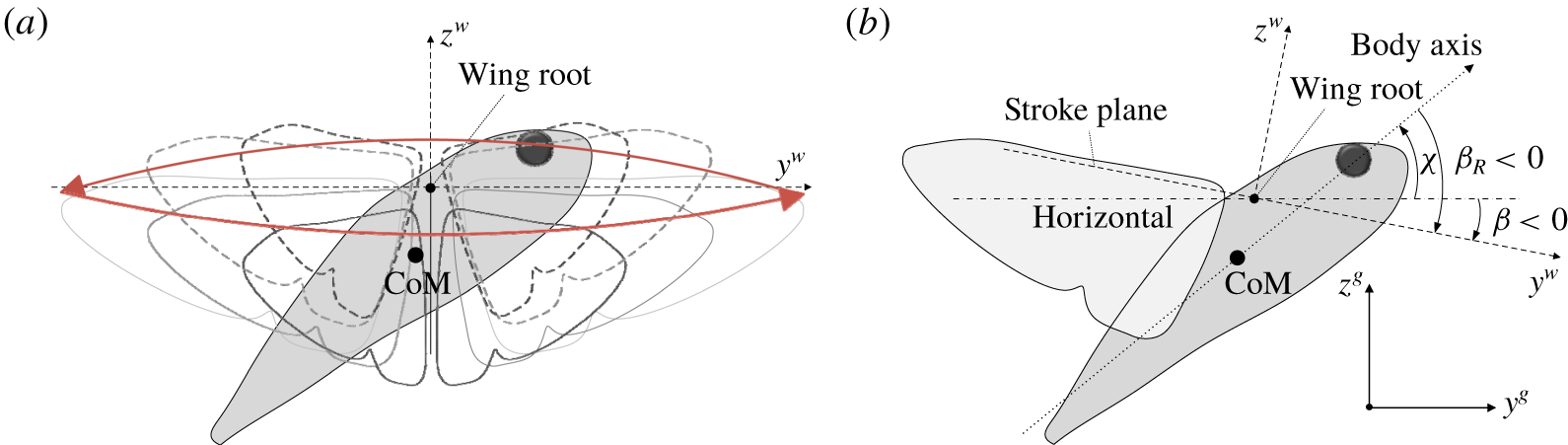
Insects frequently launch themselves into forward rectilinear flight from an initial hovering stage. This involves a pitching down action, which directs a component of the lift force forwards, and accelerating to gain speed. The former may be accomplished within a few wing cycles, and help to reduce the profile drag by better aligning the body of the insect with the direction of travel. The more prolonged second stage requires the insect to maintain stable body pitch and height. Rapid pitch down is facilitated by adopting an anticlockwise oval-shaped elevated wing motion (figure 3a), which produces an excessive of negative aerodynamic- and wing-inertia-induced  $x$-moment over a wing cycle. The net negative aerodynamic moment may be intuitively attributed to the smaller moment arm of the drag acting on the wings about the centre of mass (CoM) as they sweep below the wing roots in the downstroke, compared with the same as the wings sweep above the wing roots in the upstroke. Concurrently, the anticlockwise motion of the wing mass also induces a clockwise (pitch-down) inertia-driven rotation of the body, which is roughly proportional to the wing mass. The aerodynamic and inertia moments could combine to help the insect pitch down rapidly over several wing cycles, when a suitable value of the elevation angle
 $\unicode[STIX]{x1D703}_{a}$ is specified in (2.3b).
Illustrations of wing motion and body orientation in forward flight. (a) Oval-shaped wing motion. (b) Body pitching angle ( $\unicode[STIX]{x1D712}$), stroke-plane pitching angle relative to the body axis (
 $\unicode[STIX]{x1D6FD}_{R}$) and stroke-plane pitching angle made with the global horizontal direction (
 $\unicode[STIX]{x1D6FD}=\unicode[STIX]{x1D712}+\unicode[STIX]{x1D6FD}_{R}$).

After the initial downward pitch to a more horizontal body posture, the insect has to maintain a steady body pitch as it accelerates forwards towards its chosen cruising speed. Earlier study by Yao & Yeo (Reference Yao and Yeo2018) showed that an insect flyer would likely encounter rising pitch-up moment as it gathers forward speed. This is due to higher relative air flow over the wings (higher drag) in the downstrokes vis-à-vis the upstrokes, and the height of the wings above the CoM. A series of simulations were thus carried out first to quantify the aerodynamic forces and moments that the model flyer might encounter over a projected range of non-dimensional speeds ( $1<v/(\,f_{0}L)<3$) and body stroke-plane angles (
 $-75^{\circ }<\unicode[STIX]{x1D6FD}_{R}<-55^{\circ }$). This gives stroke-plane angle
 $-70^{\circ }<\unicode[STIX]{x1D6FD}<-50^{\circ }$ when the body is pitched at the desired body angle of
 $\unicode[STIX]{x1D712}=5^{\circ }$ (see figure 3b). Johansson et al. (Reference Johansson, Engel, Kelber, Heerenbrink and Hedenström2013) showed that a hummingbird hawkmoth’s wingbeat frequency could go up to 82.4 Hz during forward flight, whereas the present model hawkmoth has a reference frequency of
 $f_{0}\approx 65~\text{Hz}$ for equilibrium hovering (Yao & Yeo Reference Yao and Yeo2019a). The prescribed forward motion study was thus carried out at a middling wingbeat frequency of
 $f=75~\text{Hz}$.
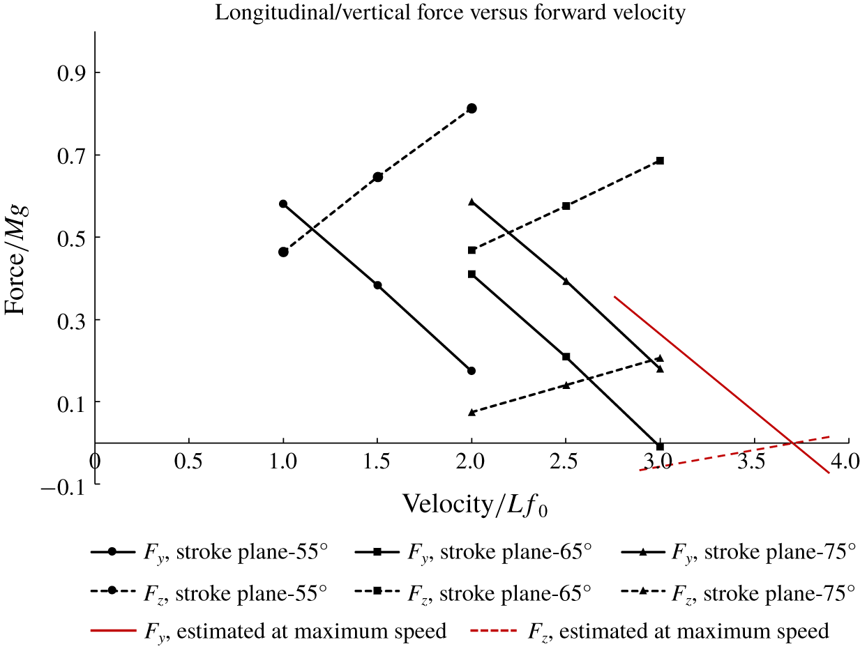
Variations of net cycle-mean aerodynamic forces with forward speed  $v/(\,f_{0}L)$ at different body stroke-plane angles (
 $\unicode[STIX]{x1D6FD}_{R}$) relative to the equilibrium hovering state. Longitudinal force
 $F_{y}$ (solid lines) and vertical force
 $F_{z}$ (dashed lines).

Figure 4 shows that the net longitudinal force ( $F_{y}$) and vertical force (
 $F_{z}$) vary quite linearly with the forward speed over the selected range of body stroke-plane angle
 $\unicode[STIX]{x1D6FD}_{R}$. As
 $\unicode[STIX]{x1D6FD}_{R}$ gets smaller, the curves shift from left to right for both
 $F_{y}$ and
 $F_{z}$. In addition,
 $F_{y}$ and
 $F_{z}$ also vary quite linearly with respect to
 $\unicode[STIX]{x1D6FD}_{R}$ because the curves remain roughly parallel and even in their intervals as
 $\unicode[STIX]{x1D6FD}_{R}$ varies. Furthermore, both
 $F_{y}$ and
 $F_{z}$ could only go negative when
 $\unicode[STIX]{x1D6FD}_{R}$ is beyond
 $-75^{\circ }$; here the speed limitation for
 $f=75~\text{Hz}$ is reached. This is marked by the intersection of the two red lines in figure 4, which represent the force variation with speed at the body stroke-plane angle
 $\unicode[STIX]{x1D6FD}_{R}\approx -80^{\circ }$. The effects of forward speed and body stroke-plane angle
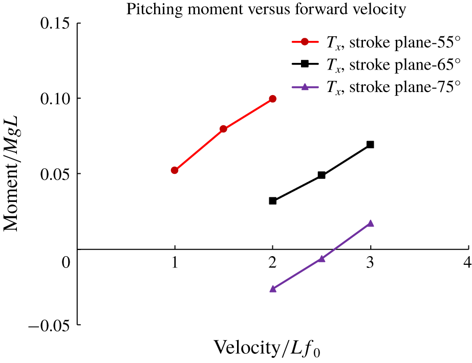
 $\unicode[STIX]{x1D6FD}_{R}$ on the cycle-mean pitching moment (
 $T_{x}$) acting on the flyer are depicted in figure 5. Here we note that
 $T_{x}$ increases at a significant and nearly linear rate with the speed for all values of
 $\unicode[STIX]{x1D6FD}_{R}$.
In free insect hovering flight, stable pitch control can generally be achieved by just varying the mean positional angle ( $\unicode[STIX]{x1D6FE}$) of the unelevated wing strokes, which affects the mean aerodynamic pitching moment produced by the wings over a wing cycle (Wu et al. Reference Wu, Yeo and Lim2014; Yao Reference Yao2018; Yao & Yeo Reference Yao and Yeo2019b). However, this means of generating pitching moment to control and stabilize the posture of the insect may not be sufficient for an insect in forward flight at a significant speed due to the large buildup in pitch-up moment as indicated in figure 5. Pitch control for an insect in fast forward flight clearly requires an additional mechanism for generating a countering pitch-down torque. This had to some extent been anticipated by our earlier discussion concerning the role of wing elevation to pitch down the flyer in the first stage of forward flight. The combined action of wing elevation angle (
 $\unicode[STIX]{x1D703}_{a}$) and mean positional angle (
 $\unicode[STIX]{x1D6FE}$) to counter the persistent pitching-up tendency of the flyer during forward flight, and to stabilize its pitch angle at the desired value, has been discussed by Yao & Yeo (Reference Yao and Yeo2018) in the context of a small fruit fly model. The same strategy is used here with some modifications.
In keeping with the linear increase in the cycle-mean pitch-up moment ( $T_{x}$) with the forward speed (
 $v$), the elevation angle (
 $\unicode[STIX]{x1D703}_{a}$) of the wings may be set in accordance with a simple linear relation of the form
 $$\begin{eqnarray}\unicode[STIX]{x1D703}_{a}=k^{\unicode[STIX]{x1D703}}v.\end{eqnarray}$$
Figure 5 shows that  $k^{\unicode[STIX]{x1D703}}$ is not a constant, but is dependent on the body stroke-plane angle (
 $\unicode[STIX]{x1D6FD}_{R}$) of the wings. However, the latter is also involved in conjunction with other kinematic parameters to control the speed and height of flight by the PID controller. In this work,
 $k^{\unicode[STIX]{x1D703}}$ is increased or decreased alternately to counter any detected tendency of the model hawkmoth to pitch up or down, respectively, and not directly tied to the value of
 $\unicode[STIX]{x1D6FD}_{R}$.
Variations of cycle-mean pitching moment with forward speed  $v$ at different body stroke-plane angles
 $\unicode[STIX]{x1D6FD}_{R}$, with set
 $\unicode[STIX]{x1D712}=5^{\circ }$.

Overall, the cycle-mean dynamics of controlled longitudinal flight may be shown to be governed by a state-variable equation of motion of the form,
 $$\begin{eqnarray}\dot{\boldsymbol{x}}=\unicode[STIX]{x1D63C}\,\boldsymbol{x}+\unicode[STIX]{x1D743},\end{eqnarray}$$
with
 $$\begin{eqnarray}\boldsymbol{x}=\left(\begin{array}{@{}c@{}}v\\ w\\ \dot{\unicode[STIX]{x1D712}}\end{array}\right),\quad \unicode[STIX]{x1D63C}=\left[\begin{array}{@{}ccc@{}}{\displaystyle \frac{1}{M}}Y_{v} & {\displaystyle \frac{1}{M}}Y_{w} & {\displaystyle \frac{1}{M}}Y_{\dot{\unicode[STIX]{x1D712}}}\\ {\displaystyle \frac{1}{M}}Z_{v} & {\displaystyle \frac{1}{M}}Z_{w} & {\displaystyle \frac{1}{M}}Z_{\dot{\unicode[STIX]{x1D712}}}\\ {\displaystyle \frac{1}{I_{xx}}}P_{v} & {\displaystyle \frac{1}{I_{xx}}}P_{w} & {\displaystyle \frac{1}{I_{xx}}}P_{\dot{\unicode[STIX]{x1D712}}}\end{array}\right],\quad \unicode[STIX]{x1D743}=\left(\begin{array}{@{}c@{}}{\displaystyle \frac{F_{f}}{M}}\sin (-\unicode[STIX]{x1D6FD})\\ {\displaystyle \frac{F_{f}}{M}}\cos (-\unicode[STIX]{x1D6FD})\\ {\displaystyle \frac{P_{\unicode[STIX]{x1D6FE}}}{I_{xx}}}\unicode[STIX]{x1D6FE}+{\displaystyle \frac{P_{\unicode[STIX]{x1D703}}}{I_{xx}}}\unicode[STIX]{x1D703}_{a}\end{array}\right),\end{eqnarray}$$
which shows how the above-mentioned kinematic actions come together to foster longitudinal flight. Here  $\boldsymbol{x}$ denotes the longitudinal flight vector comprising the horizontal (
 $v$) and vertical (
 $w$) translational and the angular pitching (
 $\dot{\unicode[STIX]{x1D712}}$) velocity deviations of the flyer from its reference flight state. The matrix
 $\unicode[STIX]{x1D63C}$ consists of stability derivatives, which govern the ‘natural’ coupled body–fluid response of the flyer to forces/moments arising from the velocity deviations
 $\boldsymbol{x}$ of the flyer, while the vector
 $\unicode[STIX]{x1D743}$ represents forces/moments due solely to the kinematic actions of the wings. Here
 $F_{f}$ denotes the magnitude of wing force in the (
 $y,z$)-plane; while
 $P_{\unicode[STIX]{x1D6FE}}$ and
 $P_{\unicode[STIX]{x1D703}}$ are coefficients governing the pitching moment generated by the control angles
 $\unicode[STIX]{x1D6FE}$ (mean positional angle) and
 $\unicode[STIX]{x1D703}_{a}$ (wing elevation angle), respectively, and
 $I_{xx}$ is the moment of inertia about the CoM axis
 $x^{b}$ (figure 1a).
The lateral dynamics is ignored in this representation for simplicity, as their effects are of a higher order. Comparison of state equation (4.3) with a typical second-order dynamical system (say a spring–mass system) shows that the matrix ( $-\unicode[STIX]{x1D63C}$) comprises coefficients of motion damping. The absence of an intrinsic restoring mechanism (spring-like terms) indicates that the natural fluid–body system as represented by
 $\dot{\boldsymbol{x}}=\unicode[STIX]{x1D63C}\,\boldsymbol{x}$ is essentially unstable – and stable longitudinal flight is only possible with ‘artificial’ intervention by kinematic control action via the vector
 $\unicode[STIX]{x1D743}$, which performs dual roles of maintaining stable flight as well as directing the flight. The coefficients in (4.3) could be estimated theoretically from the prescribed motion simulations in the CFD model.
Only the stability derivatives related to the longitudinal velocity  $v$ are important to forward flight dynamics, and the above equation can be simplified to
 $$\begin{eqnarray}\left(\begin{array}{@{}c@{}}\dot{v}\\ {\dot{w}}\\ \ddot{\unicode[STIX]{x1D712}}\end{array}\right)=\left(\begin{array}{@{}c@{}}{\displaystyle \frac{vY_{v}}{M}}-{\displaystyle \frac{F_{f}}{M}}\sin (\unicode[STIX]{x1D6FD}_{R}+\unicode[STIX]{x1D712})\\ {\displaystyle \frac{vZ_{v}}{M}}-{\displaystyle \frac{F_{f}}{M}}\cos (\unicode[STIX]{x1D6FD}_{R}+\unicode[STIX]{x1D712})\\ {\displaystyle \frac{v}{I_{xx}}}\text{}\underline{(P_{v}+P_{\unicode[STIX]{x1D703}}k^{\unicode[STIX]{x1D703}})}_{=0}+{\displaystyle \frac{P_{\unicode[STIX]{x1D6FE}}}{I_{xx}}}\unicode[STIX]{x1D6FE}\end{array}\right).\end{eqnarray}$$
We note that  $\unicode[STIX]{x1D6FD}_{R}$ and
 $\unicode[STIX]{x1D6FE}$ are control angles that are governed by the PID controller, as is also the frequency
 $f$, which affects the magnitude of wing force
 $F_{f}$. Equation (4.4) encapsulates the central dynamics of controlled longitudinal flight that allows us to see how the angles are involved in the control of flight. Incorporating the PID equation (4.1) into
 $\unicode[STIX]{x1D743}$ indirectly introduces recovery or stiffness (proportional) terms that act against motion deviation, and modifies motion damping in the full state equation. For pitch control, it is desirable to minimize the
 $(P_{v}+P_{\unicode[STIX]{x1D703}}k^{\unicode[STIX]{x1D703}})$ term in (4.4) – this amounts to applying the appropriate wing elevation to counter the pitch-up moment induced by its longitudinal speed
 $v$. This frees up the PID mechanism to stabilize the body pitch angle
 $\unicode[STIX]{x1D712}$ near its designated value via the mean-positional angle
 $\unicode[STIX]{x1D6FE}$.
During the acceleration stage, the wingbeat frequency is set to a fixed value of  $f=75~\text{Hz}$ for the current study. The stroke-plane pitching angle (
 $\unicode[STIX]{x1D6FD}_{R}$) is then adjusted by the PID controller to maximize the forward force, with just sufficient vertical force to support the insect weight and maintain the height of the insect. As the insect gains speed, it will eventually come up against its upper limit set by the wingbeat frequency; marked by the intersection of the two red lines in figure 4. A hummingbird hawkmoth may cruise at a lower speed for better energy efficiency, by switching from acceleration to cruising mode as it approaches the desired speed. The mechanism for pitch control remains the same for constant-speed cruising as for accelerating flight, while the PID algorithm constantly adjusts the wingbeat frequency (
 $f$) and body stroke-plane angle (
 $\unicode[STIX]{x1D6FD}_{R}$) in tandem to simultaneously maintain the height and forward speed
 $v$ of the flyer. In these regards,
 $f$ now determines the total wing force generated by the flapping motion, whose vertical component supports the weight of the flyer, while
 $\unicode[STIX]{x1D6FD}_{R}$ regulates the longitudinal wing force to balance the drag.
The state-equation model consolidates the central two-dimensional longitudinal dynamics of controlled forward flight into an accessible form, in which the roles of the kinematic control actions are clearly identified. The reduced form (4.4) can be helpful for establishing control coefficients for stable flight, as in Yao & Yeo (Reference Yao and Yeo2019b), when combined with a suitable wing force model. The actual ‘real-time’ simulations of controlled longitudinal free flight are, however, carried in full 3-D space in accordance with the methodologies of §§ 4.1 and 3.
4.3 Sideslip manoeuvre control
Sideslipping is an important skill for a hawkmoth, where it effectively translates itself in a parallel fashion laterally to a new position. With it, a hawkmoth could easily reposition itself during foraging and dodge predator attack rapidly. This is unlike the case for most birds, where sideways flight is accomplished by a banking turn and flying forward in the new direction. A generic sideslip manoeuvre typically commences with the flyer in a hovering state. In the present study, the model hawkmoth is required to translate laterally to its right and to resume hovering at a new prescribed position some distance away. Unlike forward flight, where the insect only accelerates to the required cruising speed, here it goes through an acceleration–deceleration process during the sideslip manoeuvre.
The most significant motion during a sideslip manoeuvre is body rolling and lateral translation – rolling directs a component of the hovering lift force to initiate and drive the translation. As for forward flight, prescribed motion simulations were first conducted to determine the aerodynamic forces ( $F_{x}$ and
 $F_{z}$) and the roll and yaw moments (
 $T_{y}$ and
 $T_{z}$) induced by sideslip translation, with focus on the effects of sideslip/lateral velocity (
 $u$), body rolling velocity (
 $\dot{\unicode[STIX]{x1D702}}$) and body roll angle (
 $\unicode[STIX]{x1D702}$). The wingbeat frequency was set at
 $f=f_{0}=65~\text{Hz}$, which generates a cycle-mean lift roughly equal to the weight of the insect in hovering. The results are summarized in figures 6–8, where the forces and moments are given with respect to the body frame
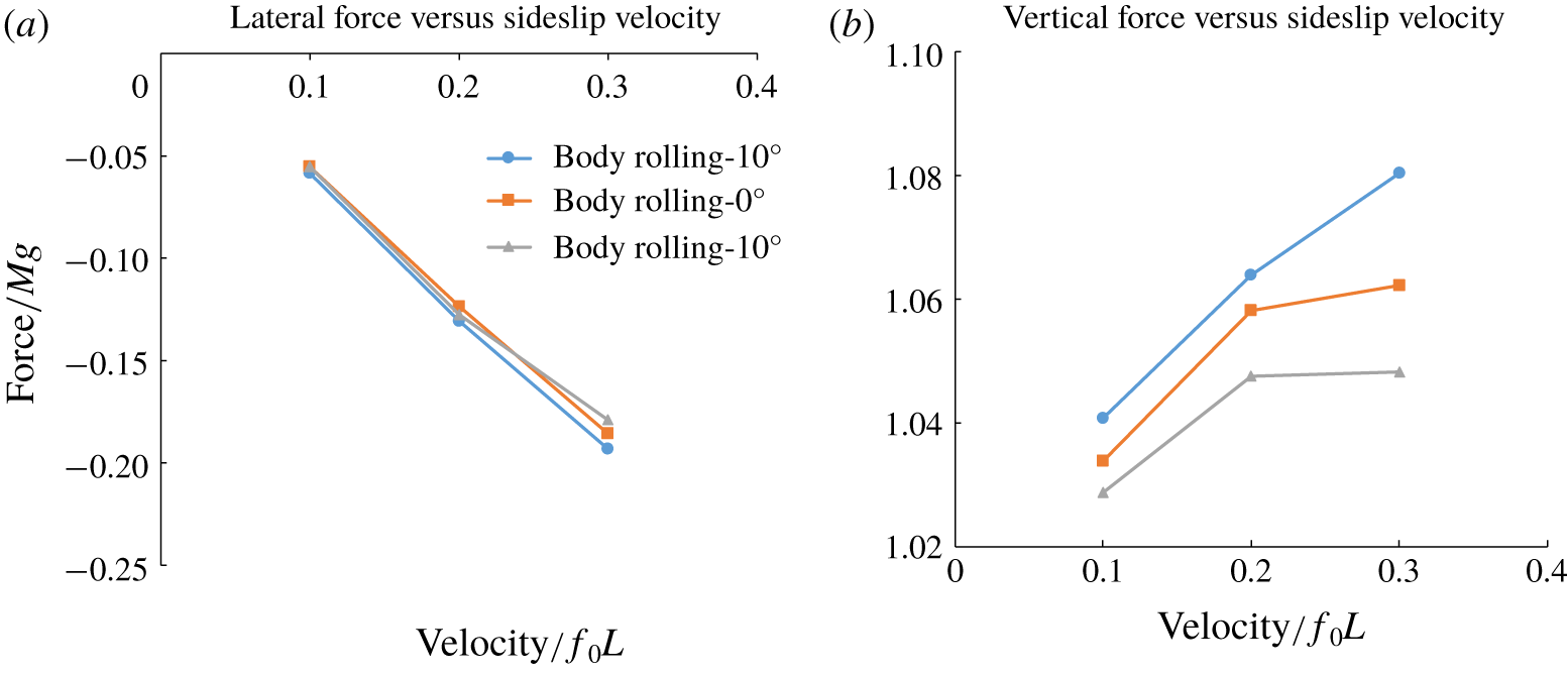
 $(x,y,z)^{b}$ of the flyer. Figure 6(a) shows that the aerodynamic resistance (
 $-F_{x}$) to lateral translation rises with its velocity
 $u$, and its variations are largely indifferent to the rolled posture of the insect for
 $-10^{\circ }\leqslant \unicode[STIX]{x1D702}\leqslant 10^{\circ }$. The lift force (figure 6b) is, on the other hand, consistently enhanced by the translation-induced lateral airflow. The boost may be explained by the asymmetry of the wing strokes to the oncoming side flow – where those parts of the strokes of the two wings that experience increased relative airflow produce increased lift, which more than compensates for drops in lift over the other parts that encounter reduced relative airflow. Negative roll (
 $\unicode[STIX]{x1D702}=-10^{\circ }$), which exposes the under-face of the wings to the side flow
 $u$, enjoys greater lift enhancement. For roll-induced translation (
 $\unicode[STIX]{x1D702}=10^{\circ }$) the lift increase levels off at approximately 4 % for
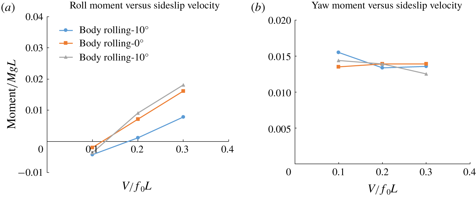
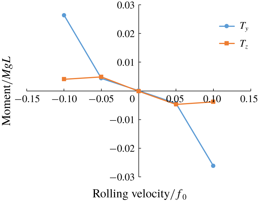
 $0.2<u/(\,f_{0}L)<0.3$. Positive rolling and yawing moments are induced by the positive lateral speed; rolling moment varies roughly linearly while the yaw moment remains almost the same for all lateral speeds (figure 7). Moment variations with rolling velocity (figure 8) are less linear compared with the force variations with respect to sideslip velocity (figure 6).
Force variations with sideslip speed.

Moment variations with sideslip speed.

Moment variations with rolling speed.

The leading dynamics of sideslip manoeuvre for the hawkmoth is again highly two-dimensional, and the cycle-mean lateral motion may also be represented in state-variable form as given by (4.5) below. Owing to the presence of large variation of body angles in sideslip manoeuvre, the state equations are defined here with respect to the body frame:
 $$\begin{eqnarray}\dot{\boldsymbol{x}}=\unicode[STIX]{x1D63D}(\unicode[STIX]{x1D63C}\,\boldsymbol{x}+\unicode[STIX]{x1D743}),\end{eqnarray}$$
with
 $$\begin{eqnarray}\displaystyle & \displaystyle \boldsymbol{x}=\left(\begin{array}{@{}c@{}}u\\ \dot{\unicode[STIX]{x1D702}}\\ \dot{\unicode[STIX]{x1D701}}\end{array}\right),\quad \unicode[STIX]{x1D63C}=\left[\begin{array}{@{}ccc@{}}X_{u}\cos \unicode[STIX]{x1D702}+Z_{u}\sin \unicode[STIX]{x1D702} & X_{\dot{\unicode[STIX]{x1D702}}} & X_{\dot{\unicode[STIX]{x1D701}}}\\ R_{u} & R_{\dot{\unicode[STIX]{x1D702}}} & R_{\dot{\unicode[STIX]{x1D701}}}\\ Q_{u} & Q_{\dot{\unicode[STIX]{x1D702}}} & Q_{\dot{\unicode[STIX]{x1D701}}}\end{array}\right],\quad \unicode[STIX]{x1D743}=\left(\begin{array}{@{}c@{}}Mg\tan (\unicode[STIX]{x1D702}+\unicode[STIX]{x1D703}_{R})\\ R_{\unicode[STIX]{x1D6FF}}\unicode[STIX]{x1D6FF}_{SA}\\ Q_{\unicode[STIX]{x1D6FC}}\unicode[STIX]{x1D6FC}_{\unicode[STIX]{x1D713}}\end{array}\right), & \displaystyle \nonumber\\ \displaystyle & \displaystyle \unicode[STIX]{x1D63D}=\left[\begin{array}{@{}ccc@{}}{\displaystyle \frac{1}{M}} & 0 & 0\\ 0 & {\displaystyle \frac{I_{zz}}{I_{yy}I_{zz}-I_{yz}^{2}}} & {\displaystyle \frac{I_{yz}}{I_{yy}I_{zz}-I_{yz}^{2}}}\\ 0 & {\displaystyle \frac{I_{yz}}{I_{yy}I_{zz}-I_{yz}^{2}}} & {\displaystyle \frac{I_{yy}}{I_{yy}I_{zz}-I_{yz}^{2}}}\end{array}\right], & \displaystyle \nonumber\end{eqnarray}$$
where  $\unicode[STIX]{x1D63D}$ is the inertia matrix. Matrix
 $\unicode[STIX]{x1D63C}$ contains the stability derivatives for sideslip motion, which have similar meaning to those for forward flight. The control vector
 $\unicode[STIX]{x1D743}$ is again associated with the force/moment generated by kinematic control actions. The components of
 $\unicode[STIX]{x1D743}$ correspond, respectively, to: (i) the lateral force in the global frame which is governed by the roll angle of the body (
 $\unicode[STIX]{x1D702}$) and roll angle of the stroke plane about the body (
 $\unicode[STIX]{x1D703}_{R}$); (ii) the roll torque generated by stroke amplitude difference (
 $\unicode[STIX]{x1D6FF}_{SA}$) of the two wings; and (iii) the yaw torque arising from mid-stroke AoA difference (
 $\unicode[STIX]{x1D6FC}_{\unicode[STIX]{x1D713}}$) between the two wings. Coefficients
 $R_{\unicode[STIX]{x1D6FF}}$ and
 $Q_{\unicode[STIX]{x1D6FC}}$ are related to the kinematics and geometry of the flyer. These and the components of matrix
 $\unicode[STIX]{x1D63C}$ could theoretically be determined from prescribed motion CFD simulations. The
 $I_{yy}$ and
 $I_{zz}$ are the moments of inertia of the body about the
 $y^{b}$- and
 $z^{b}$-axes as shown in figure 1(a), while
 $I_{yz}$ is the cross-moment of inertia that couples roll–yaw motion.
The values of the stability derivatives in matrix  $\unicode[STIX]{x1D63C}$ (
 $X_{u},Z_{u},R_{\dot{\unicode[STIX]{x1D702}}},Q_{\dot{\unicode[STIX]{x1D702}}},\ldots$) can be approximated by the gradients in figures 6–8. Since the most prominent motion involved in sideslip is lateral translation and rolling, only derivatives related to the lateral velocity
 $u$ and the rate of rolling
 $\dot{\unicode[STIX]{x1D702}}$ are of significance here. Furthermore, derivatives relating to the effect of rolling angle in figures 6(a) and 7(a) can also be ignored, since they would not bring about notable changes in the force or moment. Equation (4.5) can thus be simplified to
 $$\begin{eqnarray}\left(\begin{array}{@{}c@{}}\dot{u}\\ \ddot{\unicode[STIX]{x1D702}}\\ \ddot{\unicode[STIX]{x1D701}}\end{array}\right)=\unicode[STIX]{x1D63D}\left(\begin{array}{@{}c@{}}uX_{u}\cos \unicode[STIX]{x1D702}+uZ_{u}\sin \unicode[STIX]{x1D702}+Mg\tan (\unicode[STIX]{x1D702}+\unicode[STIX]{x1D703}_{R})\\ uR_{u}+\dot{\unicode[STIX]{x1D702}}R_{\dot{\unicode[STIX]{x1D702}}}+R_{\unicode[STIX]{x1D6FF}}\unicode[STIX]{x1D6FF}_{SA}\\ uQ_{u}+\dot{\unicode[STIX]{x1D702}}Q_{\dot{\unicode[STIX]{x1D702}}}+Q_{\unicode[STIX]{x1D6FC}}\unicode[STIX]{x1D6FC}_{\unicode[STIX]{x1D713}}\end{array}\right).\end{eqnarray}$$
Greeter & Hedrick (Reference Greeter and Hedrick2016) have shown that a hawkmoth performs sideslip manoeuvre by rolling its body and wings to reorient the lift force in the global frame. To execute a sideslip, a flyer first needs to roll its body/wing in the desired direction by differentially changing the stroke amplitudes ( $\unicode[STIX]{x1D6FF}_{SA}$) of the left and right wings; the desired amount of body roll (
 $\unicode[STIX]{x1D702}$) may depend on the expected distance to the targeted position. Upon approaching the target position, negative feedbacks that take into account the lateral speed and distance to target are applied to reverse the rolling of the flyer so as to decelerate it, and re-establish hovering at the target position. Meanwhile, the yaw (
 $\unicode[STIX]{x1D701}$) of the flyer is checked by adjusting the mid-stroke AoA difference
 $\unicode[STIX]{x1D6FC}_{\unicode[STIX]{x1D713}}$, and the height maintained by small changes to the wingbeat frequency
 $f$.
To reduce controller complexity, stroke-plane rolling angle ( $\unicode[STIX]{x1D703}_{R}$) is not utilized to generate a lateral force during the sideslip manoeuvre, but is activated only when the flyer resumes hovering at the new location. Equation (4.6) may be further developed and simplified by choosing the appropriate functional forms for control angles
 $\unicode[STIX]{x1D6FF}_{SA}$ and
 $\unicode[STIX]{x1D6FC}_{\unicode[STIX]{x1D713}}$:
 $$\begin{eqnarray}\displaystyle & \displaystyle \unicode[STIX]{x1D6FF}_{SA}=\left[-{\displaystyle \frac{uR_{u}+\dot{\unicode[STIX]{x1D702}}R_{\dot{\unicode[STIX]{x1D702}}}}{R_{\unicode[STIX]{x1D6FF}}}}\right]+[k^{x}(x_{t}-x)-k^{u}u], & \displaystyle\end{eqnarray}$$
 $$\begin{eqnarray}\displaystyle & \displaystyle \unicode[STIX]{x1D6FC}_{\unicode[STIX]{x1D713}}=\left[-{\displaystyle \frac{uQ_{u}+\dot{\unicode[STIX]{x1D702}}Q_{\dot{\unicode[STIX]{x1D702}}}}{Q_{\unicode[STIX]{x1D6FC}}}}\right]+\left[-{\displaystyle \frac{I_{yz}R_{\unicode[STIX]{x1D6FF}}}{I_{yy}Q_{\unicode[STIX]{x1D6FC}}}}(k^{x}(x_{t}-x)-k^{u}u)\right]. & \displaystyle\end{eqnarray}$$
 $x_{t}$ denotes the targeted position for the sideslipping flyer. With (4.7), the leading lateral dynamics of the sideslipping model hawkmoth is transformed to
 $$\begin{eqnarray}\left(\begin{array}{@{}c@{}}\dot{u}\\ \ddot{\unicode[STIX]{x1D702}}\\ \ddot{\unicode[STIX]{x1D701}}\end{array}\right)=\left(\begin{array}{@{}c@{}}{\displaystyle \frac{uX_{u}\cos \unicode[STIX]{x1D702}+uZ_{u}\sin \unicode[STIX]{x1D702}}{M}}+g\tan \unicode[STIX]{x1D702}\\ \left({\displaystyle \frac{I_{zz}}{I_{yy}I_{zz}-I_{yz}^{2}}}-{\displaystyle \frac{I_{yz}^{2}}{I_{yy}^{2}I_{zz}-I_{yy}I_{yz}^{2}}}\right)R_{\unicode[STIX]{x1D6FF}}(k^{x}(x_{t}-x)-k^{u}u)\\ 0\end{array}\right),\end{eqnarray}$$
where unwanted yawing of the flyer is automatically suppressed by the chosen configuration of the PID controller in (4.7). The reduced state equation (4.8) may permit further analysis to aid the selection of the control coefficients, when the key stability derivatives are determined from prescribed motion CFD simulations. In addition to the control for sideways and body rolling motion, the control for other degrees of motion remains the same as that for hovering flight (see Yao (Reference Yao2018) and Yao & Yeo (Reference Yao and Yeo2019b) for details). As the insect approaches close to the target location, say 0.2 wing lengths, the sideslip manoeuvre controller is deactivated, and full hovering control is activated to stabilize the flyer at the new location. The above briefly explains how the kinematic control protocol is motivated by an analysis of the simplified dynamics of sideslipping flight.
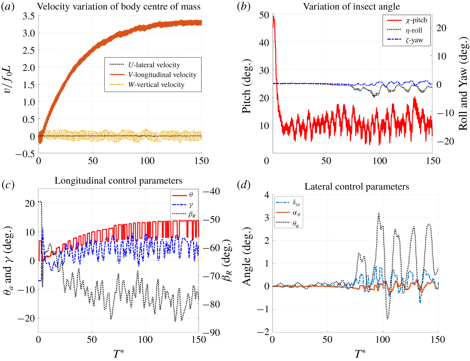
Variation of insect velocity (a), body angles (b) and control parameters (c,d) during forward acceleration flight at  $f=75~\text{Hz}$. Here
 $T^{\ast }$ is the non-dimensional time, obtained by normalizing the dimensional time
 $t$ with the wingbeat frequency
 $f$,
 $T^{\ast }=tf$, so the horizontal axis represents the actual number of wing cycles. Other quantities involved in the current paper, such as the velocity, force and moment, are normalized with reference wingbeat frequency
 $f_{0}=65~\text{Hz}$.

5 Results and discussion
5.1 Forward flight
Forward flights were initiated from the equilibrium hovering status by an increase in the elevation of the wings ( $\unicode[STIX]{x1D703}_{a}=7^{\circ }$) that produces both aerodynamic and inertia torques – this lasted for two to three wing cycles. Simultaneously, the wingbeat frequency
 $f$ was raised from its free hovering value of 65 Hz to 75 Hz to strongly accelerate the flyer forwards. Readers may refer to the supplementary movies for the animation of forward flight available at https://doi.org/10.1017/jfm.2020.361.
5.1.1 Flight performance
The simulation was first carried out for 150 wing cycles (2 s in physical time) to allow the model hawkmoth to reach its maximum speed (figure 9). The insect accelerates very fast over the first 30 wing cycles (0.4 s) to reach a velocity of  $2.0f_{0}L$ (
 $2.63~\text{m}~\text{s}^{-1}$). The model hawkmoth eventually reaches a near-equilibrium forward speed of
 ${\sim}3.3f_{0}L$ or
 $4.33~\text{m}~\text{s}^{-1}$ in approximately 150 wing cycles. This is quite close to the estimated maximum velocity of
 ${\sim}3.7f_{0}L$ (
 $4.86~\text{m}~\text{s}^{-1}$) given by the interaction point of the red lines at the zero-force line in figure 4. The corresponding stroke-plane pitching angles are
 $\unicode[STIX]{x1D6FD}_{R}\approx -80^{\circ }$ relative to the body and
 $\unicode[STIX]{x1D6FD}\approx -70^{\circ }$ to the global horizontal plane; mean body pitch angle was
 $\overline{\unicode[STIX]{x1D712}}\approx 10^{\circ }$. The measured top speed for the hummingbird hawkmoth was not found in the literature, while another similar but larger species from the same family, Manduca sexta, was clocked at
 $5.3~\text{m}~\text{s}^{-1}$ (Stevenson et al. Reference Stevenson, Corbo, Baca and Le1995). Hence, we can conclude that the current simulation result is reasonable.
Performance of quasi-steady forward cruising flight.

Figure 9(a) shows that the mean lateral and vertical speeds are negligible compared with the forward speed of the flyer. The vertical speed shows slightly larger intra-cycle fluctuations than forward speed, which may be attributed to the strong up–down flapping of the wings, arising from the steep angle of the stroke plane (figure 13). Figure 9(b) shows that the model hawkmoth pitches down very quickly in the first three wing cycles owing to the large elevation ( $\unicode[STIX]{x1D703}_{a}\approx 7^{\circ }$) of the wings. Thereafter, the kinematic control of flight is switched over to maintain stable pitch behaviour. The pitching angle fluctuates rapidly with a peak-to-trough fluctuation of up to
 ${\sim}12^{\circ }$, but never diverges throughout the whole flight. This suggests that elevated wing motion has successfully suppressed the speed-induced pitching-up moment, while the mean positional angle (
 $\unicode[STIX]{x1D6FE}$) stabilizes the pitching angle to approximately
 $\overline{\unicode[STIX]{x1D712}}\approx 10^{\circ }$ within the first
 ${\sim}10$ wing cycles (see figure 9c). In general, the wing elevation angle (
 $\unicode[STIX]{x1D703}_{a}$) increases with the forward speed (figure 9c), where the amplitude change between successive wing cycles may be attributed to the alternating coefficient
 $k^{\unicode[STIX]{x1D703}}$ explained in § 4.2. Throughout, the body stroke-plane angle (
 $\unicode[STIX]{x1D6FD}_{R}$ in figure 9c) is constantly adjusted to keep the net vertical force approximately zero and strong thrust is obtained in the forward
 $y$-direction. Body roll–yaw deviations appear in the later stages of the simulation, after reaching
 ${\sim}85\,\%$ of equilibrium speed – nonetheless, overall roll–yaw fluctuations remain close to zero, thanks to the action of
 $\unicode[STIX]{x1D6FF}_{SA}$ (differential wing stroke amplitude) and
 $\unicode[STIX]{x1D6FC}_{\unicode[STIX]{x1D713}}$ (differential mid-stroke AoA) in figure 9(d). In general, large forward speed tends to amplify the roll–yaw and pitching deviations, and stronger control action is required to maintain flight stability.
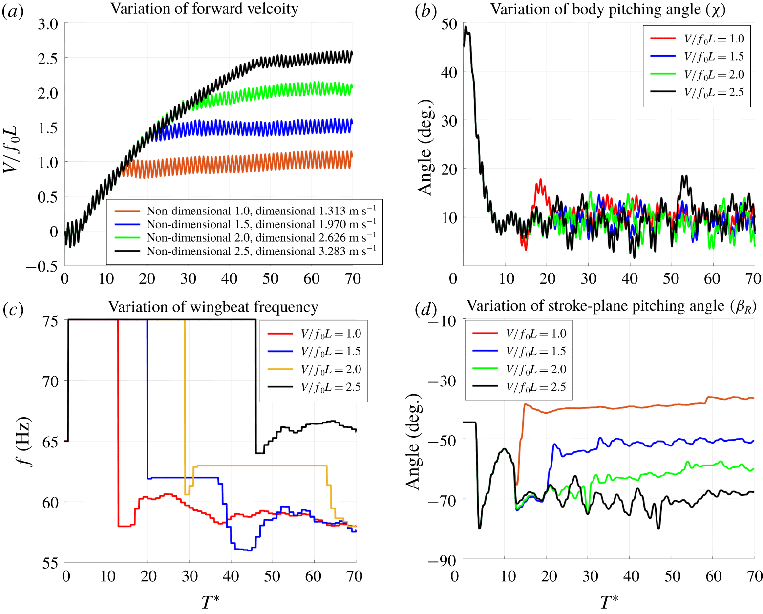
Variation of insect forward velocity (a), body pitching angle (b), wingbeat frequency (c) and stroke-plane pitching angle (d) during forward cruising flight at different speeds.

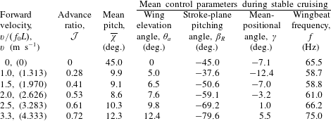
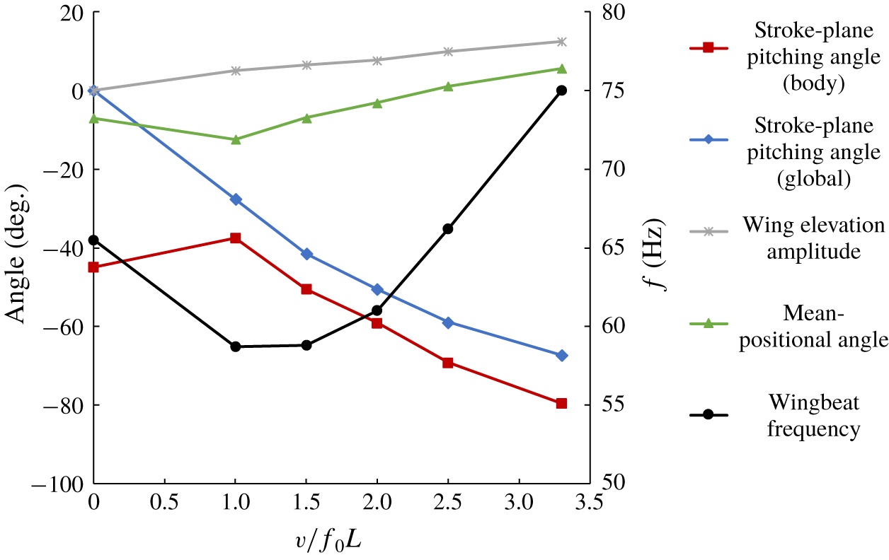
Variation of control parameters against non-dimensional forward speed  $v/(\,f_{0}L)$ during quasi-stable cruising flight.

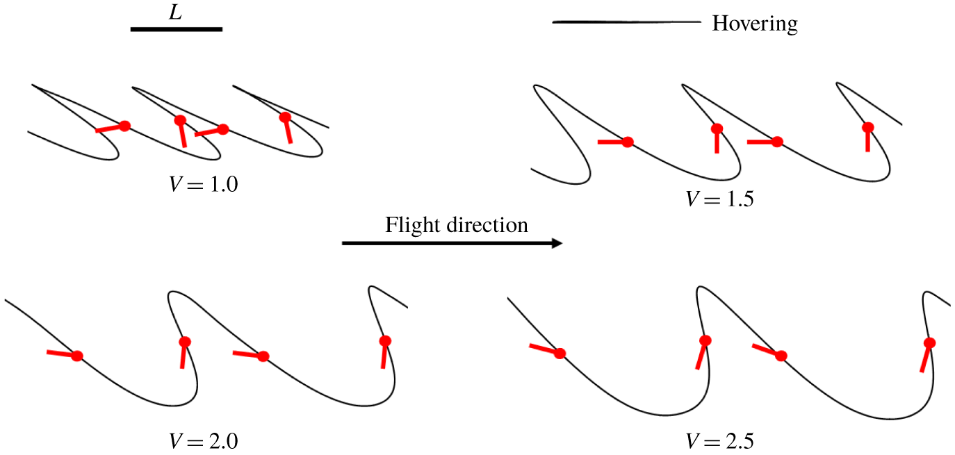
Wing-tip trajectories viewed in the global frame during forward cruising flight at different speeds. Red dots mark the leading edge of the wing chord. Unit wing length is represented by  $L$.

Four cruising flights were simulated, with cruising velocities ranging from  $1.0f_{0}L$ (
 $1.31~\text{m}~\text{s}^{-1}$) to
 $2.5f_{0}L$ (
 $3.28~\text{m}~\text{s}^{-1}$). These cases were achieved by switching control from acceleration mode to a speed-control mode when
 ${\sim}90\,\%$ of the desired cruising speed had been reached. The performance of the model hawkmoth in cruising flight is summarized in table 1 and figures 10 and 11 (including hovering flight), where the advance ratio is defined as
 ${\mathcal{J}}=v/(2\unicode[STIX]{x1D6F7}Lf)$, i.e. the ratio of insect forward velocity to the average wing-tip velocity. The model hawkmoth flies stably at the designated cruising speeds, during which the average body pitch angle is maintained at
 $\overline{\unicode[STIX]{x1D712}}\approx 10^{\circ }$ (figure 10b). The cessation of acceleration may be observed in figure 10(c), where the wingbeat frequency
 $f$ abruptly switches from 75 Hz to a lower value. During the cruising stage, the stroke-plane pitching angle (
 $\unicode[STIX]{x1D6FD}_{R}$) converges to a stable negative value with small fluctuations (see figure 10d). Cruising at a higher speed may be seen to require a more negative stroke-plane pitching angle (
 $\unicode[STIX]{x1D6FD}=\overline{\unicode[STIX]{x1D712}}+\unicode[STIX]{x1D6FD}_{R}$) for more of the wing force to be reoriented to the horizontal direction. The wingbeat frequency (
 $f$) shows similar converging behaviour, where the variations may be due to adjustments for height corrections. The height remains mostly within 0.5 wing length (
 $L$) of the initial height for the whole duration of flight – the deviations being small compared with the horizontal distance (from
 $65L$ to
 $110L$) traversed by the model hawkmoth. The lateral dynamics (roll, yaw and sideways motion) is similar to that in forward acceleration at constant
 $f=75~\text{Hz}$ (figure 9a,b). For all studied cases, roll/yaw angles are maintained within
 $\pm 2^{\circ }$ and lateral drifting does not exceed one wing length.
Figure 11 shows that the global stroke-plane angle  $\unicode[STIX]{x1D6FD}$ (figure 3b) becomes increasingly negative as the physical wing stroke plane tilts forwards to provide the necessary thrust to overcome a larger drag at a higher cruising speed. With the mean body pitch angle (
 $\overline{\unicode[STIX]{x1D712}}$) being uniformly maintained at
 ${\approx}10^{\circ }$ for all forward flights, this is achieved via changes in the relative stroke-plane angle (
 $\unicode[STIX]{x1D6FD}_{R}$) – the anomalous increase in
 $\unicode[STIX]{x1D6FD}_{R}$ for
 $v/(\,f_{0}L)$ from 0 to 1.0 is due to a sharp change in body pitch
 $\overline{\unicode[STIX]{x1D712}}$ from
 ${\sim}45^{\circ }$ for hovering to
 $10^{\circ }$. The wingbeat frequency
 $f$ goes through a decreasing–increasing trend as the forward speed increases from zero (hovering) – dropping to
 ${\sim}59~\text{Hz}$ for cruising speeds of
 $1.31{-}1.97~\text{m}~\text{s}^{-1}$ (
 $v/(\,f_{0}L)<1.5,{\mathcal{J}}<0.4$), before rising above the hovering frequency for
 $v>2.5~\text{m}~\text{s}^{-1}$ (
 ${\mathcal{J}}>0.6$), and thence to 75 Hz at the speed of
 $4.33~\text{m}~\text{s}^{-1}$. Such a U-shaped trend was observed in experiments by Dudley & Ellington (Reference Dudley and Ellington1990a), and also noted by others. To explain the fall below the hovering frequency, we note that, in normal hovering, the wing drag force largely cancels out over a complete wing cycle (due to the predominantly horizontal wing trajectory and stroke symmetry), and makes little or no direct contribution to the lift (net vertical force). In forward flight, the stroke asymmetry relative to the oncoming flow results in increased downstroke drag and reduced upstroke drag. The forward rotation of the wing stroke plane (trajectory inclined to the horizontal) then allows a component of the enhanced downstroke drag force to contribute directly to the vertical aerodynamic force. The energy expended to actuate the wings (against wing drag) is now more efficiently coupled to lift production; and a smaller wingbeat frequency is then required to generate the lift for cruising at low speed compared with purely hovering flight. Figure 11 shows that the increase in the cruising speed for
 $v>2~\text{m}~\text{s}^{-1}$ (see table 1) is driven by both an increase in wingbeat frequency
 $f$ and a decrease in the relative stroke-plane angle (
 $\unicode[STIX]{x1D6FD}_{R}$).
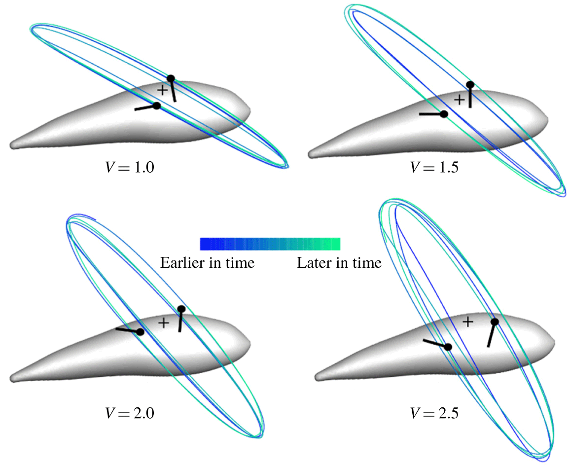
Figures 12 and 13 depict the wing-tip trajectories in the global and body frames, respectively, during quasi-stable cruising at various speeds. In both figures, the approximate wing chord is indicated with a dot on the leading edge to show the wing orientation. Figure 12 shows that the wing tip traces a longer path in the global frame in the downstroke than in the upstroke owing to the forward motion of the flyer. The upstroke tip trajectory, on the other hand, becomes more vertical with increase in the speed. In the body frame (figure 13), the wing-tip trajectories collapse to form a connected series of ‘oval-shaped’ loops. The conflated width and orientation of the loops reflect a mean elevation amplitude ( $\overline{\unicode[STIX]{x1D703}}_{a}$) and stroke-plane angle (
 $-\overline{\unicode[STIX]{x1D6FD}}$), respectively, that increase with the cruising speed of the flyer, which is consistent with earlier results.
Wing-tip trajectories (for  ${\sim}5$ wing cycles) viewed in the insect body frame during forward cruising flight at different speeds. Wing root is marked as (
 $+$).

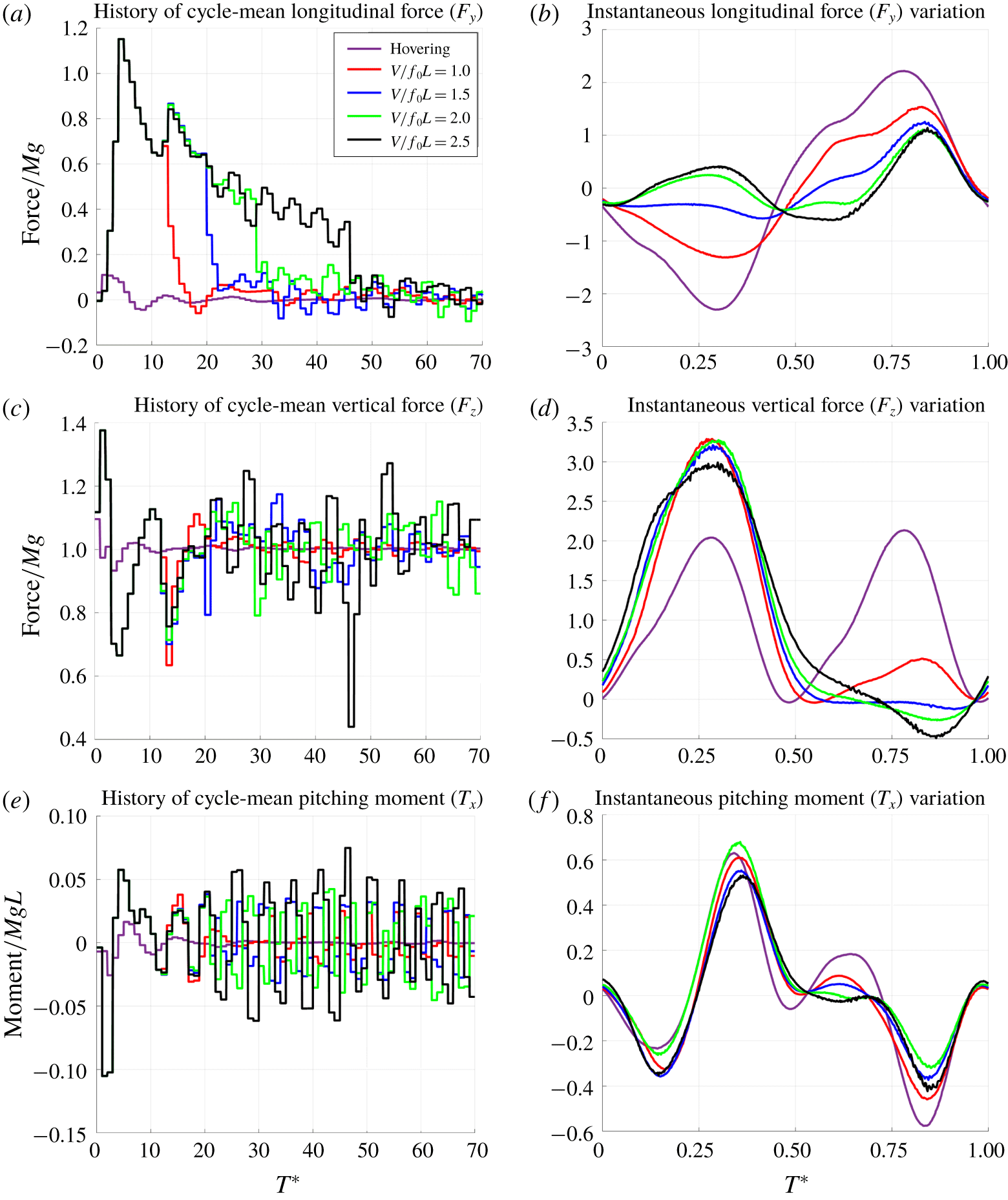
Comparison of aerodynamic forces and pitching moment for quasi-stable hovering and forward cruising flight at different cruising speeds. Histories of cycle-mean forces/moments (a,c,e) and instantaneous forces/moments (b,d,f) over the 61st wing cycle.

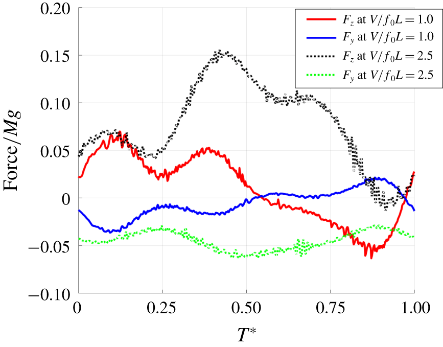
Comparison of aerodynamic longitudinal and vertical forces acting on the body of the model hawkmoth during forward cruising at different speeds.

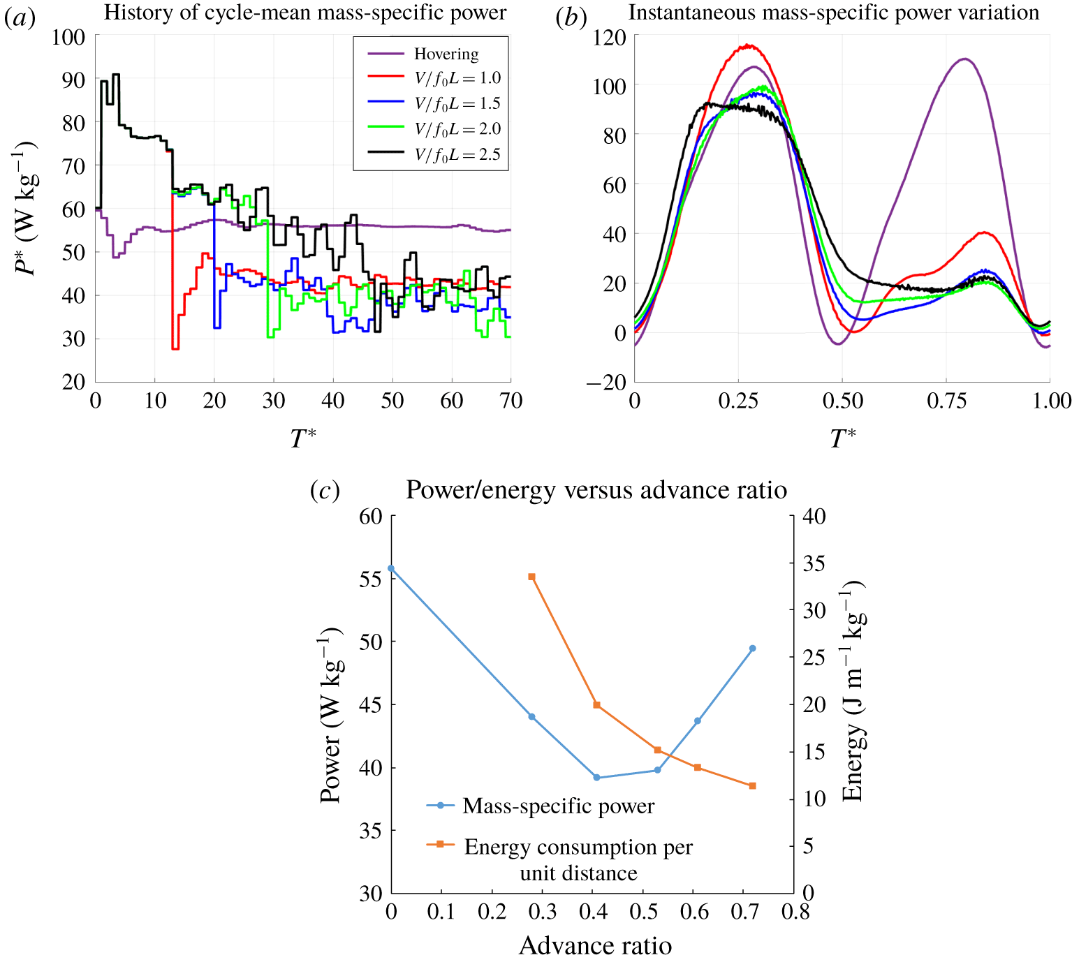
Aerodynamic power and energy consumption. (a) History of cycle-mean mass-specific power  $P^{\ast }$ (
 $\text{W}~\text{kg}^{-1}$), (b) instantaneous power over a wing cycle in equilibrium cruising, and (c) mean
 $P^{\ast }$ (
 $\text{W}~\text{kg}^{-1}$) and energy consumption (
 $\text{J}~\text{m}^{-1}~\text{kg}^{-1}$) in equilibrium cruising flight.

5.1.2 Forces, moments and power
Figure 14 shows the histories of cycle-mean and intra-cycle forces/moments for forward flights. The intra-cycle variations pertain to the 61st wing cycle, when the flyer is in quasi-equilibrium flight at the designated speeds. Figure 14(a) shows that the cycle-mean longitudinal force  $F_{y}$ drops abruptly to near zero when kinematic control is switched over from acceleration to cruising. The
 $F_{y}$ fluctuates with small deviations about zero during cruising. The cycle-mean vertical force (figure 14c) is poised near the weight of the model hawkmoth during the whole simulation, albeit with slightly larger fluctuations than corresponding longitudinal force. The fluctuations about the quasi-equilibrium values are larger than those in free hovering flight. The cycle-mean pitching moment also displays larger fluctuations (figure 14e) that increase roughly with the cruising speed – this is related to the amplitude of wing elevation
 $\unicode[STIX]{x1D703}_{a}$, which is linearly correlated with the speed of the flyer.
Figure 14(b) shows that the intra-cycle longitudinal force variation for quasi-steady forward flight deviates progressively from the hovering curve with increase in cruising speed  $v/(\,f_{0}L)$. Thrust (
 $F_{y}>0$) for forward motion is developed primarily in the upstroke at low to medium cruising speed to overcome drag present over the downstroke. However, a growing contribution to thrust is derived from the downstroke as cruising speed rises above 2, and drag shifts increasingly towards the late downstroke and early upstroke (where the longitudinal speed of the wings may be small relative to the oncoming flow). The intra-cycle vertical force variations in figure 14(d), on the other hand, show that the bulk of the vertical force during cruising is produced during the downstroke, with peaks rising well above the hovering value. The enhanced lifting force may be attributed to the inclined plunging trajectory of the wings during the downstroke (figure 12), indicating that aerodynamic drag on the wings is now beneficially exploited for enhanced lift generation. The upstroke contributes minimally to the overall lift; and a small negative lift may even occur at higher cruising speeds. The latter may be attributed to the steep trajectory of the upstroke, which veered close to the vertical at high cruising speed (figure 12) due to the large forward rotation of the stroke plane (
 $\unicode[STIX]{x1D6FD}\approx -59^{\circ }$ at
 $v=2.5f_{0}L$). With the accompanying rotation of the wing chord, the wing drag may then have a negative vertical component that is larger than the small (positive) vertical component of wing lift – resulting in a small net negative vertical wing force over a part of the upstroke. Figure 14(f) shows that the intra-cycle rise and fall of the pitching moments are surprisingly similar to each other, in both trend and magnitude, at all four cruising speeds and hovering.
Figure 15 shows the aerodynamic forces experienced by the body of the model hawkmoth (without the wings) over a wing cycle at the cruising speeds of  $1.0f_{0}L$ (
 $1.31~\text{m}~\text{s}^{-1}$) and
 $2.5f_{0}L$ (
 $3.28~\text{m}~\text{s}^{-1}$). It is evident that the body enjoys positive lift over virtually the entire wing cycle for its flight at the higher speed, which averages
 ${\sim}7\,\%$ of body weight over the wing cycle. This may be attributed to the favourable AoA (
 $\overline{\unicode[STIX]{x1D712}}\approx 10^{\circ }$) at which the body is poised. The high air speed also imposed a notable mean drag on the body that amounts to
 ${\sim}4\,\%$ of its weight. The lift gain is much smaller at the lower speed, due to both its reduced speed and the presence of a small negative lift over the upstroke (
 $0.5<T^{\ast }=tf<1.0$). Equally, the lower-speed case suffers lower body drag due to its lower speed and a weak thrust over its upstroke. The negative lift and weak thrust over the upstroke may be attributed to transient reduction in the pressure field below the fore body as the wing pair diverges at the start of the upstroke, and increased pressure above the aft body as the wings converges towards the end of the upstroke (see figure 13,
 $V=1.0$).
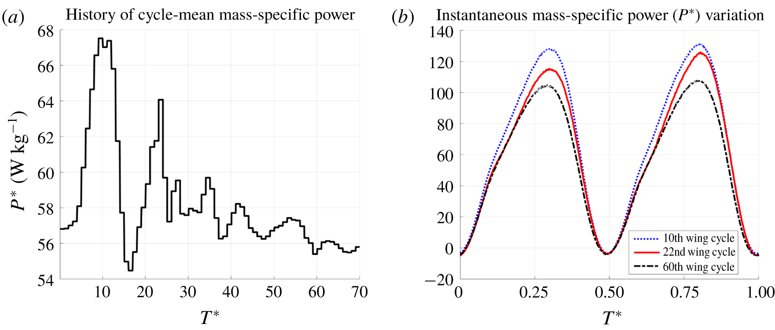
Aerodynamic power was computed by summing the rate of work done against aerodynamic forces over the whole surface of the model hawkmoth. Figure 16(a) shows that the cycle-mean aerodynamic power  $P^{\ast }$ (normalized by body mass) surges momentarily from
 ${\sim}56~\text{W}~\text{kg}^{-1}$ (hovering) to a high of
 ${\sim}90~\text{W}~\text{kg}^{-1}$ when the model hawkmoth is launched into accelerated flight at the wingbeat frequency of 75 Hz. The power falls rapidly thereafter as the flyer gained speed to eventually equilibrate approximately
 $40{-}50~\text{W}~\text{kg}^{-1}$ when control is changed over to cruising mode. The intra-cycle instantaneous aerodynamic power in figure 16(b) shows that the bulk of aerodynamic power is produced in the downstroke during steady cruising. This accords well with the larger aerodynamic force produced by the wings (figure 14b,d) and the longer distance (higher average speed) that they traversed in the downstroke (figure 12).
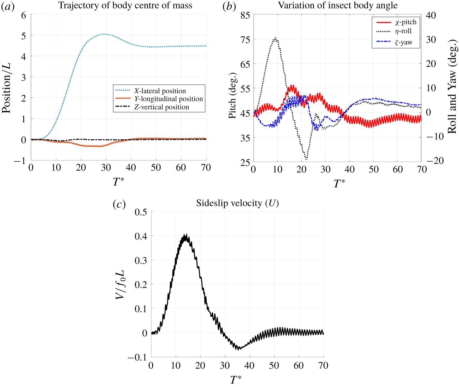
Variation of position, body angles and lateral velocity during sideslip manoeuvre.

Figure 16(c) presents the mean aerodynamic power for steady cruising flights as a function of advance ratio ( ${\mathcal{J}}$). It exhibits a decreasing–increasing trend, where the lowest power of
 ${\sim}40~\text{W}~\text{kg}^{-1}$ is recorded for
 ${\mathcal{J}}\sim 0.4{-}0.5$ (
 ${\sim}1.9{-}2.6~\text{m}~\text{s}^{-1}$). A significant rise in power (from
 $40~\text{W}~\text{kg}^{-1}$ to
 $49~\text{W}~\text{kg}^{-1}$) is also evident over the speed range,
 $0.5<{\mathcal{J}}<0.72$, where we had earlier noted a significant rise in the wingbeat frequency (table 1). Nevertheless, these rates are all below the mean hovering power of
 $56~\text{W}~\text{kg}^{-1}$ (
 ${\mathcal{J}}=0$). The comparative efficiency of cruising flights vis-à-vis hovering may be ascribed to the effective utilization of the wing drag force towards lift generation as noted earlier. It also suggests that the present hawkmoth may have energy headroom to go beyond the maximum cruising speed of
 $4.33~\text{m}~\text{s}^{-1}$ (
 ${\mathcal{J}}=0.72$) reached in this study. The falling-and-rising trend of the mean power curve in figure 16(c) is consistent with the U-shaped power curve predicted by the quasi-steady model of Pennycuick (Reference Pennycuick1975), and also observed in experiments on the bumblebee (Dudley & Ellington Reference Dudley and Ellington1990b) and hawkmoth (Willmott & Ellington Reference Willmott and Ellington1997b; Warfvinge, Kleinheerenbrink & Hedenström Reference Warfvinge, Kleinheerenbrink and Hedenström2017). Nevertheless, figure 16(c) also shows that the normalized energy cost per unit of distance travelled (
 $\text{J}~\text{m}^{-1}~\text{kg}^{-1}$) actually decreases monotonically with
 ${\mathcal{J}}$, indicating that higher speed may be beneficial for long-distance migration.
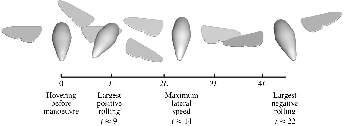
Sideslip manoeuvre in scaled physical space, viewed from the rear of the model hawkmoth, showing the displacement and posture of the flyer at different times, with wings poised at mid-downstroke.

5.2 Sideslip manoeuvre
In the current study, the model hawkmoth was directed to sideslip a distance of 4.5 wing lengths ( $L$) to its right and to hover with the same body orientation at the new position. Readers may refer to the supplementary movies for the animation of the sideslip manoeuvre.
5.2.1 Flight performance
The performance of sideslip manoeuvre is summarized in figure 17. It takes approximately 20 wing cycles for the model hawkmoth to traverse the distance of  $4.5L$ to reach its new position and another 25–30 wing cycles to re-establish hovering at the new location. Small overshoot in its lateral
 $x$ and longitudinal
 $y$ displacements may be observed (figure 17a), which are duly corrected by the 45th wingbeat during the re-hovering stage. The sideslip is motivated by
 $\unicode[STIX]{x1D6FF}_{SA}$-driven rolling of the body. The lateral velocity reaches its maximum value of
 $u/(\,f_{0}L)\sim 0.4$ at the 14th wing cycle (figure 17c) before it is arrested by a
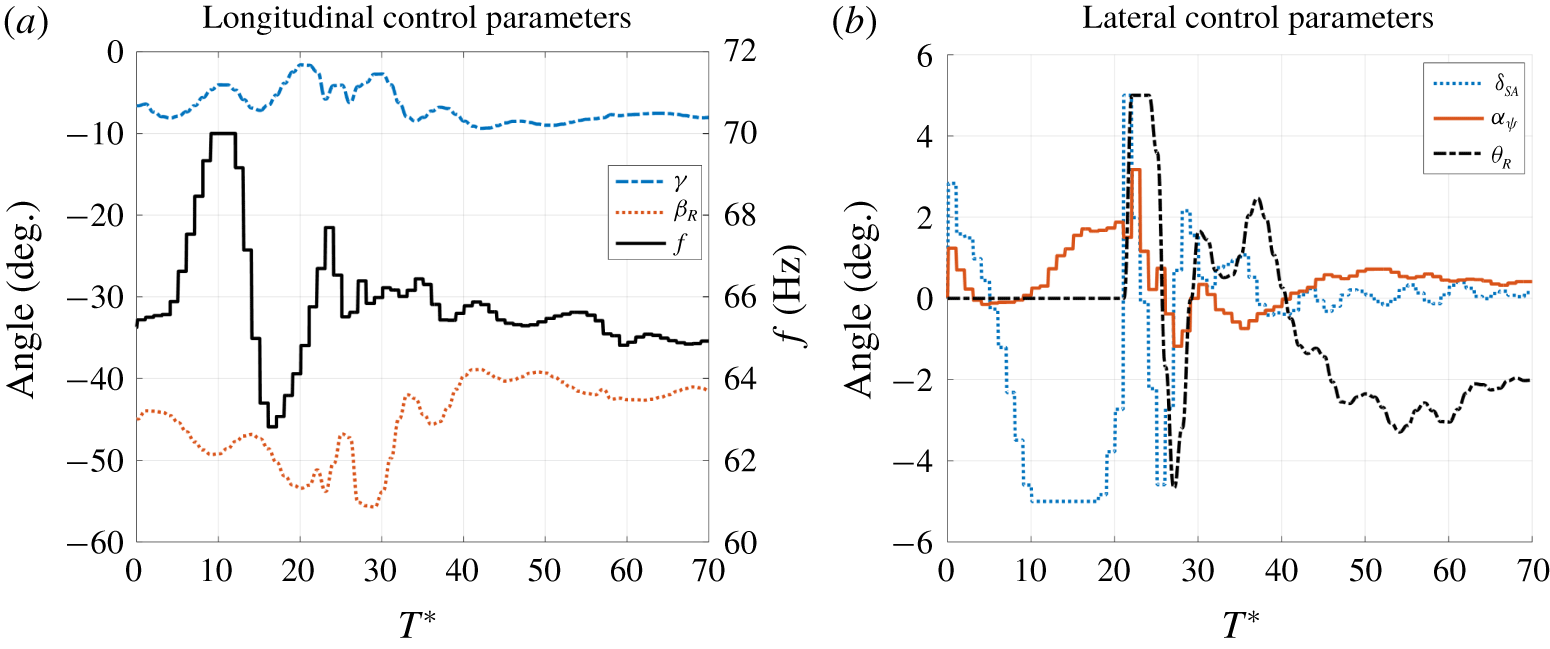
 $\unicode[STIX]{x1D6FF}_{SA}$-driven counter-rotation of the body – the rapid and large roll, and the sympathetic yaw of the flyer, may be seen in figure 17(b). Hovering control is reasserted from the 20th wing cycle, whereby the body roll is checked by the lateral rotation of the wing stroke plane (
 $\unicode[STIX]{x1D703}_{R}$). The execution of the manoeuvre in physical space is presented in figure 18, viewed from the rear of the flyer. Experiments by Greeter & Hedrick (Reference Greeter and Hedrick2016) showed the sideslip manoeuvre of a hawkmoth, M. sexta, that lasted for
 ${\sim}0.2~\text{s}$, which is comparatively close to the time in our simulation (20 wing cycles over
 ${\sim}0.3~\text{s}$). Their video clip shows that the hawkmoth took approximately 12 wing cycles to traverse approximately five wing lengths laterally (average speed
 ${\sim}0.4f_{0}L$) – wing cycles are counted where the flyer shows perceptible lateral movement. If we discount the first five or six wing cycles in the initialization of the sideslip manoeuvre (see figure 17a), which produces negligible lateral movement, only approximately 15 wing cycles are involved in the sideslip of the present hawkmoth over
 ${\sim}4.5$ wing lengths (average speed
 ${\sim}0.3f_{0}L$). Considering that M. sexta is a larger hawkmoth (
 $Re\sim 6000$), and the circumstances and motivation for the sideslip are different, the present results are quite reasonable.
Variation of longitudinal (a) and lateral (b) control parameters during sideslip manoeuvre.

Figure 19 shows the kinematic actions of the model hawkmoth during the manoeuvre. A portion of the wing lift is reoriented into the horizontal direction as the flyer rolls positively to accelerate and then negatively to decelerate itself into its new position. This inevitably leads to a momentary drop in the vertical force needed to support its weight. Responsive adjustments of the wingbeat frequency  $f$ (figure 19a) to amplify the wing force ameliorate the height drop to
 ${<}0.1L$ (figure 17a). The larger deviation in the longitudinal
 $y$ displacement of the flyer, on the other hand, may be attributed to the sympathetic yaw of the flyer attending the roll and counter-roll – which diverts a small component of the sideslip velocity into the global
 $y$-direction that causes the flyer to drift backwards initially and then forwards. Rolling and yawing of the flyer are dynamically coupled via the cross-component of body inertia (Yao & Yeo Reference Yao and Yeo2019c), so that an applied torque along one axis induces concomitant rotation along the other axis. Total variation of rolling angle (
 $\unicode[STIX]{x1D702}_{max}-\unicode[STIX]{x1D702}_{min}$) is
 ${\sim}50^{\circ }$ for the whole manoeuvre and fairly large rolling rate is observed. A maximum rolling rate of
 ${\sim}330^{\circ }~\text{s}^{-1}$ occurs during the deceleration stage. The variations of rolling angle and rolling rate are close to those observed by Greeter & Hedrick (Reference Greeter and Hedrick2016), which were approximately
 $50^{\circ }$ and
 $400^{\circ }~\text{s}^{-1}$, respectively. To achieve sufficient rolling moment for such a rapid roll, the stroke amplitude difference (
 $\unicode[STIX]{x1D6FF}_{SA}$) touches its lower bound in figure 19(b). Though essential control action was adopted for yaw control, it was not enough to fully eliminate the induced moment. Variations of pitch and yaw are nevertheless limited to approximately
 $\pm 10^{\circ }$ from their equilibrium values (figure 17b) during the sideslip manoeuvre.
5.2.2 Forces, moments and power
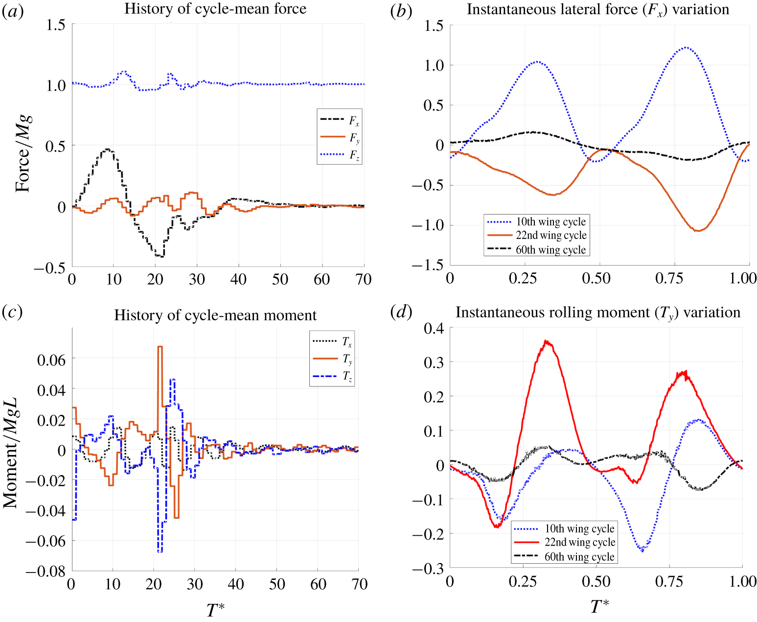
Figure 20 shows the history of forces and moments over the course of the manoeuvre and post-manoeuvre hovering. The variations of the cycle-mean forces/moments in figure 20(a,c) are consistent with the actions of control parameters in figure 19. Force variation occurs mainly in the lateral direction, which is consistent with the insect’s predominantly lateral motion during the manoeuvre. Unlike the hovering and forward flight, the pitching moment no longer dominates in a sideslip manoeuvre. Instead, rolling and yawing moments show larger variations (figure 20c), motivated by roll–yaw kinematic control action. Since lateral sliding and body rolling are the most significant components of motion during the sideslip manoeuvre, the intra-cycle variations of the lateral force ( $F_{x}$) and rolling moment (
 $T_{y}$) at different times in the manoeuvre are compared in figure 20(b,d). Positive lateral force and negative rolling moment are close to their peak in the 10th wing cycle (acceleration phase); while negative lateral force and positive rolling moment also reach their maximum in the 22nd wing cycle (deceleration phase). The peak lateral forces (
 $F_{x}$) in the 10th and 22nd cycles are roughly in antiphase. Lastly, results for the 60th wing cycle show reduced fluctuations and near-zero cycle mean of the lateral force and rolling moment, as the flyer approaches the quasi-equilibrium of re-established hovering at the new position.
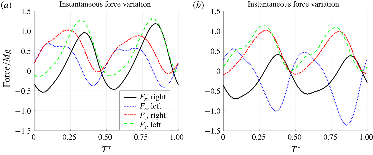
Lateral motion during sideslip implies that the cyclic lateral forces ( $F_{x}$) produced by the two wings are no longer in perfect antiphase as they were in hovering. Figure 21(a) shows that the lateral acceleration in the 10th wing cycle is led by lateral force (
 $F_{x}$) emanating from the left wing over the leading half of both its down- and upstrokes (first and third quarters), and lateral force from the right wing over the second half of the strokes (second and fourth quarters); with reinforcing thrusts from both wings around the mid-strokes (
 $T^{\ast }\approx 0.5$). The lifting forces (
 $F_{z}$) from the two wings are largely positive over the cycle to support the weight, but their relative shift in phase (
 ${\sim}30^{\circ }$) provides the negative rolling moment needed at this time when the body is near its point of maximum clockwise roll. These variations of the forces may be further explained to various extents by the changing relative velocity of the individual wings to the oncoming side flow over the different quarters of the wing cycle. Thus, lateral force on the right wing (vis-à-vis the left wing) was increased as it swept into the oncoming side flow in the first and third quarters; while its lift was compromised by adverse changes in the AoA of the relative airflow due to the highly rolled posture of the flyer. Similar deductions may be garnered from figure 21(b) for the 22nd wing cycle, with some differences in the details – with a smaller slip speed here, the lateral forces of the two wings become more antiphased and the lift forces more phase-aligned.
Aerodynamic force/moment variation: history of cycle-mean force/moment (a,c) and instantaneous force/moment variation within one wingbeat (b,d).

Aerodynamic force variation on left and right wings in (a) the 10th wing cycle and (b) the 22nd wing cycle.

Figure 22 shows the history of cycle-mean aerodynamic power over the manoeuvre and the instantaneous variations over a wing cycle at different flight stages. The variation of the cycle-mean power is closely allied to the variation of wingbeat frequency (figure 19a), i.e. more power is required at higher frequency and vice versa. The power consumption during the sideslip manoeuvring proper ( $0<T^{\ast }<30$) is generally higher than that in quasi-equilibrium hovering, because more wing lift had to be generated to balance the body weight during body rolls. A similar trend is observed for intra-cycle power variations at the different flight stages, with one peak for each stroke (figure 22b).
Aerodynamic power variation during sideslip manoeuvre: (a) history of cycle-mean power variation and (b) instantaneous power variation over one wing cycle.

Vortex wake during transition from hovering to forward acceleration (side view),  $\unicode[STIX]{x1D706}_{2}=-10$. (a) Hovering before transition, (b) the second wing cycle after transition, (c) the fourth wing cycle after transition, and (d) the sixth wing cycle after transition.

6 Flow aspects
6.1 Forward flight
Figure 23 shows the evolution of the vortex wake during the transition from hovering flight to forward acceleration. Figure 23(a) shows the vertically layered vortex wake produced by the horizontally reciprocating motion of the wings in normal hovering. When forward flight is initiated, the rapidly steepening stroke of the wings begins to ‘cut’ into the existing vortical stack below the flyer. The complex reconfiguration of the vortex wake (figure 23b,c) that follows results in a forward-tilted layered wake (figure 23d), which becomes increasingly evident and distinct as the flyer displaces forwards.
The vortices created by the sweeping wing of an insect in flight typically comprises the leading-edge vortex (LEV), the wing-tip vortex (WTV) and the trailing-edge vortex (TEV) – these being identified by the regions on the wing where they emanated (and visualized here by their  $\unicode[STIX]{x1D706}_{2}$ isosurfaces). In forward flight, where the wing may be subject to a significant oncoming airflow, vorticity shed from the inner edge of the wing (adjacent to the body) may form a distinct vortex (from the TEV) that may be termed the wing-root vortex (WRV). These vortices are created at the start of a wing stroke. The buildup of vorticity in the LEV and TEV is drained progressively from the wings via the WTV and WRV during the wing stroke. These vortices detach from the wing in the form of a connected vortex loop (loosely termed a ring) towards the end of the stroke. From the midst of the LEV and TEV that are shedding from the wing towards the end of the stroke, a new nascent system of LEV–WTV–TEV–WRV (see figure 24) emerges on the reversing wing, and a new wing cycle commences. The sectional plot of the flow velocity vector (figure 24d) shows clearly strong downwash created by the downstroke and the backward jet by the upstroke. The upstroke also produces a smaller downwash that contributed to the lift (at this cruising speed), while the downstroke also incurred drag that was balanced by the thrust of the forward jet during equilibrium forward flight. These are consistent with the cyclic wing force variations depicted in figure 14(b,d). Similar repetitive vortical structures were also observed in the wake flow of butterfly (Brodsky Reference Brodsky1991) and hawkmoth (Willmott, Ellington & Thomas Reference Willmott, Ellington and Thomas1997) in tethered flights. Limitations of experimental techniques have hitherto only permitted sectional views of the wake to be directly visualized; whereas CFD simulation allows one to capture a more comprehensive picture of vortex formation and evolution.
Vortex wake for forward cruising flight at speed  $v=1.0f_{0}L$,
 $\unicode[STIX]{x1D706}_{2}=-10$, frequency
 $f\approx 59~\text{Hz}$.

Vortex wake of forward flight at  $v=1.5f_{0}L$,
 $\unicode[STIX]{x1D706}_{2}=-10$.

Vortex wake of forward flight at  $v=2.5f_{0}L$,
 $\unicode[STIX]{x1D706}_{2}=-10$.

Vortex wake of hovering flight at time  $t=0.25$ upon the initiation of sideslipping: (a,b) show the overall vortex formation: (c,d) the leading vortex structures around wings.

Vortex wake in sideslip manoeuvre at the time ( $t=9.25$) of maximum body roll: (a,b) show the overall vortex formation; (c,d) the leading vortex structures around the wings.

Vortex wake in sideslip manoeuvre at the time ( $t=14.25$) of maximum lateral speed: (a,b) show the overall vortex formation, (c,d) the leading vortex structures around the wings.

Vortex wake in sideslip manoeuvre at the time ( $t=22.25$) of largest negative body roll: (a,b) show the overall vortex formation, (c,d) the leading vortex structures around the wings.

In hovering flight, shed vortices in the wake are typically arranged in two fairly distinct vertically aligned vortical stacks, one below each wing (figures 23a and 27). In slow longitudinal flight, these vortical columns lean forwards in the direction of flight owing to the motion of the flyer. Vortical details within the wake are highly complex, especially at low speed, as vortices shed in close proximity to each other often intertwine and weave into each other under their mutually induced velocity field. Moreover, overlap in the sweep volumes of a wing may also occur (see tip trajectory in figure 12), thus causing nascent growing vortices in the downstroke to interact directly with the already shed vortices of the preceding upstroke. The shed vortex loops may assume a ring-like appearance upon shedding from the wing; with rings from consecutive strokes linked to each other via weaker vortical strands. At higher forward speed, vortices from consecutive strokes are shed further apart, thus reducing their interaction, and making it easier for an observer to discern their formation.
Figure 25 shows the vortex wake behind the model hawkmoth in accelerating and cruising flight at the speed of  $v=1.5f_{0}L$, where the shed vortex loops/rings of the downstrokes (VR-D
 $x$) and upstrokes (VR-U
 $x$) are identified – the number
 $x$ denotes that it was shed by the
 $x$th preceding stroke relative to the current wing stroke. One may also observe that the downstroke rings VR-D
 $x$ at
 $v=1.5f_{0}L$ are roughly aligned horizontally, whereas the upstroke rings are poised more towards the vertical. This is consistent with the production of down jets by the downstrokes as the primary lift-producing strokes in the wing cycle (figure 14d) during forward flight; whilst generation of thrust is accomplished by backward jets set up by the upstrokes (figure 14b). The downstroke rings assume a more longitudinally stretched appearance at the higher speed of
 $2.5f_{0}L$ in figure 26, plus a forward tilt that recalls the positive thrust that develops over the downstrokes at this speed in figure 14(b). Figures 25 and 26 show that vortices from consecutive strokes are shed closer to each other during acceleration than in cruising at the same speed – this may be accounted for by the higher wingbeat frequency of the former. The body-shed vortex (BdV) in figures 25 and 26 denotes weak vortices shed from the body of the flyer, which may be associated with cyclic fluid forces acting on the body. BdVs were observed by Liu, Dong & Li (Reference Liu, Dong and Li2016) in a study of cicada flight, and by Yao & Yeo (Reference Yao and Yeo2018) in their simulation of a free-flying fruit fly.
6.2 Sideslip manoeuvre
Figures 27–30 show the vortical wakes at four time instants in the sideslip manoeuvre of the model hawkmoth that correspond to the flight sequence depicted in figure 18. From its initial hovering posture ( $t=0.25$, figure 27) with the symmetric wake, the wake sways to the left as the flyer rolls rapidly and drifts to its right during the acceleration phase of the manoeuvre to reach its maximum-rolled posture at time
 $t=9.25$ in figure 28. The left bias of the momentum jet created by the left wing (figure 28c) confirms the lateral-force dominance of the left wing noted earlier in figure 21(a) (
 $T^{\ast }=0.25$). The model insect is translating at maximum lateral speed
 $u_{max}$, with a distinctive left-trailing wake, at
 $t=14.25$ in figure 29. It recovers a nearly upright body posture by this time, but is still counter-rolling at a high anticlockwise rate. These combine to reduce the AoA of the flow near the tip region of the right wing, leading to reduced force production that is manifested by the expansion of the LEV core there (figure 29c,d); the reverse is applicable for the left wing.
In insect flight, vortex formation is largely dominated by the mechanism of lift production, and lateral force production may amount to only a small bias of the principal events ( $u_{max}/V_{tip}\approx 0.4/5.4$ here). This, on top of other reasons already given for intensive vortex interactions, makes the vortical events appertaining to sideslip difficult to isolate. Finally, figure 30 shows the model hawkmoth at maximum negative body roll, as it attempts to slow down its lateral drift to hover at the new designated location. Here one may observe, in contrast to figure 29, the ‘warping’ of the vortical wake columns below each of the wings produced by the negative rolling of the flyer, as well as the ‘swaying’ of the wake columns back to the right. The slightly expanded core of the LEV near the tip of the right wing (figure 30c,d) also suggests reduced suction, and hence lift, on the right wing vis-á-vis the left wing, which is borne out in figure 21(b) (at mid-downstroke).
7 Concluding summary
The present work is an attempt to computationally simulate the longitudinal free flight and the sideslip manoeuvre of a model hummingbird hawkmoth, which has a wing-flapping Reynolds number  $Re\sim 3000$. The computational model integrated a Navier–Stokes fluid solver with the six-degree-of-freedom Newtonian free-body dynamics of the model insect and a generic PID-based controller for wing kinematics to achieve stable directed free flight. It is the first time that free flights have been investigated numerically by such an inclusive approach for a relatively large insect. Comprehensive state-equation analyses on the flyer dynamics and control strategies for both forward flight and sideslip manoeuvre were presented. The reduced form of the state-equation models can be helpful in establishing the kinematic control coefficients needed for stable flight, when combined with a suitable wing force model (Yao & Yeo Reference Yao and Yeo2019b). The entire process of both flight modes was simulated in ‘real time’ under dynamic active flight control, where the physics at different stages of the flight was investigated, i.e. from acceleration to constant-speed cruising for the forward flight, and from lateral rolling to re-hovering for the sideslip manoeuvre.
A set of prescribed-motion simulations was first conducted to evaluate the derivatives for force/moment variation against insect (translational and angular) speeds, which were helpful for establishing the kinematic control coefficients for a stable flight controller. Accelerating longitudinal flight at fixed wingbeat frequency of  $f=75~\text{Hz}$ was first simulated, where the model hawkmoth was rapidly pitched forward by a combination of elevation-induced aerodynamic and wing-mass-induced inertia pitching moment. The model hawkmoth achieved a near-equilibrium speed of
 $4.33~\text{m}~\text{s}^{-1}$ (advance ratio
 ${\mathcal{J}}=0.72$) at the end of 150 wing cycles, which is fairly close to the maximum of
 $4.86~\text{m}~\text{s}^{-1}$ estimated from the prescribed-motion study. Cruising flights with speeds of up to
 $3.28~\text{m}~\text{s}^{-1}$ (
 ${\mathcal{J}}=0.61$) were simulated. Wing elevation played an important role here in the control of cruising flight to surmount the strong pitching-up moment that the model hawkmoth encountered in forward flight. The bulk of the lift for forward flight was produced during the downstrokes. Thrust was produced by the upstrokes at low to medium speed, with downstrokes also contributing to thrust at higher speeds. The body also enjoyed a mean lift and drag amounting to 7 % and 4 % of body weight, respectively, at the speed of
 $3.28~\text{m}~\text{s}^{-1}$. The study indicates that the wingbeat frequency (
 $f$) for constant-speed cruising was generally lower than that for hovering flight in the low- and medium-speed range, before rising to higher values at higher speeds.
In a similar vein, aerodynamic power (body-mass-specific) also decreased with rise in cruising speed from  $56~\text{W}~\text{kg}^{-1}$ at hovering to
 ${\sim}40~\text{W}~\text{kg}^{-1}$ at
 $1.97~\text{m}~\text{s}^{-1}$ before rising back up to
 $49~\text{W}~\text{kg}^{-1}$ at
 $4.33~\text{m}~\text{s}^{-1}$. The reduced power may be attributed to the effective utilization of wing drag towards overall lift generation. This decreasing–increasing aerodynamic power trend is consistent with what several researchers have reported in the literature (Pennycuick Reference Pennycuick1975; Dudley & Ellington Reference Dudley and Ellington1990b; Willmott & Ellington Reference Willmott and Ellington1997b; Warfvinge et al. Reference Warfvinge, Kleinheerenbrink and Hedenström2017). In addition, higher-speed flights were more efficient in terms of distance travelled per unit of energy consumed – which hence favours migratory flight. The vortex wake behind the model hawkmoth comprised a symmetric pair of streaming vortex rings, where the downstroke-shed rings (associated with down-jets for lift) were oriented roughly horizontally, whereas the weaker and less distinct upstroke-shed rings (associated with backward jets for thrust) were aligned towards the vertical. The wake streams were fairly similar for constant-speed cruising and accelerating flight at the same speed, except for the slightly closer interval of the shed rings for the latter, due to its higher wingbeat frequency.
A sideslip manoeuvre was also simulated in which the model hawkmoth flew laterally to hover at a new location 4.5 wing lengths to its right. The simulation was preceded by a prescribed-motion study to determine the stability derivatives involved in sideways motion. The manoeuvre was accomplished by rolling the hawkmoth to its right to generate the requisite lateral force for sideslip, and then counter-rolling to decelerate and eventually re-establish hovering at the new location. The flyer took approximately 20 wing cycles to cover the designated distance and another approximately 30 wing cycles to re-stabilize hovering at the new location. The wingbeat frequency and aerodynamic power increased briefly during the manoeuvre to correct for the momentary fall in the lift caused by rolling. The manoeuvre time, maximum body roll angle and roll rate are compatible with published results for a comparable insect. The vortical wake swayed to the left as the model hawkmoth drifted to its the right. The wakes generated by the two wings, however, remain fairly distinct and separate throughout the manoeuvre. The changing disposition of the LEVs on the individual wings fairly reflects the varying lift on the wings at key stages of the manoeuvre.
Declaration of interests
The authors report no conflict of interest.
Supplementary movies
Supplementary movies are available at https://doi.org/10.1017/jfm.2020.361.
Appendix A. Table of variables/parameters

Appendix B. Coupled fluid–body solver
The fluid flow around the model insect is governed by the 3-D incompressible Navier–Stokes equations, in the non-dimensional arbitrary Lagrangian–Eulerian (ALE) form given here:
 $$\begin{eqnarray}\left.\begin{array}{@{}c@{}}\unicode[STIX]{x1D735}\boldsymbol{\cdot }\boldsymbol{u}=0,\\ \unicode[STIX]{x2202}_{t}\boldsymbol{u}=-(\boldsymbol{u}-\boldsymbol{u}^{g})\boldsymbol{\cdot }\unicode[STIX]{x1D735}\boldsymbol{u}+{\displaystyle \frac{1}{\mathit{Re}}}\unicode[STIX]{x1D6FB}^{2}\boldsymbol{u}-\unicode[STIX]{x1D735}p,\end{array}\right\}\end{eqnarray}$$
where  $\boldsymbol{u}$ and
 $p$ represent the velocity and pressure fields of the fluid domain, respectively. The
 $\boldsymbol{u}^{g}$ is the convection velocity of the computational node, which is equal to zero for stationary nodes. A projection-based method is adopted to solve the above equations, where the insect body and wings are modelled as non-slip surfaces
 $\unicode[STIX]{x1D6E4}(t)$, on which
 $\boldsymbol{u}(\boldsymbol{x})=\boldsymbol{u}^{g}(\boldsymbol{x})$. The pressure boundary condition is given by
 $\boldsymbol{n}\boldsymbol{\cdot }\unicode[STIX]{x1D735}p=-\boldsymbol{n}\boldsymbol{\cdot }\boldsymbol{a}$, where
 $\boldsymbol{a}$ is the acceleration of the surface node. Neumann-type boundary conditions are applied at the far-field boundaries of the flow domain. Temporal discretization of the governing equations is based on the implicit second-order Crank–Nicolson (CN) scheme. The flow equations are solved on a hybrid mesh consisting of background Cartesian nodes and clouds of mesh-free nodes around immersed boundaries. Different spatial discretization schemes are applied according to the type of the computation nodes. The standard seven-point central finite difference scheme is applied at Cartesian grid nodes that do not have mesh-free nodes nearby, while the singular value decomposition–generalized finite difference (SVD-GFD) scheme is applied at the mesh-free nodes and Cartesian nodes with mesh-free nodes nearby. Solutions by this scheme have been discussed in detail by Chew, Yeo & Shu (Reference Chew, Yeo and Shu2006), Wang et al. (Reference Wang, Yeo, Chew and Khoo2008, Reference Wang, Yu, Yeo and Khoo2010), Yu et al. (Reference Yu, Yeo, Shyam Sundar and Ang2011) and Zhang (Reference Zhang2013). The configuration of the nodal mesh around the model hawkmoth is shown in figure 31(a). A uniform Cartesian background grid had been adopted for the domain – figure 31(b) gives a partial view to highlight the placement of the model fly.
Grid system for numerical simulation. (a) Clouds of mesh-free nodes around the model flyer. (b) Partial view of the hybrid mesh consisting of Cartesian grids and mesh-free nodes.

The free flight of the model insect is governed by Newtonian dynamics. Assuming the body and wings to be essentially rigid, the kinematic and dynamic equations for flight are given by
 $$\begin{eqnarray}\displaystyle & \displaystyle {\displaystyle \frac{\text{d}}{\text{d}t}}\boldsymbol{X}_{B}(t)=\boldsymbol{V}_{B}(t), & \displaystyle\end{eqnarray}$$
 $$\begin{eqnarray}\displaystyle & \displaystyle {\displaystyle \frac{\text{d}}{\text{d}t}}\unicode[STIX]{x1D723}(t)=[\unicode[STIX]{x1D646}(\unicode[STIX]{x1D723})]\unicode[STIX]{x1D74E}(t), & \displaystyle\end{eqnarray}$$
 $$\begin{eqnarray}\displaystyle & \displaystyle {\displaystyle \frac{\text{d}}{\text{d}t}}(m_{B}\boldsymbol{V}_{B}+m_{lw}\boldsymbol{v}_{lw}+m_{rw}\boldsymbol{v}_{rw})=-M\boldsymbol{g}+\boldsymbol{F}_{A}, & \displaystyle\end{eqnarray}$$
 $$\begin{eqnarray}\displaystyle & \displaystyle {\displaystyle \frac{\text{d}}{\text{d}t}}(\boldsymbol{L}_{B}^{C}+\boldsymbol{L}_{lw}^{C}+\boldsymbol{L}_{rw}^{C})=\boldsymbol{T}_{A}^{C}. & \displaystyle\end{eqnarray}$$
 $\boldsymbol{X}_{B}(t)$ and
 $\boldsymbol{V}_{B}(t)$ are the position and velocity of the insect-body CoM at time
 $t$;
 $\unicode[STIX]{x1D723}(t)$ is the orientation vector of the flyer;
 $[\unicode[STIX]{x1D646}(\unicode[STIX]{x1D723})]$ is the transformation matrix relating the rate of change of
 $\unicode[STIX]{x1D723}(t)$ to the angular velocity
 $\unicode[STIX]{x1D74E}(t)$ of the body;
 $m_{B}$,
 $m_{\mathit{lw}}$ and
 $m_{\mathit{rw}}$ denote the mass of the insect body, and the left and right wings, respectively; and
 $\boldsymbol{v}_{\mathit{lw}}$ and
 $\boldsymbol{v}_{\mathit{rw}}$ are the corresponding velocities of the wings’ centres (of mass). The
 $\boldsymbol{L}_{B}^{C}$ denotes the angular momentum of the body about the whole insect’s CoM at
 $\boldsymbol{X}_{C}(t)$; and the
 $\boldsymbol{L}_{\mathit{lw}}^{C}$ and
 $\boldsymbol{L}_{\mathit{rw}}^{C}$ denote the same for the left and right wings, respectively. The closed-form expressions for these vectorial terms are rendered highly complex because of the intricate kinematics of the two wings, plus the relative shifting of the insect’s CoM within the body frame during wing flapping. The reader is referred to Yao (Reference Yao2018) for their derivation and further details.
Lastly, the  $\boldsymbol{F}_{A}(t)$ and
 $\boldsymbol{T}_{A}^{C}(t)$ denote the net resultant aerodynamic force and moment, respectively, acting on the flyer about
 $\boldsymbol{X}_{C}$, which are calculated as follows:
 $$\begin{eqnarray}\left.\begin{array}{@{}c@{}}\boldsymbol{F}_{A}(t)=\displaystyle \int _{\unicode[STIX]{x1D6E4}(t)}\unicode[STIX]{x1D748}\boldsymbol{\cdot }\boldsymbol{n}\,\text{d}\unicode[STIX]{x1D6E4},\\ \boldsymbol{T}_{A}^{C}(t)=\displaystyle \int _{\unicode[STIX]{x1D6E4}(t)}(\boldsymbol{x}-\boldsymbol{X}_{C}(t))\times (\unicode[STIX]{x1D748}\boldsymbol{\cdot }\boldsymbol{n})\,\text{d}\unicode[STIX]{x1D6E4},\end{array}\right\}\end{eqnarray}$$
where  $\unicode[STIX]{x1D748}=-p\unicode[STIX]{x1D644}_{identity}+(1/\mathit{Re})[\unicode[STIX]{x1D735}\boldsymbol{u}+(\unicode[STIX]{x1D735}\boldsymbol{u})^{\text{T}}]$ is the Newtonian fluid stress tensor derived from the flow solver;
 $\boldsymbol{x}$ is the location of a point on the surface; and
 $\boldsymbol{n}$ is the outer normal vector at
 $\boldsymbol{x}$. The integral is carried out over the surface configuration
 $\unicode[STIX]{x1D6E4}(t)$ of the flyer at time
 $t$.
Rolling rotation of wing frame/stroke plane, defined by angle  $\unicode[STIX]{x1D703}_{R}$, viewed from the rear of the insect.

Definition of the mean-positional angle, i.e. yawing rotation of wing frame. This shows a schematic drawing of the wing stroke plane viewed from the top.

The dynamics equations (B 2a–d) are discretized and integrated in time with the same CN scheme as the flow-field calculations. The integration of (B 2a–d) in time requires the concurrent solution of the flow field, while the motion of the model insect determines the solid boundary conditions for the flow solver. Hence, the use of the implicit CN scheme implies the need to iterate the solution process between flow solver  $\boldsymbol{F}[\unicode[STIX]{x1D6E4}(t)]$ and the body dynamic solver
 $\boldsymbol{S}\{\boldsymbol{F}[\unicode[STIX]{x1D6E4}]\}$ of (B 2) at each time step to determine the updated/new configuration of the flyer
 $\unicode[STIX]{x1D6E4}(t)$. The resultant fluid–body interaction problem to determine the configuration
 $\unicode[STIX]{x1D6E4}(\boldsymbol{G}(t)\mid t,\boldsymbol{X}_{\mathit{B}},\unicode[STIX]{x1D723},\boldsymbol{V}_{B},\unicode[STIX]{x1D74E})$ of the flyer at time
 $t$, where
 $\boldsymbol{G}(t)$ denotes the kinematic actions of the wings, may be symbolically represented by the process equation
 $\unicode[STIX]{x1D6E4}(t)=\boldsymbol{S}\{\boldsymbol{F}[\unicode[STIX]{x1D6E4}(t)]\}$, which has the form of a fixed-point problem. The iteration is carried out at each time step until the change between consecutive estimates of
 $\unicode[STIX]{x1D6E4}$ is smaller than a given tolerance. This procedure has been discussed and validated by Yeo, Ang & Shu (Reference Yeo, Ang and Shu2010) and Yu et al. (Reference Yu, Yeo, Shyam Sundar and Ang2011), and applied by Wu et al. (Reference Wu, Yeo and Lim2014) and Yao & Yeo (Reference Yao and Yeo2018) in free-flight studies.
Variation of the wing-twist angle  $\unicode[STIX]{x1D713}(t)$ with AoA
 $\unicode[STIX]{x1D6F9}_{M}+\unicode[STIX]{x1D6FC}_{\unicode[STIX]{x1D713}}$ at mid-stroke downstroke and
 $\unicode[STIX]{x1D6F9}_{M}-\unicode[STIX]{x1D6FC}_{\unicode[STIX]{x1D713}}$ at mid-stroke upstroke.

Appendix C. Kinematic control parameters
The additional flight control parameters used in the current study are summarized in this appendix. The rolling rotation (about the  $y^{w}$-axis) of the stroke plane contributes lateral force (
 $x$-direction) for correcting the left/right motion, and this rotation is denoted by
 $\unicode[STIX]{x1D703}_{R}$ (see figure 32). Similarly, the yawing rotation (about the
 $z^{w}$-axis) of the wing frame leads to the bias of wing stroking action forwards (ventrally) or backwards (dorsally) with respect to the insect body. This rotation is measured by the mean position angle
 $\unicode[STIX]{x1D6FE}$, the definition of which is shown in figure 33. Bias of the stroking action forwards or backwards via
 $\unicode[STIX]{x1D6FE}$ shifts the centre of the cycle-mean wing force to generate the desired pitching moment on the flyer. In addition, asymmetric wing motion, as an intra-stroke mode of adjustment, can be used to produce bilateral asymmetric moments to achieve roll/yaw control. In the present study, rolling moment is generated by differentially varying the lift forces of the two wings. Insects usually implement this mechanism for rapid turning in nature, which is achieved by decreasing the stroke amplitude (
 $\unicode[STIX]{x1D6F7}$) of one wing while increasing that of the other simultaneously, by a small adjustment
 $\pm \unicode[STIX]{x1D6FF}_{SA}$. Mean force along the stroke plane can be varied by applying different wing twist angles (
 $\unicode[STIX]{x1D713}$) to the two wings. This is done by adjusting the mid-stroke AoA of the two wings via
 $\unicode[STIX]{x1D6FC}_{\unicode[STIX]{x1D713}}$. As shown in figure 34, the wing initially flaps with mid-AoA
 $\unicode[STIX]{x1D6F9}_{M}$ for both downstroke and upstroke. If the AoA is changed to (
 $\unicode[STIX]{x1D6F9}_{M}+\unicode[STIX]{x1D6FC}_{\unicode[STIX]{x1D713}}$) for the downstroke, and to (
 $\unicode[STIX]{x1D6F9}_{M}-\unicode[STIX]{x1D6FC}_{\unicode[STIX]{x1D713}}$) for the upstroke, a negative mean force along the stroke plane can be produced. If the mid-AoA is changed asymmetrically for the two wings, a pair of forces in opposite directions is generated, which sets up a yawing moment. For current study, the adjustment of
 $\unicode[STIX]{x1D6FC}_{\unicode[STIX]{x1D713}}$ is used for yawing moment control.