2. Formulation

Consider a dusty plasma embedded in a constant magnetic field $\boldsymbol{B}_{0}=B_{0}\hat{z}$ , where $B_{0}$ is the strength of the ambient magnetic field along the $z$ direction. The gradients in the density [ $\boldsymbol{{\rm\nabla}}n_{d_{0}}(x)$ ] are along the negative $x$ -axis. Both the electrons and ions are modelled with a Lorentzian or kappa distribution, which has been successfully applied to non-equilibrium systems (Dovner et al. Reference Dovner, Eriksson, Bostrom and Holback1994; Cairns et al. Reference Cairns, Mamun, Bingham, Bostrm, Dendy, Nairn and Shukla1995; Hellberg & Mace Reference Hellberg and Mace2002). The satellite measurements of space plasmas clearly show the existence of particles that are far away from a thermodynamical equilibrium. The well known Maxwellian distribution is not appropriate for the description of such non-equilibrium plasma systems. Space plasmas e.g. solar wind, terrestrial magnetospheres and interstellar medium contain a significant population of superthermal particles and are examples of the non-Maxwellian plasmas (Montgomry, Bame & Hundhause Reference Montgomry, Bame and Hundhause1968; Vasylunais Reference Vasylunais1968). This distribution has been used to a great extent in both space and laboratory plasmas.

The kappa distribution can be written as,

where ${\it\kappa}$ is the spectral index which determines the deviation from a Maxwellian distribution. In a limiting case, when Kappa approaches to infinity ( ${\it\kappa}\rightarrow \infty$ ), the superthermal distribution reduces to the Maxwell–Boltzmann distribution. The symbol ${\it\theta}$ represents the most probable speed or thermal speed; i.e. ${\it\theta}_{j}=\sqrt{((2{\it\kappa}-3)/{\it\kappa})T_{j}/m_{j}}$ with subscript $j$ ( $=\text{e},\text{i}$ ) representing the electrons and ions, while $m_{j}$ represents the mass of the plasma species. The thermal cutoff on the maximum value allowed for the particles in the superthermality limit is ${\it\kappa}>3/2$ . The normalization coefficient $A_{j{\it\kappa}}$ in (2.1) is defined by

where $n_{j0}$ denotes the equilibrium number density and ${\it\Gamma}(x)$ is the usual gamma function. In the dusty plasma environment, the excitation of the shock structures arises as a result of the dust charge fluctuations in a non-dissipative medium. The dust acoustic shock due to the charge fluctuation was predicted for the first time by Melandso & Shukla (Reference Melandso and Shukla1995). Such fluctuations can cause collisionless dissipation in dusty plasmas (Varma, Shukla & Krishan Reference Varma, Shukla and Krishan1993).

The dust grains could adopt either positive or negative charge. Both positive and negative dust grains can coexist in laboratory and space plasmas. Dust grain charging is a new physical process in dusty plasmas which makes it different from the multicomponent electron–ion plasma. The dust grains become charged due to their interaction with ions, electrons and background radiation. In dust contaminated plasma, the charge on the dust grain is $Q_{d}=-Z_{d}e$ with subscript $d$ denoting dust and where $Z_{d}$ is the dust charge number.

At equilibrium, the quasi-neutrality can be written as

here $n_{i0}(x),n_{e0}(x)$ and $n_{d0}(x)$ represents the equilibrium number density of electrons, ions and dust, respectively. The massive dust grains in the plasma exhibit a charge fluctuation in response to certain type of oscillations. Consequently, the dust grain charge becomes a time-dependent and self-consistent variable. In a weak magnetic field, the gyro-radius ${\it\rho}_{s}\gg a_{d}$ (the dust size) which describes the influence of the magnetic field on the dust grains charging processes, is relatively small. However, in a strong magnetic field ( $\succcurlyeq 4~\text{kG}$ ), the electron gyro-radius becomes equivalent to the dust attraction size then the role of the external magnetic field in the dust grains charging process becomes significant (Tsytovic et al. Reference Tsytovic, Sato and Morfill2003). Ignoring the effect of the external magnetic field, the basic charging equation for dust grains immersed in a plasma can be written

where $Q_{d}$ represents the mean charge of the dust grains (Walch et al. Reference Walch, Horanyi and Robertson1995) and $I_{j}$ is the current of the $j$ th species $(\,j=\text{e},\text{i})$ flowing on the dust grain which is defined as

where $F_{j{\it\kappa}}(x,v)$ is the particles distribution function and ${\it\sigma}_{j}^{d}$ is the effective cross-section of the dust grain which is related to the surface potential ${\it\phi}_{d}$ through the following relation:

Following the techniques used by Shukla & Mamun (Reference Shukla and Mamun2002), Rubab & Murtaza (Reference Rubab and Murtaza2006) and Mishra, Misra & Sodha (Reference Mishra, Misra and Sodha2013), the equilibrium currents for the non-thermal electrons and ions can be obtained as

and

and if $2e{\it\phi}_{d0}/{\it\kappa}m_{e}{\it\theta}_{e,i}^{2}<1$ , the above two expressions can be simplified to

and

where ${\it\alpha}_{e}^{{\it\kappa}}=({\it\kappa}-1)/({\it\kappa}-3/2)$ and ${\it\alpha}_{i}^{{\it\kappa}}={\it\tau}{\it\alpha}_{e}^{{\it\kappa}}$ with ${\it\tau}=T_{e}/T_{i}$ . In the limit of the first-order perturbation analysis ${\it\phi}_{d}={\it\phi}_{d0}+{\it\phi}_{d1}=(Q_{d0}+Q_{d1})/a_{d}=Q_{d}/a_{d},$ the electron/ion currents can be expressed in the form

and

where $n_{\text{i1}}$ and $n_{e1}$ represent the perturbed number density of ions and electrons, respectively. It is important to note here that the electron and ion currents derived above do not include the magnetic field effect since magnetic field considered here is weak. Using (2.11) and (2.12) in (2.4), we obtain

where ${\it\nu}^{{\it\kappa}}$ denotes the charge relaxation rate. It is a result of vibrations in the effective collisions due to the change in perturbation at the grain surface experienced by the higher-order particles and is given by,

The role of dynamical dust in a plasma is well studied and observation shows that it affects the plasma behaviour significantly. The self-oscillations in a dusty plasma, where grain motion become important, is characterized by low-frequencies. For closing our system of equations for low-frequency waves, we use Poisson’s equation, which can be written

where $n_{d_{1}}$ represents the perturbed dust density. The perturbed to unperturbed density ratio for electrons and ions is

and

where $C_{{\it\kappa}}=({\it\kappa}-1/2)/({\it\kappa}-3/2)$ , ${\it\phi}$ is the electrostatic potential with the fluctuating electric field $E=-\boldsymbol{{\rm\nabla}}{\it\phi}$ in the plasma and $T_{e}(T_{i})$ are the electron (ion) temperatures in energy units. The detailed description of the derivation of (2.16) and (2.17) is given in appendix A. The dust continuity equation is

We consider inertial dust; i.e. $m_{d}\gg m_{j}$ , and inertialess electrons and ions. Thus the momentum equation for the dust grains becomes

The drift velocity of the dust particles is given by

The expression $c/B_{0}\boldsymbol{z}\times \boldsymbol{{\rm\nabla}}_{\bot }{\it\phi}$ in above equation is the $\boldsymbol{E}\times \boldsymbol{B}_{0}$ drift, ${\it\Omega}_{d}=eZ_{d0}B_{0}/cm_{d}$ is the dust gyro-frequency and $c/B_{0}{\it\Omega}_{d}[\partial _{t}+\boldsymbol{v}_{EB}\boldsymbol{\cdot }\boldsymbol{{\rm\nabla}}]\boldsymbol{{\rm\nabla}}_{\bot }{\it\phi}$ is the polarization drift. Using the drift approximation in (2.18), we can write

where $\boldsymbol{v}_{nd}=cT_{eff}/eZ_{d0}B_{0}\hat{\boldsymbol{z}}\times \boldsymbol{{\rm\nabla}}\text{ln}\,n_{d0}$ denotes the diamagnetic drift velocity, ${\it\Phi}=eZ_{d0}{\it\phi}/T_{eff}$ is the normalized electrostatic potential, $T_{eff}=Z_{d0}^{2}n_{d_{0}}/(n_{i0}/T_{i0}+n_{e0}/T_{e0})$ is the effective temperature, ${\it\rho}_{d}$ ( $=c_{d}/{\it\Omega}_{d}$ ) is the dust Larmour radius at the effective temperature, $c_{d}=\sqrt{T_{eff}/m_{d}}$ is the dust acoustic speed and the operator $D_{t}^{d}=\partial _{t}+\boldsymbol{v}_{E}\boldsymbol{\cdot }\boldsymbol{{\rm\nabla}}$ . The parallel component of the momentum equation for the dust can be written

Using (2.16) and (2.17), the Poisson equation (2.15) becomes

where ${\it\lambda}_{Dd}$ is the dust Debye length given by $\sqrt{T_{eff}/4{\rm\pi}n_{d_{0}}Z_{d0}^{2}e^{2}}$ .

3. Dispersion relation

In this section we discuss the linear dispersion relation of low-frequency electrostatic waves. It is assumed that the perturbed quantities are proportional to $\exp [\text{i}(\boldsymbol{k}\boldsymbol{\cdot }\boldsymbol{r}-{\it\omega}t)]$ , where $k$ and ${\it\omega}$ are the wavenumber and wave frequency, respectively. Using perturbed density values from (2.16) and (2.17) in (2.13) in the non-thermal environment, we get

where ${\it\tau}=T_{e}/T_{i}$ and ${\it\delta}=T_{eff}/T_{e}$ . In deriving (3.1), we make use of the following conditions; $I_{e0}^{{\it\kappa}}+I_{i0}^{{\it\kappa}}\simeq 0$ and $I_{e0}^{{\it\kappa}}\rightarrow I_{e0}^{M}=4{\rm\pi}a_{d}^{2}en_{e0}(T_{e}/2{\rm\pi}m_{e})^{1/2}(1+e{\it\phi}_{d0}/T_{e})$ for ${\it\kappa}\rightarrow \infty$ . Linearizing (2.21) and using (2.22)–(3.1), the following dispersion relation is obtained

where ${\it\omega}_{nd}=v_{nd}\,\cdot \,k$ is the drift frequency. It can be seen that the dispersion relation derived above for the dust drift and dust acoustic waves is modified by the superthermal electrons/ions and the variable charge on the dust grains.

4. Set of nonlinear equations

In this section, we will discuss the nonlinear solution of the coupled equations derived in § 2. In the large amplitude limit, the formation of nonlinear structures such as vortices is an important phenomenon. The formation of these structures has been widely studied and it is established that they can be monopolar, dipolar or tripolar etc. (Shukla, Yu & Bharuthram Reference Shukla, Yu and Bharuthram1991; Chakrabarti Reference Chakrabarti1999). We consider a non-uniform, non-thermal electron–ion–dusty plasma embedded in an external magnetic field $B_{0}\hat{\boldsymbol{z}}$ , accounting for the dust charge fluctuating effect. In order to find the stationary solutions, we use the standard procedure introduced by Larichev & Reznik (Reference Larichev and Reznik1976). For this purpose, the equations which govern the system are transformed into a moving frame $(x,{\it\xi})$ such that ${\it\xi}=y+{\it\alpha}z-ut,$ where $u$ is the speed of the moving frame and ${\it\alpha}$ is a small constant showing the angle between the wavefront normal and the $z$ -axis. Equation (2.18) together with the drift approximation can be written

where $N_{d}=n_{d1}/n_{d0}$ . Next, we transform the derivatives into the new frame $(x,{\it\xi})$ as $\partial _{z}\rightarrow {\it\alpha}\partial _{{\it\xi}}$ , $\partial _{y}\rightarrow \partial _{{\it\xi}}$ and $\partial _{t}\rightarrow -u\partial _{{\it\xi}}$ . Then the above equation becomes

Here we have also used the definition of $v_{EB}$ . The expression $\hat{\boldsymbol{z}}\times \boldsymbol{{\rm\nabla}}{\it\Phi}\boldsymbol{\cdot }\boldsymbol{{\rm\nabla}}$ gives the Poisson bracket as $\{a,b\}\equiv (\partial a/\partial x)(\partial b/\partial {\it\xi})-(\partial a/\partial {\it\xi})(\partial b/\partial x)$ . Thus we can write (4.2)

The parallel component of the momentum equation for the dynamical dust particles is given by

or

In above expressions $D_{{\it\phi}}^{d}=(\partial _{{\it\xi}}-({\it\Omega}_{d}{\it\rho}_{d}^{2}/u)(\partial _{{\it\xi}}{\it\Phi}\partial _{x}-\partial _{x}{\it\Phi}\partial _{{\it\xi}}))$ , which yields the $v_{dz}$ value $=-({\it\alpha}/u)c_{d}^{2}{\it\Phi}$ . Using (2.23), (3.1) and (4.5) in (4.3) we obtain

Here we have assumed, $\partial _{t}<{\it\nu}^{{\it\kappa}}$ (i.e. a slow charging process). To solve (4.6), we use the following ansatz; viz.,

where $a_{1}$ and $a_{2}$ are arbitrary constants of certain dimensions. This is a second-order inhomogeneous differential equation which admits the dipolar vortex solution. It is also necessary that this ansatz be satisfied by (4.6), which implies

In order to solve (4.7), we introduce $r^{2}=(x^{2}+{\it\xi}^{2})^{1/2}$ with ${\it\theta}=\tan ^{-1}({\it\xi}/x)$ and divide the polar $(r,{\it\theta})$ plane in the outer (o) for $r>R_{o}$ and inner (i) $r<R_{o}$ regions, (where $R_{o}$ is the vortex radius). In the outer region we assume the constant $a_{2}^{o}$ is equal to zero to avoid direct dependence of the electrostatic potential on the space constant, thus $a_{1}$ in the outer region has the value

while for the inner region we let $a_{1}^{i}=-{\it\lambda}_{2}^{2}$ . Correspondingly we obtain

The solutions in the outer $(r>R_{0})$ and inner $(r<R_{0})$ regions under the above assumptions are given by

The arbitrary constants $A^{o}$ , $A^{i}$ are evaluated from the continuity of ${\it\Phi}$ , $\partial _{r}{\it\Phi}$ and ${\rm\nabla}_{\bot }^{2}{\it\Phi}$ at $r=R_{o}$ i.e.

and

The values of ${\it\lambda}_{2}$ can be found from the following nonlinear relation

Results of (4.11) and (4.12) describe the dipolar vortex solution, where $\text{J}_{l,l+1}$ and $\text{K}_{l,l+1}$ for $l=1$ are the ordinary and modified Bessel functions respectively. For a bounded and localized solution it is necessary that ${\it\lambda}_{1}^{2}=[1/({\it\lambda}_{d}^{2}+{\it\rho}_{d}^{2})][C_{{\it\kappa}}\{1-|I_{e0}^{{\it\kappa}}|(1+{\it\tau}){\it\delta}/Z_{d0}^{2}({\it\nu}^{{\it\kappa}})\}-\boldsymbol{v}_{nd}/u-{\it\alpha}^{2}c_{d}^{2}/u^{2}]$ should be greater than zero. It is important to note here, that the Bessel functions contain the effects of non-thermal electrons and ions, as well as the effect of dust charge fluctuations. Therefore the dynamics of the vortex structures and the conditions for the boundedness of the solutions are modified by these effects. Different type of the nonlinear structures such as solitons, shocks, vortices etc. with different frequency and size have been observed in space and magnetospheric plasma. Therefore the dipolar vortex solution found here for the dust drift and dust acoustic waves in the presence of the non-thermal distributions of electrons and ions will be useful for space plasma observations.

5. Numerical results

The dispersion relation (3.2) is solved numerically by using specific space dusty plasma parameters. These dispersion properties are studied for the non-Maxwellian distribution of plasma species (electrons and ions). Using the dusty plasma parameters of the Saturn’s rings (Shukla & Mamun Reference Shukla and Mamun2003; Saleem & Haque Reference Saleem and Haque2004) $n_{e0}=10^{3}~\text{cm}^{-3}$ , $n_{d0}=10~\text{cm}^{-3}$ , $Z_{d0}\,=\,5\times 10^{3}$ stat $\text{C}$ , $T_{e}=25~\text{eV}$ , $T_{i}=5~\text{eV}$ , $B_{0}=0.2~\text{G}$ and $m_{d}=1.6\times 10^{-15}~\text{g}$ , the dispersion relation is shown in figures 1–6. It is worth noting here that the plasma parameters used for the plots satisfy the equilibrium quasi-neutrality condition and the equilibrium current equation ( $I_{e0}+I_{i0}\simeq 0$ ). For ${\it\kappa}=2$ , the equilibrium current equation gives $[-n_{e0}(\sqrt{T_{e}/m_{e}})(1+2e{\it\phi}_{d0}/T_{e})+-n_{i0}(\sqrt{T_{i}/m_{i}})(1-2e{\it\phi}_{d0}/T_{i})]\simeq 0$ which implies $e{\it\phi}_{d0}/T_{e}\simeq 0.28$ , ${\it\phi}_{d0}\simeq -0.023$ stat V (or ${\it\phi}_{d0}\simeq -7$  V) (Anuar Reference Anuar2013).

Figure 1.

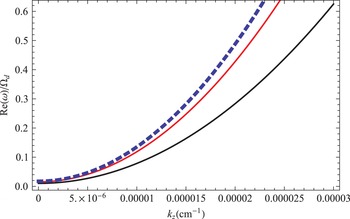
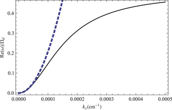
The real part of the normalized frequency (with dust gyro-frequency) are drawn as a function of $k_{z}$ for different values of spectral index ${\it\kappa}$ . These are ${\it\kappa}=2$ (the bottom solid line), for ${\it\kappa}=3$ (the middle red line) and for ${\it\kappa}=4$ (the top dashed blue line).

Figure 2.

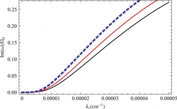
The normalized growth rate of the instability (with dust gyro-frequency) are drawn for different values of $T_{i}$ as a function of $k_{z}$ . $T_{i}=0.1T_{e}$ (the bottom solid line), $0.12T_{e}$ (the middle red line) and $0.15T_{e}$ (the top dashed blue line), keeping the spectral index ${\it\kappa}=2$ fixed.

Keeping the other parameters fixed, we plot the dispersion relation in figure 1, for ${\it\kappa}$ values of 2, 3 and 4. It is evident that when the value of the spectral index increases, where the concentration of the high energy particles decreases, the phase velocity of the waves increases. This means that the phase velocity is maximum for a Maxwellian plasma, since higher values of ${\it\kappa}$ approach the Maxwellian limit. Physically, this may be possible due to the fact that as the population of the energetic particles increases in the tail of the distribution, the width of the corresponding distribution decreases. Since the width of the distribution functions represent the kinetic temperature of the species, thus the temperature might be decreased with the kappa distribution. It also reflects that the non-thermal characteristic of the plasma particles increases. It is also possible to say that the corresponding kinetic temperature decreases or the effective temperature decreases. Thus the phase velocity of the electrostatic waves under consideration decreases in non-Maxwellian plasmas when compared to Maxwellian plasmas.

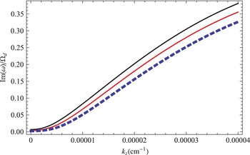
Figure 2 exhibits the result of the variation of ion temperature on the imaginary root (i.e. instability) of the mode for fixed kappa ( ${\it\kappa}=2$ ). It is evident from the plot that when the temperature of the ions increases the overall temperature $(T_{eff})$ of the system increases. This enhances the acoustic speed of the wave. Thus the instability (which is essentially due to dust charging effect) shows direct dependence on the effective temperature, which is clear from figure 2, i.e. the growth rate of the instability increases with an increase in the ion temperature. figure 3 reflects the behaviour of the instability with the electron density for fixed kappa value. In this case, the instability increases by increasing the electron number density. 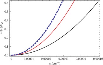Figure 4 shows the effect of the dust charge number $Z_{d0}$ on the phase velocity of the mode. It is clear that the phase velocity decreases when using greater value of the dust charge parameter. Physically, this means that as the dust charge parameter increases, the number of electrons residing on the dust particle increases while the number of freely available electrons decrease so the effective temperature decreases and correspondingly the phase velocity of the waves decrease. The dust drift mode (versus $k_{\boldsymbol{y}}$ ) is shown in figure 5, for both $c_{d}\neq 0$ and $c_{d}=0$ . 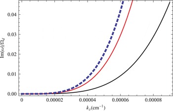This shows that, due to parallel dust dynamics, the drift wave frequency becomes a little higher. Figure 6 shows that the dust drift wave instability ( $c_{d}k_{z}\simeq 0$ ) increases with the increase in kappa.

Figure 3.

The normalized growth rate of the instability (with dust gyro-frequency) for different values of $n_{e}$ as a function of $k_{z}$ , for $n_{e}=100$ (the top solid line), $n_{e}=500$ (the middle red line) and $n_{e}=1000$ (the bottom dashed blue line), keeping the spectral index ${\it\kappa}=2$ fixed.

Figure 4.

The real part of the normalized frequency (with dust gyro-frequency) for different values of $Z_{d}$ as a function of $k_{z}$ , for $Z_{d}=1000$ (the bottom solid line), $Z_{d}=2000$ (the middle red line) and $Z_{d}=3000$ (the top dashed blue line), keeping the spectral index ${\it\kappa}=2$ fixed.

Figure 5.

The real part of the normalized frequency (with dust gyro-frequency) as a function of $k_{y}$ : for $c_{d}\neq 0$ (the bottom solid line) and $c_{d}=0$ (the top dashed blue line), keeping other parameters fixed.

Figure 6.

Normalized growth rate of the instability (with dust gyro-frequency), ((3.3),  $c_{d}=0$ ) of the mode as a function of $k_{y}$ for different values of the spectral index ${\it\kappa}$ , for ${\it\kappa}=2$ (the bottom solid line), for ${\it\kappa}=3$ (the middle red line) and for ${\it\kappa}=4$ (the top dashed blue line).

6. Summary

To summarize, we have analytically studied dust drift and dust acoustic waves in a dusty plasma with non-thermal electrons, ions and the charge fluctuating dust grains. A small amplitude perturbation scheme was used to obtain the linear dispersion relation. A numerical analysis of the dispersion relation was also carried out. It is observed that the phase velocity of the electrostatic waves under consideration decreases with the inclusion of the non-thermality effect of the electrons and ions. The phase velocity of the waves also decreases by increasing the dust charge number. The growth rate of the instability increases with the increase in ion temperature. In a nonlinear regime, vortical structures can also be excited in the system. It was seen that the presence of the non-thermality effects of the electrons and ions and the dust charge fluctuations modify the condition for the existence and boundedness of dipolar vortices. These results are relevant to space plasma environments.