Implications
Bioelectrical impedance analysis provided good estimates of some carcass compositional traits of light kids. Even in the case of some traits such as muscle and fat-free soft tissue weights, that were poorly estimated by bioelectrical impedance analysis parameters, they provided useful information when combined with other measurements. The accurate estimates of carcass composition now obtained can lead to the use of bioelectrical impedance analysis as a tool to assess parameters related to carcass value of light kids. Also, offers meat producers and processors the opportunity to have an objective non-destructive technique to attach a value schedule to carcass composition.
Introduction
The use of rapid, accurate, non-invasive and inexpensive techniques in carcass quality evaluation and grading is a commitment between producers, retailers and consumers’ preference for high-quality meat. Several techniques have been reported as valuable tools for estimation of carcass composition for pig, sheep and cattle, but little information has been reported for kid carcass composition. One of these techniques is bioelectrical impedance analysis (BIA), which has provided good predictions of leaness for pig (Swantek et al., Reference Swantek, Crenshaw, Marchello and Lukaski1992 and Reference Swantek, Marchello, Tilton and Crenshaw1999; Marchello et al., Reference Marchello and Slanger1999a; Daza et al., Reference Daza, Mateos, Ovejero and López Bote2006), sheep (Jenkins et al., Reference Jenkins, Leymaster and Turlington1988; Berg and Marchello, Reference Berg and Marchello1994; Berg et al., Reference Berg, Neary, Forrest, Thomas and Kauffman1996), cattle (Marchello and Slanger, Reference Marchello, Berg, Swantek and Tilton1992; Velazco et al., Reference Velazco, Morril and Grunewald1999; Marchello et al., Reference Marchello and Slanger1999b) and buffalo (Sarubbi et al., Reference Sarubbi, Bàculo and Balzarano2008). Other techniques such as computer tomography (e.g. Bünger et al., Reference Bünger, Macfarlane, Lambe, Conington, McLean, Moore, Glasbey and Simm2011; Scholz et al., Reference Scholz, Bünger, Kongsro, Baulain and Mitchell2015) and magnetic resonance imaging (Collewet et al., Reference Collewet, Bogner, Allen, Busk, Dobrowolski, Olsen and Davenel2005; Scholz et al., Reference Scholz, Bünger, Kongsro, Baulain and Mitchell2015) have provided even better predictions of carcass and body composition. However, their cost, the low availability of the equipment required, the time taken to collect and process the data and the degree of training required for the examiner to take the necessary measurements compromise the incorporation of such techniques into existing industrial packing systems. Essentially, BIA measures the resistance (Rs) and reactance (Xc) of a constant low-intensity alternating current with a fixed frequency as it flows through a biological mass (Swantek et al., Reference Swantek, Crenshaw, Marchello and Lukaski1992). Given that lean tissues show high conductivity, whereas fat, bone and skin show low conductivity (Mialich et al., Reference Mialich, Sicchieri and Jordao2014), it becomes possible to estimate carcass fat and fat-free soft tissue, using a technique that is simple, rapid, non-invasive, inexpensive and portable. Therefore, the objective of this study was to examine the usefulness of BIA to predict carcass composition and carcass muscle chemical composition on light kid carcasses.
Material and methods
Animals and management
The experimental population consisted of 24 kids of Serrana Jarmelista Portuguese native breed. According to the traditional production method followed in the Northeast of Portugal, these animals were reared with their mothers for 40 days. After weaning all animals were fed on natural pasture and had ad libitum access to hay and water, with commercial supplement (14% CP, 3.5% crude fat, 7% crude fibre and 9% crude ash), until slaughter. Live weight (LW) at slaughter was recorded after 12 h of fasting with free access to water. The carcasses used in this study were obtained from kids that were slaughtered using standard procedures in a commercial EU licensed abattoir.
Carcass measurements, jointing and dissection
After slaughter the empty BW (EBW) was assessed. The pelt, head and all the internal organs were removed, as well as the kidney knob and channel fat. Carcasses were refrigerated for 24 h at 4°C. Cold carcass weights (CCW) were recorded. The carcasses were split along the vertebral column and the left side was cut into eight joints as outlined by Santos et al. (Reference Santos, Silva and Azevedo2008) in: leg, chump, loin, rib, anterior rib, shoulder, breast and neck. After weighing, each cut was separated into dissectible muscle, bone, subcutaneous fat, intermuscular fat and the remainder (major blood vessels, ligaments, tendons and thick connective tissue sheets associated with some muscles). All procedures were conducted in a dissection room under controlled environment with temperature maintained at 15°C. Several carcass measurements outlined by Fisher and DeBoer (Reference Fisher and De Boer1994) were taken from all carcasses: leg length (length from the symphysis pubis to the tarsal-metatarsal joint), width between trochanters, chest depth, chest perimeter, posterior buttock perimeter, anterior buttock perimeter and carcass length (CL) (length from cranial edge of the symphysis pubis to the cranial edge of the first rib). Carcass compactness, used as a conformation indicator, was determined as the ratio between CCW and CL.
Bioelectrical impedance parameters
A single frequency bioelectrical impedance analyser built specifically for this purpose, based on a high precision impedance converter AD5933 (Analog Devices Inc., 1 Technology Way, Norwood, MA, USA) integrated circuit, was used. This system combines an on-board frequency generator (that allows an external complex impedance to be excited with a known frequency) with a 12-bit, 1 MSPS, analog-to-digital converter (ADC) – the response signal from the impedance was sampled by the on-board ADC, and a discrete Fourier transform (DFT) was processed. After the adjustment with precision resistors and capacitors, and at the frequency point of 50 kHz, the magnitude of the impedance and relative phase of the impedance is calculated by the DFT algorithm obtaining the resistance (Rs) and reactance (Xc) values. The impedance (Z) was calculated as Z=(Rs2+Xc2)0.5. Considering that the resistance of a given homogeneous conductor with a uniform cross-sectional area is proportional to its length, L, and inversely proportional to its cross-sectional area, A, Rs can be calculated as Rs=pL/A, where p is the resistivity of the conductor. Given this relationship, Swantek et al. (Reference Swantek, Crenshaw, Marchello and Lukaski1992) defined two predictors of the conductor volume as Vol1=L 2/Rs and Vol2=L 2/(Rs2+Xc2)0.5, after removing p, as this is a constant, and with L as the length between detector terminals. In the present study, similar relationships were explored, just replacing L by CL: VolA=CL2/Rs and VolB=CL2/(Rs2+Xc2)0.5. Two hypodermic needles served as electrodes. They were inserted 2 cm into the carcass, ~1 cm from the dorsal midline (avoiding contact with the spinal process) at the last cervical vertebra and at the last lumbar vertebra, and provided an attachment for the connecting clips of the BIA terminal leads. Four measurements of Rs and Xc were obtained, and the mean value was considered. All bioelectrical impedance measurements were taken in cold carcasses, which were maintained at 4°C.
Carcass muscle chemical analysis
After dissection of each joint, the muscle fraction was stored in a plastic bag at −20°C. The chemical analysis of carcass muscle followed the procedure proposed by Silva et al. (Reference Silva, Gomes, Dias-da-Silva, Gil and Azevedo2005). In brief, on the day of muscle grinding, the frozen muscle samples were cut into small pieces by an electric band saw and immediately ground in a mincer (SM 200; Retsch, Haan, Germany) with an 8-mm sieve plate. Then the mixture was ground through a 4-mm sieve plate. Short breaks were carried out during the milling process to avoid sample heating. Milled carcass muscle was homogenised in an industrial mixer (Stef, Rimini, Italy). Two random samples of ~300 g were obtained from multiple subsamples of the homogenised muscle, and placed in a sealed plastic box and stored at –20°C for later chemical analysis. The samples were analysed in duplicate for moisture, ash and CP (N×6.25) and fat according to Association of Official Analytical Chemists (1990).
Statistical analysis of results
The data obtained from each carcass were analysed by simple linear regressions to evaluate the relationships of dissectible tissues and muscle chemical composition with CCW, carcass measurements and BIA parameters. Stepwise regression was used to determine which combinations of BIA parameters, carcass measurements and CCW best predicted dissectible tissues and muscle chemical composition. The simple regression equations were evaluated by the coefficient of determination (R 2 ) and residual SD (rSD). For the multiple stepwise regressions, the best fitting was also evaluated by the rSD and the adjusted coefficient of determination (Adjusted R 2 ). The Adjusted R 2 is useful in stepwise procedure to adjust for the number of variables in the model. All statistical analysis was performed by JMP (Version7; SAS Institute Inc., Cary, NC, USA).
Results
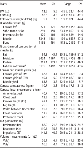
The summary data for the data collected on the experimental kids (n=24) concerning LW, carcass traits and BIA parameters, are presented in Table 1. The mean LW was 12.5 kg, but there was a large amplitude of LWs, ranging from 4.5 to 22.4 kg, which resulted in very high CV for cold carcass weight, dissectible tissues and muscle chemical composition (41.4%⩽CV⩽51.6%). Concerning carcass traits, only carcass and muscle yields showed a relatively low CV, ranging from 5.7% to 10.1%. Carcass compactness, BIA parameters and volume measurements showed quite a similar CV (respectively 31.3%, 24.7% to 31.9% and 25.6% to 26.8%), whereas CV for linear carcass measurements ranged from 12.1% to 18.2%.
Means, SD, ranges and CV for live weight (LW), empty BW (EBW), carcass traits and bioelectrical impedance analysis (BIA) parameters (n=24)

1 Carcass fat=subcutaneous plus intermuscular fat.
2 Fat-free soft tissue=protein plus moisture mass.
3 Z=(Rs2+Xc2)0.5
4 VolA=CL2/Rs.
5 VolB=CL2/(Rs2+Xc2)0.5.
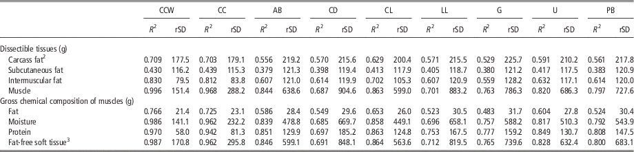
Tables 2 and 3 show the results of simple regression analysis for predicting weights of carcass dissectible tissues and muscle chemical composition with carcass measurements and with BIA and volume measurements, respectively. The amount of variation explained for each trait was quite similar for the three BIA parameters, not reaching a significant level (P>0.05) only for carcass and muscle yields (data not shown), and showing the highest accuracy in the case of dissectible carcass fat (0.814⩽R 2⩽0.862; P<0.01), which was considerably higher than the amount of variation explained by CCW, carcass compactness and carcass linear measurements for the same trait (0.529⩽R 2⩽0.709; P<0.01). For subcutaneous and intermuscular fat, the amount of variation explained by BIA parameters (respectively 0.749⩽R 2⩽0.793 and 0.718⩽R 2⩽0.760; P<0.01) was lower than for dissectible carcass fat, but still higher than the amount of variation explained by CCW, carcass compactness and carcass linear measurements for subcutaneous fat (0.379⩽R 2⩽0.439; P<0.01) and by carcass linear measurements for intermuscular fat (0.559⩽R 2⩽0.702; P<0.01). Only CCW and carcass compactness explained a larger amount of variation than BIA parameters for intermuscular fat (respectively R 2=0.830 and R 2=0.812; P<0.01). Although significant (P<0.01), the BIA parameters only explained 36.4% to 37.9% of the variation in muscle weight, whereas CCW, carcass compactness and carcass linear measurements explained 68.7% to 99.6% (P<0.01). Concerning muscle chemical composition the results for protein, moisture and fat-free soft tissue were very close to those for muscle weight, again with BIA explaining much less variation (0.344⩽R 2⩽0.393; P<0.01) than CCW, carcass compactness and carcass linear measurements (0.685⩽R 2 ⩽0.987, P<0.01). For muscle chemical fat weight the BIA parameters only explained 66.3% to 68.4% (P<0.01) of the variation observed, considerably less than the variation explained by the same measurements for dissectible carcass fat, subcutaneous fat and intermuscular fat, and also less than the variation in muscle chemical fat weight explained by CCW and carcass compactness (respectively 76.6% and 72.5%; P<0.01). The amount of variation explained by volume measurements only reached a significant level of muscle, moisture, protein and fat-free soft tissue (P<0.01 and P<0.05, respectively for VolA and VolB), even so with low accuracy, with VolA providing the best results (0.326⩽R 2⩽0.366), quite close to those of BIA parameters for the same traits.
Coefficients of determination (R 2) and residual SD (rSD) of simple regression equations for predicting weights of carcass dissectible tissues and muscle chemical composition with carcass measurementsFootnote 1

CCW=cold carcass weight; CC=carcass compactness; AB=anterior buttock perimeter; CD=chest depth; CL=carcass length; LL=leg length; G=width between trochanters; U=chest perimeter; PB=posterior buttock perimeter.
1 All coefficients of determination are significant at P<0.01.
2 Carcass fat=subcutaneous plus intermuscular fat.
3 Fat-free soft tissue=protein plus moisture mass.
Coefficients of determination (R 2) and residual SD (rSD) of simple regression equations for predicting weights of carcass dissectible tissues and muscle chemical composition with bioelectrical impedance analysis (BIA) parameters and volume measurementsFootnote 1

Rs=resistance; Xc=reactance; Z=(Rs2+Xc2)0.5; VolA=(carcass length, CL)2/Rs; VolB=(carcass length, CL)2/(Rs2+Xc2)0.5.
1 All coefficients of determination are significant at P<0.01, except those marked with * or with Ns, which are, respectively, significant at P<0.05 or not significant (P>0.05).
2 Carcass fat=subcutaneous plus intermuscular fat.
3 Fat-free soft tissue=protein plus moisture mass.
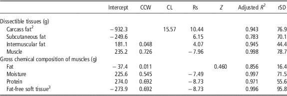
The best predictive models for carcass composition are presented in Table 4. For dissectible tissues, the best model always included one BIA measurement, namely Rs. This was even the only independent variable selected in the best model for estimation of subcutaneous fat, which was the dissectible tissue estimated with less accuracy (R 2=0.783; P<0.01). Carcass length was the only other independent variable included in the best model for estimation of carcass fat, together with Rs, explaining 94.3% of the variation observed.
Best multiple regression models for predicting weights of carcass dissectible tissues and muscle chemical composition (n=24)Footnote 1

CCW=cold carcass weight; CL=carcass length; U=chest perimeter; Rs=resistance; Xc=reactance; Z=(Rs2+Xc2)0.5.
1 All models are significant at P<0.01.
2 Carcass fat=subcutaneous plus intermuscular fat.
3 Fat-free soft tissue=protein plus moisture mass.
Discussion
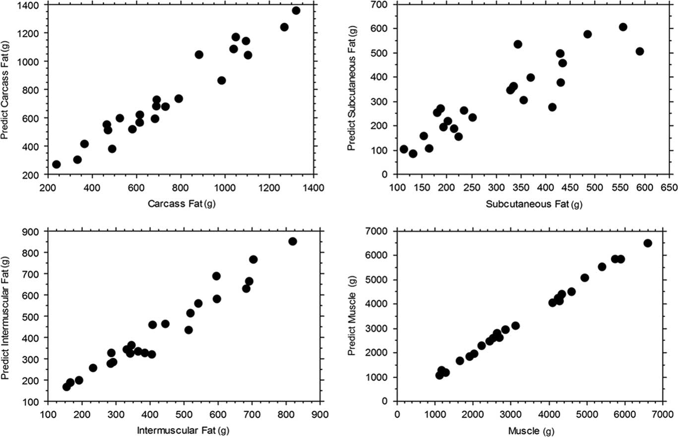
The experimental population provided data with a very large amount of variation but, despite the very high CV observed for all dissectible tissues (Table 1), which could have inflated the accuracies of the models developed, the graphs of Figure 1 show that the best prediction models obtained for carcass fat, intermuscular fat and muscle are quite robust. For subcutaneous fat, the CV observed was even higher than for the other dissectible tissues. This may be explained by the low development of subcutaneous fat in kids, already shown by Delfa et al. (Reference Delfa, Teixeira and González1994) and Teixeira et al. (Reference Teixeira, Azevedo, Delfa, Morand-Fehr and Costa1995), as small differences in absolute weight of this trait will correspond to large relative differences. With the exception of subcutaneous fat, the inclusion of Rs and just another independent variable in the prediction model resulted in a very accurate estimates (0.943⩽R 2⩽0.998; P<0.01; Table 4), with the model for prediction of muscle showing highest accuracy. Considering the low development of subcutaneous fat in kids, even the best model for prediction of subcutaneous fat, with Rs as the only independent variable, explained a large amount (78.3%; Table 4), of the variation observed.
Relationship between carcass fat, subcutaneous fat, intermuscular fat and muscle observed and predicted with the best models.

Although CCW and carcass compactness accounted, respectively, for 70.9% and 70.3% of the variation observed in carcass fat, whereas CL only accounted for 62.9% (Table 2), the inclusion of CL as the only other independent variable included in the best model for estimation of carcass fat, together with Rs, is not surprising. In fact, the variation in CL is proportional to the variation in the distance between the source and detector electrodes (L) and, as stated by Jenkins et al. (Reference Jenkins, Leymaster and Turlington1988), the value of the resistive impedance measurement is affected by L. With this in mind, several studies involving BIA parameters have included L in their best models for different species such as pigs (Swantek et al., Reference Swantek, Crenshaw, Marchello and Lukaski1992 and Reference Swantek, Marchello, Tilton and Crenshaw1999, for fat-free mass; Daza et al., Reference Daza, Mateos, Ovejero and López Bote2006, for dissected lean and fat; Marchello and Slanger, Reference Marchello, Berg, Swantek and Tilton1992, for muscle and fat-free muscle; Marchello et al., Reference Marchello and Slanger1999a, for carcass lean), lambs (Berg and Marchello, Reference Berg and Marchello1994, for fat-free mass and fat-free soft tissue; Berg et al., Reference Berg, Neary, Forrest, Thomas and Kauffman1996 and Reference Berg, Neary, Forrest, Thomas and Kauffman1997, for carcass lean and fat-free lean) and cattle (Marchello and Slanger, Reference Marchello, McLennan, Dhuyvetter and Slanger1994, for muscle and fat-free muscle; Zollinger et al., Reference Zollinger, Farrow, Lawrence and Latman2010, for percentage saleable yield and percentage of trimmable fat). Other derived variables relating Rs with CL or L have been included in combined carcass and impedance models, such as CL2/Rs and (CL2/Rs)2 (Jenkins et al., Reference Jenkins, Leymaster and Turlington1988), L 2/Rs (Vol1; Swantek et al., Reference Swantek, Crenshaw, Marchello and Lukaski1992; Velazco et al., Reference Velazco, Morril and Grunewald1999) or L 2/(Rs2+Xc2)0.5 (Vol2; Swantek et al., Reference Swantek, Crenshaw, Marchello and Lukaski1992; Velazco et al., Reference Velazco, Morril and Grunewald1999), for instance. Jenkins et al. (Reference Jenkins, Leymaster and Turlington1988) best model, for fat-free soft tissue, did include CL2/Rs and (CL2/Rs)2. More comparable with the present results, where neither VolA nor VolB were included in the best models, are the results of Swantek et al. (Reference Swantek, Crenshaw, Marchello and Lukaski1992), whose best models for fat-free mass did not include Vol1 nor Vol2. The inclusion of Rs in the best models for estimation of carcass fat and subcutaneous fat could be expected from the results of the simple regression analysis. Less expected, on the same basis, was the inclusion of Rs in the best models for estimation of intermuscular fat and muscle, as carcass compactness, for instance, explained a much larger amount of variation in these two traits than Rs. This indicates that, being CCW the independent variable that accounted for most of that variation, Rs was the independent variable that best explained the variation not accounted for by CCW. This was particularly evident for intermuscular fat, resulting in an adjusted accuracy of 94.5% for the estimates obtained with the model with CCW and Rs as independent variables, against an accuracy of 83% for the estimates based only on CCW.
Concerning muscle chemical composition, CCW was included in the best model for all traits. Despite the low accuracy of BIA parameters in the estimation of muscle chemical composition shown by simple regression analysis (Table 3), all the best models included a BIA measurement. Particularly remarkable is the effect of the inclusion of Z in the best model for muscle chemical fat weight, which resulted in an adjusted accuracy of 85.6% for the estimates obtained with the model with CCW and Z as independent variables, against an accuracy of 76.6% for the estimates based only on CCW. For muscle chemical fat weight, the results of simple regressions would already suggest the inclusion of a BIA measurement instead of any carcass linear measurement in the best model. However, the exclusion of carcass compactness from the best model for muscle chemical fat weight and of carcass compactness and carcass linear measurements from the best models for moisture, protein and fat-free soft tissue, and the inclusion in these models of a BIA parameter, indicate the higher ability of BIA to explain the variation not accounted for by CCW. As it would be expected, the coefficients for Rs concerning the estimation of muscle, moisture and protein were negative, as muscle is a highly conductive substance composed mostly of water containing electrolytes, whereas fat is an insulator that impedes the flow of an applied electrical current (Swatland, Reference Swatland1984). The best models now obtained for carcass yield of BW and EBW, and muscle yield (data not shown) included Xc and carcass measurements but, despite reaching a significant level (P<0.01) they only explained 72.1% and 75.2% respectively of the variation observed. This is consistent with the conclusion of Berg et al. (Reference Berg, Neary, Forrest, Thomas and Kauffman1996) that weights of carcass lean were more accurately predicted by BIA equations than percentages of carcass lean.
Overall, BIA parameters were useful to help predicting all the compositional traits studied, showing particular high potential in predicting carcass fat weight:
Acknowledgements
This work was supported by the Portuguese Science and Technology Foundation (FCT) under the Project PEst-OE/AGR/UID/CVT/00772/2013.