2.1 The formation mechanism of a collisionless leptonic shock

We examine the formation of shocks out of the collision of two charge- and current-neutral clouds of electrons and positrons. The plasma we consider is initially unmagnetized, no ions are present and all lepton species have the same temperature. The absent binary collisions imply that both lepton clouds will move through each other until plasma instabilities start to grow. Only three wave modes can develop for our initial conditions. The two-stream modes are purely electrostatic and their wave vector is aligned with the collision direction. The quasi-electrostatic oblique modes have a wave vector that is oriented obliquely to the collision direction and they belong to the same wave branch as the two-stream modes. The third mode is the filamentation mode, which is also known as the beam-Weibel mode (Califano et al. Reference Califano, Prandi, Pegoraro and Bulanov1998). The wave vectors of these waves form the angle $\unicode[STIX]{x03C0}/2$ with the collision direction. These three modes grow simultaneously during the shock formation stage. Their growth is eventually halted by nonlinear processes, which heat up the plasma in the overlap layer and bring it closer to a thermal equilibrium.

A leptonic shock can be created in a PIC simulation by the collision of one lepton cloud with a reflecting wall. The reflected leptons move against the inflowing leptons that have not yet reached the wall and an overlap layer develops. The instabilities in this overlap layer let waves grow that heat up the plasma when they saturate. The expansion of the heated plasma is limited on one side by the wall and a shock forms on the other side. The shock evolution is resolved correctly once a downstream region has formed that is thick enough to decouple the shock from the wall. The formation phase of the shock may, however, not be resolved correctly by this computationally efficient method. The mechanism that triggers the filamentation or beam-Weibel instability is that particles with oppositely directed current vectors repel each other and particles with parallel current vectors attract each other. The instability saturates by forming current channels that collect particles with the same direction of the current vector. Current channels that contain particles with oppositely directed current vectors are separated by magnetic fields. A reflection of a particle by the wall changes its velocity component along the wall’s normal direction and, thus, the direction of its current vector. Spatially separated current channels can, however, not form at the wall because the particle is not spatially displaced by the reflection. The suppression of the filamentation instability at the reflecting wall will affect the spectrum of the unstable waves.

This spectrum is resolved correctly if we let two separate lepton clouds collide. If both clouds differ only in their mean speed, then we have to resolve in the simulation two identical shocks that enclose the expanding downstream region. It is computationally expensive and unnecessary to track both shocks for a long time. Here we let a long and a short lepton cloud collide. We increase the time interval during which we can observe the shock between the downstream region and the long lepton cloud. The second shock moves into the opposite direction and it eventually reaches the simulation boundary. By that time, it no longer affects the evolution of the other shock.

2.2 The particle-in-cell simulation method

We model the collision of the lepton clouds with a PIC simulation. The PIC simulation code is based on the kinetic plasma model, which approximates each plasma species $i$ by a phase space density distribution $f_{i}(\boldsymbol{x},\boldsymbol{v},t)$ . The position vector $\boldsymbol{x}$ and the velocity vector $\boldsymbol{v}$ are treated as independent coordinates, which allows for arbitrary velocity distributions at any given position. The number density of this species is the zeroth moment of the distribution $n_{i}(\boldsymbol{x},t)=\int f_{i}(\boldsymbol{x},\boldsymbol{v},t)\,\text{d}\boldsymbol{v}$ and the mean speed $\bar{\boldsymbol{v}}_{i}(\boldsymbol{x},t)=\int \boldsymbol{v}f_{i}(\boldsymbol{x},\boldsymbol{v},t)\,\text{d}\boldsymbol{v}$ corresponds to its first moment. The number density and the mean speed yield the charge density $\unicode[STIX]{x1D70C}_{i}(\boldsymbol{x},t)=q_{i}n_{i}(\boldsymbol{x},t)$ and the current density $\boldsymbol{J}_{i}(\boldsymbol{x},t)=q_{i}\bar{\boldsymbol{v}}_{i}(\boldsymbol{x},t)n_{i}(\boldsymbol{x},t)$ of the species $i$ . The total charge density $\unicode[STIX]{x1D70C}(\boldsymbol{x},t)=\sum _{i}\unicode[STIX]{x1D70C}_{i}(\boldsymbol{x},t)$ and current density $\boldsymbol{J}(\boldsymbol{x},t)=\sum _{i}\boldsymbol{J}_{i}(\boldsymbol{x},t)$ update the electromagnetic fields via a finite difference approximation of Ampere’s and Faraday’s laws on a numerical grid.

The EPOCH code (Arber et al. Reference Arber, Bennett, Brady, Lawrence-Douglas, Ramsay, Sircombe, Gillies, Evans, Schmitz and Bell2015) we use fulfils $\unicode[STIX]{x1D735}\boldsymbol{\cdot }\boldsymbol{B}=0$ and $\unicode[STIX]{x1D735}\boldsymbol{\cdot }\boldsymbol{E}=\unicode[STIX]{x1D70C}/\unicode[STIX]{x1D716}_{0}$ to round-off precision.

An ensemble of computational particles (CPs) with charge $q_{i}$ and mass $m_{i}$ approximates the phase space density distribution $f_{i}(\boldsymbol{x},\boldsymbol{v},t)$ . The relativistic momentum $\boldsymbol{p}_{j}$ of the $j$ th CP of species $i$ is updated via a discretized form of the relativistic Lorentz force equation $(\unicode[STIX]{x2202}/\unicode[STIX]{x2202}t)\boldsymbol{p}_{j}=q_{i}(\boldsymbol{E}(\boldsymbol{x}_{j})+\boldsymbol{v}_{j}\times \boldsymbol{B}(\boldsymbol{x}_{j}))$ and its position is updated via $(\unicode[STIX]{x2202}/\unicode[STIX]{x2202}t)\boldsymbol{x}_{j}=\boldsymbol{v}_{j}$ . The electric field and the magnetic field are interpolated from the numerical grid to the particle’s position $\boldsymbol{x}_{j}$ to update its momentum. The current density on the grid, which is used to update the electromagnetic fields, is the sum over all particle currents after they have been interpolated from the particle positions to the grid nodes.

2.3 The simulation set-up

Our two-dimensional simulation box has the length $L_{x}$ along $x$ and $L_{y}$ along $y$ . The simulation box is subdivided into the two intervals $-0.65L_{x}<x<0$ and $0\leqslant x<0.35L_{x}$ . The boundary at $0.35L_{x}$ is reflecting and that at $-0.65L_{x}$ is open. The boundary conditions at $y=0$ and $y=L_{y}$ are periodic. We place electrons and positrons with equal densities $n_{0}$ and temperatures $T_{0}=10~\text{eV}$ everywhere in the box at $t=0$ . The electrons and positrons in the interval with $x\geqslant 0$ have a vanishing mean speed. The electrons and positrons in the interval $x<0$ have the mean speed $v_{0}=0.2c$ along $x$ . No new particles are introduced while the simulation is running and the simulation is stopped well before the end of the inflowing lepton cloud encounters the shock or before the leptons that are reflected by the boundary at $x=0.35L_{x}$ return to the shock.

We normalize the position to the electron skin depth $\unicode[STIX]{x1D706}_{s}=c/\unicode[STIX]{x1D714}_{p}$ , where $\unicode[STIX]{x1D714}_{p}=(n_{0}e^{2}/\unicode[STIX]{x1D716}_{0}m_{e})^{1/2}$ is the electron plasma frequency of one cloud. Velocities are normalized to $c$ . Momenta are normalized to $cm_{e}$ and we define $p_{0}=v_{0}m_{e}$ as the mean momentum of a lepton of the plasma cloud in the half-space $x<0$ . The box size $L_{x}\times L_{y}=60\times 2.4$ is resolved by $1.9\times 10^{4}$ grid cells along $x$ and by 760 grid cells along $y$ . Electrons and positrons are represented by 25 CPs per cell, respectively. The time is normalized to $\unicode[STIX]{x1D714}_{p}^{-1}$ . The simulation time $t_{sim}=120$ , which is subdivided into 57 200 equal time steps. We normalize the electric field to $\unicode[STIX]{x1D714}_{p}cm_{e}/e$ and the magnetic field to $\unicode[STIX]{x1D714}_{p}m_{e}/e$ .

2.4 The solution of the linear dispersion relation

We have to verify that our box is large enough to resolve the competing unstable modes and we want to determine the wave mode which grows fastest for the selected initial conditions. We solve for this purpose the linear dispersion relation in order to determine the spectrum of the growing waves. The solution is computed under the assumption that the overlap layer has an infinite size. This condition is approximately fulfilled if the colliding clouds can interpenetrate for some time before the instabilities grow.

The initial velocity spread for $T_{0}=10~\text{eV}$ is approximately $v_{th0}=4.5\times 10^{-3}c$ and both clouds drift toward each other at $v_{0}=0.2c$ . Thermal effects can be neglected for the ratio $v_{0}/v_{th0}=44$ and the lepton beams are cold. We solve the linear dispersion relation in the frame of reference in which the total momentum vanishes. The pair clouds move in this reference frame into opposite $x$ directions at the speed modulus $\unicode[STIX]{x1D6FD}_{0}^{\prime }\equiv v_{0}^{\prime }/c=1/10$ .

The non-relativistic dispersion equation for a perturbation of the form $\exp (\text{i}\boldsymbol{k}\boldsymbol{\cdot }\boldsymbol{r}-\text{i}\unicode[STIX]{x1D714}t)$ and a wave vector $\boldsymbol{k}$ with an arbitrary orientation is (Bret, Gremillet & Dieckmann Reference Bret, Gremillet and Dieckmann2010)

where $\unicode[STIX]{x1D6FF}_{\unicode[STIX]{x1D6FC}\unicode[STIX]{x1D6FD}}$ is the Kronecker symbol and

The problem of finding the fastest-growing mode has been solved (Bret & Deutsch Reference Bret and Deutsch2005; Bret et al. Reference Bret, Stockem, Fiuza, Ruyer, Gremillet, Narayan and Silva2013) for cold distributions of the form $f_{j}^{0}(\boldsymbol{p})=\unicode[STIX]{x1D6FF}(p_{y})\unicode[STIX]{x1D6FF}(p_{x}-P_{j})$ .

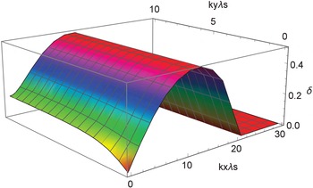
Figure 1 shows the solution of the linear dispersion relation for our plasma parameters.

Figure 1.

The solution of the linear dispersion relation for two beams, each of which consists of electrons and positrons with the same number density, mean speed and temperature $T_{0}=10~\text{eV}$ . The beams have an infinite extent and they counter-stream along $x$ with the speed modulus $0.1c$ . The growth rate $\unicode[STIX]{x1D6FF}$ is expressed in units of $\unicode[STIX]{x1D714}_{p}$ .

The growth rate peaks at the wavenumber $k_{x}\unicode[STIX]{x1D706}_{s}\approx 12$ and its value does not depend on $k_{y}\unicode[STIX]{x1D706}_{s}$ for the considered wavenumber interval. The fastest-growing modes are thus the two-stream/oblique modes. Their peak exponential growth rate is

The filamentation modes are characterized by a flow-aligned component $k_{x}=0$ . Califano et al. (Reference Califano, Prandi, Pegoraro and Bulanov1998) estimated their growth rate as

Figure 1 demonstrates that the growth rate of the filamentation modes with $k_{x}=0$ is smaller than that of the two-stream/oblique modes, which confirms the aforementioned approximations since $\unicode[STIX]{x1D6FF}_{W}<\unicode[STIX]{x1D6FF}_{TS}$ for $\unicode[STIX]{x1D6FD}_{0}^{\prime }=1/10$ .

We can estimate with the help of figure 1 if and how our limited box size will affect the spectrum of growing waves. The simulation employs periodic boundary conditions along $y$ and the box length is $L_{y}$ in this direction. The smallest resolved wavenumber is thus $k_{c}=2\unicode[STIX]{x03C0}/L_{y}$ or $k_{c}\unicode[STIX]{x1D706}_{s}=2.6$ and waves with $k_{y}<k_{c}$ cannot grow. Figure 1 shows that the growth rate of the filamentation modes decreases below $\unicode[STIX]{x1D6FF}_{W}$ for $k_{y}<k_{c}$ while that of the two-stream/oblique modes remains unchanged. The main effect of the limited box size along $L_{y}$ is thus to suppress the wavenumbers where the growth of the filamentation instability is negligible. If our simulation shows that the plasma dynamics is governed by the two-stream/oblique modes, then we would obtain the same result also for larger $L_{y}$ .

3.1 Instability and nonlinear saturation

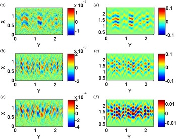
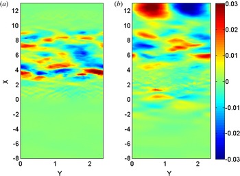
The two clouds of initially unmagnetized collisionless lepton plasma will move through each other for some time before plasma instabilities set in. Figure 2(a–c) displays the electric $E_{x}$ and $E_{y}$ components as well as the magnetic $B_{z}$ component at the time $t_{1}=7.6$ . The lepton cloud, which was initially located in the half-space $x<0$ , has moved by $v_{0}t_{1}=1.5$ towards increasing values of $x$ . Waves have grown in the cloud overlap layer, which spans the interval $0<x<1.5$ at this time. The distribution of $E_{x}$ reveals waves with a wavelength $\unicode[STIX]{x1D706}\approx 0.4$ . The $E_{y}$ and $B_{z}$ components are closely correlated and both oscillate rapidly along $y$ .

Figure 2.

The in-plane electric field and the out-of-plane magnetic field close to the initial collision boundary at the time $t_{1}=7.6$ (a–c) and at $t_{2}=14.7$ (d–f): panels (a,d) show $E_{x}$ , panels (b,e) show $E_{y}$ and panels (c,f) show $B_{z}$ .

The in-plane electric field components and the out-of-plane magnetic field at the time $t_{2}=14.7$ are displayed in figure 2(d–f). Figure 2(a,d) show the same distribution of $E_{x}$ except for the larger amplitude. Their spatial confinement demonstrates that these waves do not propagate along $y$ . The wave structures belong to electrostatic two-stream modes. The patterns in $E_{y}$ resemble those in $B_{z}$ and their amplitude ratio is comparable to that at the earlier time. The spatial correlation of the field structures in the distribution of $E_{y}$ and $B_{z}$ suggests that they belong to the same waves.

We can extract some properties of the waves from a comparison of the amplitude of $E_{y}$ and $B_{z}$ at the times $t_{1}$ or $t_{2}$ . The ratio of the field energy densities $\unicode[STIX]{x1D716}_{0}(E_{x}^{2}+E_{y}^{2})/2$ and $B_{z}^{2}/2\unicode[STIX]{x1D707}_{0}$ is in the given normalization $(E_{x}^{2}+E_{y}^{2})/B_{z}^{2}\approx 100$ . The particles of both clouds move at a speed ${\approx}v_{0}/2$ relative to the waves, which are slow moving in the reference frame of the overlap layer. The electric force imposed on a charged particle, which moves with $v_{0}/2=0.1$ , is 50 times larger than the magnetic force. We conclude that the wave’s magnetic field neither has a significant energy density nor does it affect the lepton dynamics. The waves are thus quasi-electrostatic and their wavelength along the collision direction is ${\approx}0.4$ . The amplitude of the waves has increased by a factor ${\approx}50$ during the time interval $t_{2}-t_{1}=7.1$ . If we assume that the waves grow exponentially, then their growth rate is $\unicode[STIX]{x1D6FF}\approx 0.5$ in units of $\unicode[STIX]{x1D714}_{p}$ , which matches that in figure 1.

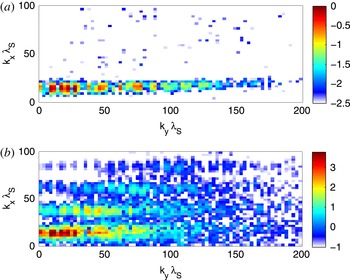
The wave modes that yield the observed electric field can be identified with its spatial power spectrum. We Fourier transform the in-plane electric field distribution $E_{p}(x,y)=E_{x}(x,y)+iE_{y}(x,y)$ over the spatial interval $0.2<x<2.7$ and over all $y$ and multiply it with its complex conjugate. Figure 3(a,b) show the power spectra at the times $t_{1}$ and $t_{2}$ in the quadrant $k_{x}>0$ and $k_{y}>0$ . The power spectrum at $t_{1}=7.6$ shows wave power at $k_{x}\unicode[STIX]{x1D706}_{s}\approx 14$ , which extends up to maximum perpendicular wavenumber $|k_{y}\unicode[STIX]{x1D706}_{s}|\approx 200$ . The wavenumber $k_{x}\unicode[STIX]{x1D706}_{s}=14$ corresponds to a wavelength along $x$ of approximately 0.45.

Figure 3.

The spatial power spectra of the in-plane electric field $E_{p}=E_{x}(x,y)+iE_{y}(x,y)$ at the time $t_{1}=7.6$ (a) and $t_{2}=14.7$ (b). The colour scale is 10-logarithmic and both spectra are normalized to the peak value in (a).

The flow-aligned wavenumber $k_{x}\unicode[STIX]{x1D706}_{s}\approx 14$ of the fastest-growing waves and the extension of wave power to large values of $k_{y}$ agree with the numerical solution of the linear dispersion relation in figure 1. The solution of the linear dispersion relation predicts a peak growth rate that does not depend on the value of $k_{y}$ for the considered wavenumbers. The wave spectrum in figure 3(a) does however suggest that waves with a low value of $k_{y}$ grow faster. The growth rate is proportional to the amplitude the wave would reach after a given time if its growth would not be limited by nonlinear effects. The electric field amplitude, which is necessary to form phase space vortices, decreases with increasing values of $k={|k_{x}^{2}+k_{y}^{2}|}^{1/2}$ (O’Neil Reference O’Neil1965) and the discrepancy between the spectral distribution in figure 3(a) and the solution of the linear dispersion relation in figure 3(c) can thus be explained with a stronger nonlinear damping that is imposed on the modes with a large value of $k_{y}$ .

The power spectrum in figure 3(b) is still concentrated on the two-stream/oblique mode branch. Its width along $k_{y}$ has diminished, which suggests that thermal damping is at work; the range of wavenumbers $k_{y}$ that are unstable to the oblique mode instability is large in a cold plasma, while the wave growth is concentrated at low values of $k_{y}$ if the plasma is hot (Silva et al. Reference Silva, Fonseca, Tonge, Mori and Dawson2002). A first and second harmonic along $k_{x}$ have emerged. The wave amplitudes have thus reached a nonlinear regime (Umeda et al. Reference Umeda, Omura, Yoon, Gaelzer and Matsumoto2003).

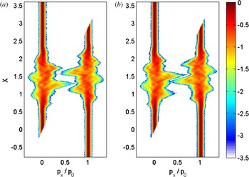
Nonlinear effects in the wave distribution should be tied to changes in the lepton distribution. Figure 4 shows the phase space density distributions $f(x,p_{x})$ of the electrons and positrons. The overlap layer of both clouds spans the interval $-0.2<x<3$ . The counter-streaming clouds have not yet merged along $p_{x}$ . However, the substantial particle acceleration demonstrates that the instability is about to saturate. The density in the overlap layer is twice that of a single cloud and the density fluctuations caused by the waves are of the order of 5 %–10 % (not shown).

Figure 4.

The phase space density distribution in the $x,p_{x}$ -plane at the time $t_{2}=14.7$ of electrons (a) and positrons (b). The phase space density distribution is averaged over all other dimensions. The momentum is normalized to $p_{0}$ . The colour scale is 10-logarithmic.

The filamentation instability starts to grow immediately but the two-stream instability outgrows it.

3.2 Shock formation

The two-stream instability saturates by forming stable phase space vortices in the electron and positron distributions (Berk & Roberts Reference Berk and Roberts1967) and the same holds during the initial saturation stage of the oblique mode instability (Dieckmann et al. Reference Dieckmann, Frederiksen, Bret and Shukla2006b ). Electron phase space vortices are characterized by strong bipolar pulses in the electric field distribution, which correspond to a localized positive excess charge. Positron phase space vortices correspond to a localized negative excess charge.

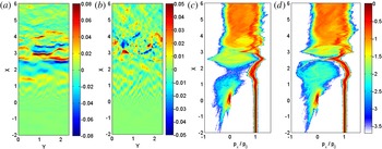
The in-plane electric field components at the time $t_{3}=58.8$ are displayed in figure 5(a,b). The $E_{x}$ component is animated in time in panel (a) of Movie 5(a,b), in the supplementary materials while panel (b) shows the time evolution of the $E_{y}$ component. The electric $E_{x}$ component shows such bipolar field structures. A large quasi-planar field pulse is located at $x\approx 2.5$ in the interval starting from $y\approx 1$ that goes through the periodic boundary at $y=2.4$ until $y\approx 0.5$ . The polarity of $E_{x}$ indicates the presence of a positive excess charge in between both electric field bands. If this quasi-planar bipolar pulse is associated with an electron phase space vortex, then the latter should be detectable in the electron phase space density distribution even if it has been integrated over all values of $y$ .

Figure 5.

Panels (a) and (b) show the electric $E_{x}$ and $E_{y}$ components close to the initial collision boundary. Panels (c) and (d) show the phase space density distributions in the $x,p_{x}$ -plane of electrons and positrons, respectively. The phase space density distributions are averaged over all other dimensions, they are normalized to the same value and displayed on a 10-logarithmic scale. The momentum is normalized to $p_{0}$ . The simulation time is $t_{3}=58.8$ .

Figure 5(c,d) show the corresponding electron and positron distributions. The time-evolution of the electron phase space density distribution is shown in panel (c) of Movie 5(c,d) in the supplementary materials while panel (d) shows that of the positrons. Figure 5(c) confirms the existence of a phase space vortex in the electron distribution at this location. The vortex in figure 5(c) spans the spatial interval $2<x<3$ and the momentum interval $-1<p_{x}/p_{0}<1$ . The mean momenta of the upstream electrons and positrons are modulated by the electrostatic potential of the vortex when they pass it, but they are not trapped by it. The upstream leptons continue to move to increasing values of $x$ until they are thermalized upon entering the downstream region $x>4$ , which is characterized by a dense phase space density distribution between $0<p_{x}/p_{0}<1$ . This thermalization can only be accomplished by the field structures seen in the in-plane electric field between $x\approx 3$ and $x\approx 4$ in figure 5(a,b).

The distribution of the positrons shows two smaller vortices that surround the large electron phase space vortex. The positron vertices are centred at $x\approx 1.8$ and $x\approx 3$ . The zero crossing of the electric $E_{x}$ component and, thus, the extremal point of the electrostatic potential at $x\approx 2.5$ in figure 5(a) corresponds to a stable equilibrium point for the trapped electrons. Hence it is an unstable equilibrium point for the positrons, explaining why the vortices of positrons and electrons are staggered along $x$ .

A small localized cloud of electrons and positrons is centred at $x\approx 0$ and $p_{x}\approx 0$ . The cloud is an artefact from our initial conditions. The finite growth time of the electrostatic instabilities implies that the waves start to grow well behind the front of the plasma cloud that was initially located in the half-space $x>0$ . This charge- and current-neutral cloud is stable against electrostatic instabilities because its extent along $x$ is not sufficiently large to allow it to interact with the inflowing upstream leptons via a two-stream instability.

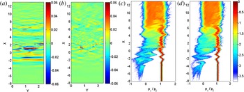
Figure 6 shows the in-plane electric field distribution and the associated lepton phase space density distributions at the time $t_{4}=120$ . We observe strong quasi-planar electric field structures in the $E_{x}$ -distribution in the interval $-3<x<0$ . Their amplitude is comparable to the one that gave rise to phase space vortices in the electron and positron distributions at the earlier time. These electrostatic structures in $E_{x}$ have propagated well beyond the initial collision boundary $x=0$ reaching a position $x\approx -3$ . We find relatively strong electric field oscillations in $E_{x}$ and $E_{y}$ between $0<x<8$ . The transition layer of this shock thus spans at this time an interval with the width $\unicode[STIX]{x0394}x\approx 10$ .

Figure 6.

Panels (a) and (b) show the electric $E_{x}$ and $E_{y}$ components close to the initial collision boundary. Panels (c) and (d) show the phase space density distributions in the $x,p_{x}$ -plane of electrons and positrons, respectively. The phase space density distributions are averaged over all other dimensions, they are normalized to the same value and displayed on a 10-logarithmic scale. The momentum is normalized to $p_{0}$ . The simulation time is $t_{4}=120$ .

The strong planar waves in the interval $-3<x<0$ in figure 6 are correlated with phase space vortices in the hot lepton population at low speeds. The vortices of electrons and positrons are staggered along $x$ . The electrons and positrons that gyrate in these vortices originate from the hot plasma component and they are well separated along $p_{x}$ from the inflowing upstream leptons. The mean speed of these phase space vortices is less than $p_{x}=0$ , which implies that they move towards decreasing values of $x$ . The mean speed of the vortices decreases with an increasing distance from the shock transition layer and they are thus accelerated away from the downstream plasma. The leptons, which gyrate in the vortices, reach a peak momentum ${\approx}-p_{0}$ .

The simultaneous presence in the interval $-6<x<5$ of the hot leptons that have leaked from the downstream region and the cooler drifting upstream leptons implies that the overall plasma distribution is non-thermal and thus unstable. The electric field of the phase space vortices seeds the instability and we observe momentum oscillations along $p_{x}$ in the cool inflowing electrons and positrons that increase with $x$ in the interval $-3<x<-1$ . The oppositely directed oscillations of electrons and positrons result in a strong current, which induces an electric field. The electric field oscillates in space and its oscillation amplitude decreases in unison with the net current in the direction of decreasing values of $x$ . We can describe this oscillation in terms of a product between a sinusoidally oscillating electric field and an envelope function.

Figure 7.

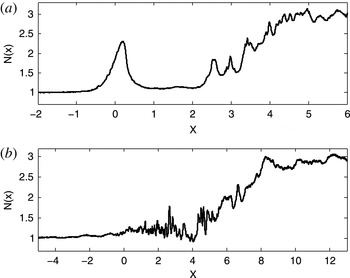
The total lepton density $N(x)$ in units of the initial total density $2n_{0}$ at the time $t_{3}=58.8$ (a) and $t_{4}=120$ (b).

A spatially varying envelope function gives rise to a ponderomotive force (Kono, Skoric & ter Haar Reference Kono, Skoric and ter Haar1980) that does not depend on the sign of the particle charge and accelerates electrons and positrons in the direction of decreasing values of the envelope function. This ponderomotive force is exerted by the modulated upstream plasma onto the hot leptons that form the phase space vortices and it accelerates them.

The leptons in the interval $1<x<6$ in figure 6(c,d) are composed of a hot dilute component and the cool dense upstream leptons. Both populations gradually mix and they merge to a single one at $x\approx 6$ . We observe electric fields in this interval in figure 6. These fields show some piecewise planar structures, which correspond to phase space vortices with a limited extent along $y$ . The two strongest localized structures at $x\approx 1$ are separated by a perpendicular $E_{y}$ field at $y\approx 0.8$ . These localized structures are likely to be the result of an instability of initially planar phase space vortices or phase space tubes. Indeed, two-dimensional PIC simulations (Oppenheim, Newman & Goldman Reference Oppenheim, Newman and Goldman1999) of phase space tubes in a stabilizing magnetic field show that the phase space tubes gradually break up along their axes. The collapse of a phase space vortex is an effective way to scatter the leptons in phase space, which results in a mixing of the downstream and upstream leptons in the $x,p_{x}$ plane. Strong small-scale electric fields are observed up to $x\approx 8$ . The absence of phase space vortices with $x>8$ demonstrates that the lepton distribution in this interval is no longer unstable to electrostatic instabilities.

The phase space density distribution of the leptons was uniform in the interval $4<x<6$ at the time $t_{3}=144$ and in the interval $7<x<13$ at the time $t_{4}=297$ . We conclude that these intervals correspond to a downstream region that is close to being in a thermal equilibrium, at least with respect to electrostatic waves and instabilities. The density distribution along $x$ sheds light onto how much the plasma is compressed by the shock crossing. Figure 7 compares the density distributions at the times $t_{3}$ and $t_{4}$ . The density converges at low $x$ to the initial density. A density peak is observed close to $x\approx 0$ in figure 7(a), which corresponds to the dense lepton cloud at this position shown in figure 5(a). The density peak has disappeared in figure 7(b). The electric fields that grew in this spatial interval in response to the instability between the inflowing upstream leptons and the leaked hot downstream leptons tore the cloud apart by accelerating the electrons and positrons into opposite directions. The density rises from approximately $N(x)=1$ to $N(x)\approx 3$ over a few electron skin depths. The plasma compression factor of approximately 3 is the one expected for a strong non-relativistic shock (Zel’Dovich et al. Reference Zel’Dovich, Raizer, Probstein and Hayes1967).

3.3 Secondary instabilities and magnetic field generation

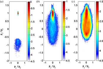
The electric fields associated with the phase space vortices heat up the leptons via Landau damping (Landau Reference Landau1946; O’Neil Reference O’Neil1965) and their collapse scatters them in phase space. The effects of this heating on the lepton distribution is visualized by figure 8, which shows the phase space density as a function of $p_{x}$ and $p_{y}$ at three positions along $x$ . The distribution has been integrated over $y$ and over an interval along $x$ of width 0.3.

Figure 8.

The total lepton distribution $f_{t}(v_{x},v_{y})$ averaged over $-4.5<x<-4.2$ is shown in panel (a), that averaged over $1.9<x<2.2$ in panel (b) and that averaged over $8.3<x<8.6$ is shown in panel (c). The colour scale is 10-logaritmic and normalized to the peak value in (a).

The distribution in figure 8(a) has been sampled far upstream of the shock. The upstream leptons constitute the cold dense beam that is located at $p_{x}\approx p_{0}$ . The leaked leptons form a hot and dilute beam that moves at $p_{x}\approx -p_{0}$ . The mean speed of the hot lepton beam exceeds that expected from a specular reflection, since the shock is moving to increasing values of $x$ . Figure 8(b) reveals that the inflowing upstream leptons have been heated up by the time they reach the position $x\approx 2$ . They are distributed over a wider velocity range and their peak value of the phase space density has thus decreased. The temperature is of the order of 100 eV. These leptons are immersed in a hot dilute lepton component. Its thermal momentum spread is of the order of $p_{0}$ and the temperature is thus approximately one keV. The inflowing upstream leptons form a hot beam at $p_{x}\approx p_{0}$ in figure 8(c) that is only approximately twice as dense as the leptons in the hot population.

The waves observed close to $x=2$ in figure 6(a,b) suggest that the velocity distribution in figure 8(b) is still unstable to an electrostatic instability. It cannot be the two-stream instability because that one requires two beams that are well separated along $p_{x}$ . This distribution can, however, still be unstable to the electron acoustic instability. Like the well-known ion acoustic instability, which is driven by a drift between cold ions and hot electrons, the electron acoustic instability can develop if cold electrons drift relative to a hot electron species. Waves grow if the drift speed between the hot and the cold electron species exceeds several times the thermal spread of the cold electron species (Gary Reference Gary1987). This condition is fulfilled in figure 8(b). We note in this context that although the phase space density of the hot leptons is two orders of magnitude less than that of the inflowing upstream leptons, their number density, which we obtain by integrating the phase space density along $p_{x}$ , is of the same order. The interaction of counter-streaming lepton beams with a similar density results in rapidly growing instabilities. To the best of our knowledge the acoustic instability in pair plasma has not yet been explored. Here we cannot unambiguously show that it exists in pair plasma, because the electric field may also be the residual field of a phase space hole that formed previously.

The distribution in figure 8(c) appears to be stable against electrostatic instabilities since we do not observe significant electric field oscillations in the region $x>8$ . The velocity distribution of the leptons in this region is, however, not a Maxwellian. Therefore the plasma contains free energy that can be released by a collisionless instability. The thermal anisotropy contained in the total lepton velocity distribution $f_{t}(v_{x},v_{y})$ and measured in the rest frame of the downstream plasma can be estimated as

A value $A=0$ would say that the thermal energy in the $x$ direction equals that in the $y$ direction, which would imply that there is no thermal anisotropy. We obtain the value $A\approx 6$ from the data shown in figure 8(c). Such a large anisotropy value results in the Weibel instability in its original form (Weibel Reference Weibel1959; Morse & Nielson Reference Morse and Nielson1969).

Figure 9 confirms that a magnetic field has grown in the downstream region. Movie 9 in the supplementary materials animates the evolution of the magnetic $B_{z}$ component in time. Strong magnetic fields with approximately the same peak amplitude are present at both times. The amplitude of the magnetic field exceeds that observed in figure 2(c,f) by a factor 3 and it equals that of the electric field in the given normalization in figure 6(a,b). Nevertheless, the magnetic force, which is acting on a lepton that is moving at the speed of 0.1 relative to these field patches, will still be an order of magnitude weaker than the electric force in the shock transition layer.

Figure 9.

Panels (a) and (b) show the out-of-plane component $B_{z}$ of the magnetic field at the times $t_{3}=58.8$ and $t_{4}=120$ , respectively. The colour scale is the same for both panels. For comparison: the downstream region at $t_{3}=58.8$ is enclosed by shocks at $x\approx 3$ and $x\approx 8$ , while the correctly resolved shock at $t_{4}=120$ is located at $x\approx 5$ .

The strong downstream magnetic fields are not correlated with electric field structures (see figures 5 a,b and 6 a,b) and they are thus not driven by an oblique mode instability. The Weibel instability drives magnetowaves with a negligible electric field and with the same magnetic field direction as the one observed here and this instability is thus compatible with the simulation data. The Weibel instability yields magnetic fields with an energy density that can reach up to 10 % of the thermal energy for strong temperature anisotropies (Morse & Nielson Reference Morse and Nielson1971; Stockem, Dieckmann & Schlickeiser Reference Stockem, Dieckmann and Schlickeiser2009). The velocity spread in figure 8(c) corresponds to a lepton temperature of the order of 1 keV or $10^{7}~\text{K}$ . The magnetic pressure of a field $B_{z}=0.03$ is thus a few per cent of the cumulative thermal pressure of electrons and positrons and within the range that is accessible to the Weibel instability.

We can compare the maximum size of the magnetic patches in figure 9 to the gyroradius of an electron in that field. The magnetic field $\tilde{B}_{z}$ and the collision speed $\tilde{v}_{0}$ in physical units can be calculated from the normalized ones via $B_{z}=e\tilde{B}_{z}/m_{e}\unicode[STIX]{x1D714}_{p}$ and $\tilde{v}_{0}=v_{0}c$ . The gyroradius of an electron that moves at the speed $v_{0}/2$ relative to the stationary perpendicular magnetic field, which is normalized to $\unicode[STIX]{x1D706}_{s}=c/\unicode[STIX]{x1D714}_{p}$ , is then $r_{g}/\unicode[STIX]{x1D706}_{s}=v_{0}/2B_{z}$ . Taking $v_{0}=0.2$ and $B_{z}=0.03$ gives $r_{g}\approx 3\unicode[STIX]{x1D706}_{s}$ , which is approximately three times the coherence scale of the largest magnetic field patches. The magnetic field patches are also not stationary on the time scale needed to perform a gyro-orbit. This time equals for a maximum amplitude $B_{max}=0.03$ in our normalization $2\unicode[STIX]{x03C0}/B_{max}\approx 200$ , which exceeds the simulation time. The leptons can thus not complete a full gyro-orbit. The magnetic field will instead deflect leptons by a small angle that depends on where the lepton entered the patch and on how long it stayed inside the patch. The magnetic field will thus scatter the leptons of the directed beam in figure 8(c). The repeated scattering of the leptons will eventually thermalize their distribution.