






1. Introduction
The Fermi–Pasta–Ulam–Tsingou (FPUT) chain is a model introduced in the 1950s to study the thermal equipartition in crystals [Reference Fermi11–Reference Fermi, Pasta, Ulam and Tsingou13]. The model considers a chain of masses connected by springs with quadratic or cubic non-linearities (so-called  $\alpha$-FPUT or
 $\beta$-FPUT respectively) in their restoring forces. Fermi expected the system to reach thermalization state (e.g., with equipartition of energy in all degrees of freedom) in a short time of evolution. However, when simulated on the computer MANIAC-I, an unexpected recurrence was discovered, that the system returns to almost the exact initial condition (with energy only in large scales) after certain time of integration. Further interest and study in FPUT system led to the development of integrable theory, Korteweg–de Vries (KdV) solitons and Hamiltonian chaos [Reference Gardner, Greene, Kruskal and Miura15, Reference Schneider and Wayne24, Reference Zabusky and Kruskal29]. To some extent, the FPUT recurrence is explained by the near-integrable property of the model, but the model was later found to indeed reach thermalization over a much longer time scale [Reference Onorato, Vozella, Proment and Lvov21, Reference Ponno, Christodoulidi, Skokos and Flach23], which required further analysis.
One important development to understand the thermalization of FPUT system was via the wave turbulence (WT) theory [Reference Lukkarinen and Spohn19, Reference Onorato, Vozella, Proment and Lvov21, Reference Spohn25]. In [Reference Onorato, Vozella, Proment and Lvov21], it was shown that the WT prediction of the  $\alpha$-FPUT thermalization time scale agrees with their simulation results. The WT method was then further extended to study thermalization in
 $\beta$-FPUT and discrete non-linear Klein–Gordon models [Reference Pistone, Chibbaro, Bustamante, L’vov and Onorato22], again with agreement to simulations. The centerpiece of the WT-based argument is the derivation of a wave kinetic equation (WKE) that describes the evolution of the so-called wave action spectrum, whose evolution time scale provides the thermalization time scale. For a recent comprehensive review of the kinetic theory of oscillator chains, covering both the derivation of the WKE and the rigorous mathematical results, we refer to [Reference Germain, La and Menegaki16].
An important procedure in deriving WKE for these systems is a normal form transformation, which is a near-identity transformation enabling one to remove non-resonant terms in the dynamical equation [Reference Arnol’d1, Reference Zakharov, L’vov and Falkovich32]. Roughly speaking, these transformations are mathematically possible because the frequency condition for non-resonant interactions cannot be satisfied, so the zero-divisor problem can be avoided. However, a non-vanishing divisor does not mean that the transformation remains bounded or near-identity, and this necessary property is usually not checked in many physics literature where a normal form transformation is applied. Physically, ignoring this validity condition has important consequences, since violation of the condition corresponds to the case of quasi-resonant interactions to be associated with significant energy transfer (when the non-vanishing divisor becomes small enough). Such interactions should not be removed in this case, which otherwise leads to deviation from the true dynamics.
Clearly, the application of normal form transformation should be accompanied by a validity condition in FPUT and other Hamiltonian systems [Reference Bambusi and Ponno2, Reference Janssen17, Reference Krasitskii18, Reference Pistone, Chibbaro, Bustamante, L’vov and Onorato22, Reference Zakharov, Musher and Rubenchik31]. To the authors’ knowledge, at least two works have been carried out in this direction. The first one is [Reference Ganapa14], which attempts to establish a validity condition for the normal form transformation to remove quadratic terms in the  $\alpha$-FPUT system. However, the analysis is based on an oversimplified system only containing a few modes. Their conclusion therefore cannot be generalized to cases with a broadband spectrum (e.g., the thermal equilibrium state). The second work is [Reference Zakharov30], which deals with normal form transformation in water waves of finite depth. The analysis is done for a broadband spectrum, but random phases of modes are not considered. Because of this treatment, significant cancellations in the estimation are ignored and the final result is not consistent with the most general setting of random waves.
In this paper, we establish a validity condition of the normal form transformation in a rigorous manner. Our analysis is conducted for the  $\beta$-FPUT system to remove the four-wave non-resonant interactions, but the developed approach can be widely applied to other scenarios of Hamiltonian systems. Our analysis is carried out under the hypothesis of a random wave field: the modes are assumed to carry deterministic amplitudes of
 $O(1)$ (corresponding to a broadband spectrum close to the equipartition of wave action) and independent, identically distributed random phases, so that the validity of the transformation is understood in a statistical sense, i.e., as holding with dominant probability. We prove rigorously that, for the above-mentioned normal form transformation to stay near-identity under this hypothesis, it is required that
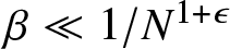
 $\beta \ll 1/N^{1+\epsilon}$, with
 $N$ the number of masses and
 $\epsilon$ an arbitrarily small constant. This result suggests physically that the relative importance of non-resonant interactions to the dynamics is governed by the parameter
 $\beta N$ (with
 $\epsilon$ omitted). We numerically confirm this point by directly computing the fraction of non-resonant terms in the Hamiltonian of a
 $\beta$-FPUT system evolving from two initial conditions, one at thermal equilibrium and the other out-of-equilibrium. For both cases, we find the fraction depends only on
 $\beta N$ as suggested by the theory.
2. Review of normal form for  $\beta$-FPUT model

We first briefly review the formulation of the  $\beta$-FPUT model and its associated normal form transformation following [Reference Bustamante, Hutchinson, Lvov and Onorato3]. The
 $\beta$-FPUT model consists of
 $N$ identical masses
 $m$ connected by non-linear springs with the elastic force
 $F=-\kappa\Delta q+\beta\Delta q^3$, where
 $\kappa,\beta\neq 0$ are spring elastic constants. The equation of motion for a
 $\beta$-FPUT chain can be expressed as (e.g., [Reference Bustamante, Hutchinson, Lvov and Onorato3, Reference Fermi, Pasta, Ulam and Tsingou13]):
 \begin{equation}
m\ddot{q}_j=\kappa\left[(q_{j+1}-q_j)-(q_j-q_{j-1})\right]+\beta\left[(q_{j+1}-q_j)^3-(q_j-q_{j-1})^3\right],
\end{equation}
where  $j=0,1,...,N-1$ and
 $q_j(t)$ represents the displacement from the equilibrium position of the mass
 $j$ with periodic boundary conditions
 $q_0=q_N$.
We consider a discrete Fourier transform
 \begin{equation}
Q_k=\frac{1}{N}\sum_{j=0}^{N-1}q_je^{-i2\pi k_j/N},\mbox{ }P_k=\frac{1}{N}\sum_{j=0}^{N-1}p_je^{-i2\pi k_j/N},
\end{equation}
with  $p_j=m\dot{q}_j$ and introduce the normal modes
 $a_k(t)$ as
 \begin{equation}
a_k=\frac{\sqrt{2}}{2}\left[(m\omega_k)^{\frac{1}{2}}Q_k+i(m\omega_k)^{-\frac{1}{2}}P_k\right], \mbox{ for }k=1,...,N-1.
\end{equation}
The evolution equation (2.1) then becomes
 \begin{align}
i\dot{a}_{k_1}=&\omega_{k_1}{a}_{k_1}+\frac{\beta}{3}\sum_{k_2,k_3,k_4}\bigg[T_{1,2,3,4}a_{k_2}a_{k_3}a_{k_4}\delta(k_1-k_2-k_3-k_4)\\ notag
&+3T_{1,-2,3,4}a_{k_2}^*a_{k_3}a_{k_4}\delta(k_1+k_2-k_3-k_4)+3T_{1,-2,3,4}a_{k_2}a_{k_3}^*a_{k_4}^*\delta(k_1-k_2+k_3+k_4)\\ notag
&+T_{1,2,3,4}a_{k_2}^*a_{k_3}^*a_{k_4}^*\delta(k_1+k_2+k_3+k_4)\bigg],
\end{align}
where the frequency and interaction coefficients read
 \begin{equation}
\omega_{k}=\omega(k)=2\sqrt{\frac{\kappa}{m}}\left|\sin\left(\frac{\pi k}{N}\right)\right|,
\end{equation}
 \begin{equation}
T_{1,2,3,4}=- \frac{3}{4\kappa^2}\iota( k_2+k_3+k_4)\iota(k_2)\iota(k_3)\iota(k_4) \prod_{i=1}^4 \sqrt{\omega_{k_i}},
\end{equation}
with  $\iota(x):=\text{sgn} \sin \left(\frac{\pi x}{N}\right)$ a
 $2N$-periodic function.
 $\delta(\cdot)$ denotes the Kronecker delta with mod
 $N$ applied to its argument. Hereafter the mod
 $N$ condition is applied to all wavenumber conditions but sometimes not written explicitly for simplicity.
Among the four terms in (2.4), only the second one with  $\delta(k_1+k_2-k_3-k_4)$ leads to resonant interactions. For the other three non-resonant terms, the corresponding frequency condition cannot be satisfied due to the positivity and strict subadditivity of
 $\omega(k)$, as well explained in [Reference Bustamante, Hutchinson, Lvov and Onorato3]. Therefore, we can remove these non-resonant terms at the current order via a normal form transformation written as
 \begin{align}
a_{k_1} =& b_{k_1}+\frac{\beta}{3}\sum_{k_2,k_3,k_4}\bigg[A^{(1)}_{1,2,3,4}b_{k_2}b_{k_3}b_{k_4}\delta(k_1-k_2-k_3-k_4)\\ notag
&+3A^{(2)}_{1,2,3,4}b_{k_2}b_{k_3}^*b_{k_4}^*\delta(k_1-k_2+k_3+k_4)
+A^{(3)}_{1,2,3,4}b_{k_2}^*b_{k_3}^*b_{k_4}^*\delta(k_1+k_2+k_3+k_4)\bigg].\end{align}
The goal here is that when (2.7) is substituted into (2.4), the resulting equation becomes
 \begin{equation}i{\dot b}_{k_1}=\omega_{k_1}b_{k_1}+\beta\sum_{k_1+k_2-k_3-k_4=0}T_{1,-2,3,4}b_{k_2}^\ast b_{k_3}b_{k_4}+O\left(\beta^2\right).\end{equation}
In order for (2.8) to be achieved, one needs to choose the coefficients of  $A^{(i)}_{1,2,3,4}$ accordingly as
 \begin{equation}
A^{(1)}_{1,2,3,4}=-\frac{T_{1,2,3,4}}{\omega_{k_1}-\omega_{k_2}-\omega_{k_3}-\omega_{k_4}},
\end{equation}
 \begin{equation}
A^{(2)}_{1,2,3,4}=-\frac{T_{1,-2,3,4}}{\omega_{k_1}-\omega_{k_2}+\omega_{k_3}+\omega_{k_4}},
\end{equation}
 \begin{equation}
A^{(3)}_{1,2,3,4}=-\frac{T_{1,2,3,4}}{\omega_{k_1}+\omega_{k_2}+\omega_{k_3}+\omega_{k_4}}.
\end{equation}
3. Validity condition of the normal form transformation
In order for the normal form transformation (2.7) to stay bounded and near-identity, we need
 \begin{equation}
\frac{\beta}{3}\left|\sum_{k_2,k_3,k_4}A^{(1)}_{1,2,3,4}b_{k_2}b_{k_3}b_{k_4}\delta(k_1-k_2-k_3-k_4)\right| \ll \left|b_{k_1}\right|
\end{equation}
and similar conditions for other sums involving  $A^{(2)}_{1,2,3,4}$ and
 $A^{(3)}_{1,2,3,4}$. A numerical study for similar conditions has been presented in [Reference Comito, Lotriglia and Bustamante4]. In addition, such a validity condition has also been formulated in [Reference Zakharov30] for gravity waves in finite water depth. However, in further estimating the sums in the LHS of the condition, the random phases in
 $b_k$ are not considered in [Reference Zakharov30], leading to an overestimation.
In order to account for the random phases in  $b_k$, we consider a field with
 $b_k=\sqrt{\phi_k}\eta_k(\varrho)$, where
 $\phi_k$’s are deterministic amplitude of
 $O(1)$ and
 $\eta_k(\varrho)$’s are i.i.d. zero-mean complex random variables with unit variance, either as standard complex Gaussian or uniformly distributed on the unit circle. Under this condition, the sum in (3.1) behaves like a random walk in a complex plane, for which cancellations due to walks in different directions must be considered. Intuitively, this sum should be evaluated as the expected value
 $\mathbb{E}[|\sum \boldsymbol \cdot|]$ or
 $\{\mathbb{E}[|\sum \boldsymbol \cdot|^2] \}^{1/2}$. Mathematically, this reasoning is guaranteed by the standard hyper-contractivity estimates as in [Reference Deng and Hani6, Lemma 3.1], which asserts that the probability of the sum
 \begin{equation}
\mathbb{P}\left(\left|\sum_{k_1-k_2-k_3-k_4=0}A^{(1)}_{1,2,3,4}b_{k_2}b_{k_3}b_{k_4}\right|\geq AM^{\frac{1}{2}}\right) \leq Ce^{-cA^{\frac{2}{3}}},
\end{equation}
for some positive constants  $A,C,c \gt 0$, with
 \begin{equation}
M=\mathbb{E}\left|\sum_{k_1-k_2-k_3-k_4=0}A^{(1)}_{1,2,3,4}b_{k_2}b_{k_3}b_{k_4}\right|^2.
\end{equation}
This hyper-contractivity lemma simply states that with dominant probability, the sum in (3.1) is estimated by  $M^{1/2}$.
By further applying the Wick contraction theorem (see [Reference Nazarenko20, Theorem 5.1]), we obtain
 \begin{equation}
M = \sum_{k_1-k_2-k_3-k_4=0}\left|A^{(1)}_{1,2,3,4}\right|^2\phi_2\phi_3\phi_4.
\end{equation}
The above calculation relies on the statistical independence of the modes. While this is assumed for the initial data, the persistence of such decorrelation, to leading order, under the non-linear flow is a non-trivial property known as propagation of chaos. As shown by Deng and Hani [Reference Deng and Hani10], for the non-linear Schrödinger (NLS) equation, the Wick contraction rules can be thought of as being preserved to leading order, in the kinetic limit (in our setting  $N\to \infty$,
 $\beta\to 0$). More precisely, there holds that any moments of the flow of the form
 \begin{equation}
\mathbb E \; b_{k_1} b_{k_2}\ldots b_{k_q}\overline{b_{\ell_1}}\, \overline{b_{\ell_2}}\ldots \overline{b_{\ell_r}} \to 0\end{equation}
in the kinetic limit, unless  $\{k_1, \ldots, k_q\}=\{\ell_1, \ldots, \ell_r\}$. While the proof in [Reference Deng and Hani10] is done for the NLS equation, it is shown to be a consequence of the same diagrammatic analysis that is used to derive the WKE. It is shown that interactions that do not respect (3.5) are vanishing in the limit, and the leading order interactions, which appear in the kinetic limit, respect (3.5). This is yet another indication of two important facts: (a) Propagation of chaos is a rather deep property that cannot be simply explained by the linear theory; it is a deep non-linear effect; (b) propagation of chaos is a fundamental constituent of the kinetic theory, and that one should not expect the latter to hold without the former. As such, propagation of chaos will hold in much wider generality, namely for any system where the kinetic theory holds, in particular for the
 $\beta$-FPUT system considered here, for which the WKE has been rigorously derived [Reference Vassilev and Wu26, Reference Wu27]. This is the foundation for the scaling
 $M^{1/2}$ used here.
Finally, we caution that while the propagation of chaos property is sometimes referred to as preservation of the random phase property, phase randomness is not really preserved at the level of the dynamics of the microscopic system but is only valid as a limiting statement (i.e., the left hand side of (3.5) is not zero at positive times, but its limit is zero).
In the Appendix A of the paper, we prove the following theorem.
Theorem 3.1. Let  $A^{(i)}_{1,2,3,4}$,
 $i=1,2,3$, be defined as in (2.9),(2.10) and (2.11), then for fixed
 $k_1 \in \mathbb{Z} \cap (0,N)$, we have:
 \begin{aligned}&\sum_{\substack{
k_1-k_2-k_3-k_4\equiv 0 \pmod N\\
k_2,k_3,k_4\in\mathbb{Z}\cap(0,N)
}}\left|A_{1,2,3,4}^{(1)}\right|^2
+\sum_{\substack{
k_1-k_2+k_3+k_4\equiv 0 \pmod N\\
k_2,k_3,k_4\in\mathbb{Z}\cap(0,N)
}}\left|A_{1,2,3,4}^{(2)}\right|^2 \\[6pt]
&\quad +\sum_{\substack{
k_1+k_2+k_3+k_4\equiv 0 \pmod N\\
k_2,k_3,k_4\in\mathbb{Z}\cap(0,N)}}
\left|A_{1,2,3,4}^{(3)}\right|^2
\lesssim N^2\log N.
\end{aligned}
Combining (3.1) (and the counterparts for other sums), (3.4) and Theorem 3.1, we conclude that the validity condition of the normal form transformation is
 \begin{equation}
\beta \ll \frac{1}{N^{1+\epsilon}},
\end{equation}
where  $\epsilon$ is an arbitrarily small constant, resulting from the
 $\log N$ factor in (3.6) for large
 $N$. We remark that the sharp condition following from (3.1), (3.4) and Theorem 3.1 is
 $\beta \ll 1/(N\sqrt{\log N})$, with the correspondingly sharp controlling parameter
 $\beta N \sqrt{\log N}$. We adopt the more concise form (3.7) for two reasons. First, since
 $\log N$ grows more slowly than any positive power of
 $N$, the form (3.7) with
 $\epsilon$ arbitrarily small absorbs the logarithmic factor. Second, the logarithmic correction is too weak to be discerned over any practical range of system sizes, so that the numerical results cannot distinguish
 $\beta N \sqrt{\log N}$ from
 $\beta N$ as the controlling parameter, and
 $\beta N$ serves as the practical choice, consistent with the numerical observations in Section 4.
We note that to obtain (3.7), we have considered that  $\phi_k \sim O(1)$ for all
 $k$. This means physically that the spectrum is broadband and does not deviate too much from the thermal-equilibrium state of equipartition of wave action. Of course, this is mathematically done for the convenience of cancellation of
 $\phi_i$’s in the condition. We will show numerically in next section that the condition derived under such a consideration does practically apply to spectra of different forms.
We remark that condition (3.7) admits an equivalent form that does not single out  $\beta$. By the invariance of (2.1) under
 $q \to \lambda q$,
 $\beta \to \beta/\lambda^{2}$ (with
 $\lambda \gt 0$ an arbitrary amplitude scaling factor), the dynamics depends on
 $\beta$ and the amplitudes only through the products
 $\beta\phi_k$. The complete form of the validity condition thus reads
 $\beta\phi \ll 1/N^{1+\epsilon}$, with
 $\phi$ the common order of magnitude of the
 $\phi_k$’s, or equivalently
 $\beta e \ll 1/N^{1+\epsilon}$ (i.e.,
 $\beta E \ll 1/N^{\epsilon}$) in terms of the energy per mode
 $e = E/N \propto \phi$, with
 $E = \sum_k \omega_k \phi_k$ the linear energy of the system. Condition (3.7) corresponds to the normalization
 $\phi_k \sim O(1)$, while setting
 $\beta = 1$ turns it into a condition on the energy
 $e \ll 1/N^{1+\epsilon}$. The condition is compatible with the kinetic limit of WT, i.e., the joint limit
 $N \to \infty$,
 $\beta \to 0$ under a scaling law between
 $\beta$ and
 $N$ such that (3.7) remains satisfied along the limit. In particular, the scaling laws under which the WKE is rigorously derived for the FPUT system [Reference Vassilev and Wu26, Reference Wu27] lie within this admissible regime (with the non-linearity parameter normalized consistently; see also [Reference Deng and Hani5–Reference Deng and Hani9] for NLS), so that the normal form transformation remains valid along the kinetic limit.
4. Numerical verification
The condition (3.7) suggests that the relative importance of the three non-resonant terms in (2.4) to the dynamics is governed by the parameter  $\beta N$ (
 $\epsilon$ omitted hereafter), which we aim to verify numerically in this section. We emphasize that the purpose of the numerical study is not a direct verification of condition (3.1), which is established rigorously under the random-phase assumption through Theorem 3.1. Instead, we verify a central physical consequence of the theory: that the relative contribution of the non-resonant interactions, measured in terms of the energy content (Hamiltonian) of the system, is governed by the single parameter
 $\beta N$, irrespective of the values of
 $\beta$ and
 $N$ separately. We first note that the Hamiltonian for the original
 $\beta$-FPUT system is given by
 \begin{equation}
\begin{split}
&\frac{H}{N}=\sum_{k=1}^{N-1}\omega_k|a_k|^2+ {\frac{\beta}{3}}\sum_{k_1,k_2,k_3,k_4}
\bigg[
T_{1,2,3,4}(a_1^*a_2 a_3 a_4+c.c.) \delta_{1-2-3-4}
\\
&\qquad\qquad\qquad\qquad\qquad+
\frac{3}{2}T_{1,-2,3,4}a_1^*a_2^* a_3 a_4 \delta_{1+2-3-4}+\frac{1}{4}T_{1,2,3,4}(a_{1}^*a_{2}^*a_{3}^*a_{4}^*+c.c. )\delta_{1+2+3+4}
\bigg],
\end{split}
\end{equation}
where  $c.c.$ denotes the complex conjugate of the previous term. The relative dynamical contribution from the non-resonant terms can be characterized by the ratio of non-resonant to resonant terms in (4.1). More specifically, we first define
 \begin{equation}
S_{1}=\sum_{k_1,k_2,k_3,k_4}
T_{1,2,3,4}(a_1^*a_2 a_3 a_4+c.c.) \delta_{1-2-3-4},
\end{equation}
 \begin{equation}
\!\!\!\!\!\!\!\!\!\!\!\!S_{2}=\sum_{k_1,k_2,k_3,k_4}\frac{3}{2}T_{1,-2,3,4}a_1^*a_2^* a_3 a_4 \delta_{1+2-3-4},
\end{equation}
 \begin{equation}
S_{3}=\sum_{k_1,k_2,k_3,k_4}\frac{1}{4}T_{1,2,3,4}(a_{1}^*a_{2}^*a_{3}^*a_{4}^*+c.c. )\delta_{1+2+3+4},
\end{equation}
and then the ratio
 \begin{equation}
r = \left|\frac{\overline{S_1}+\overline{S_3}}{\overline{S_2}}\right|,
\end{equation}
where  $\overline{\boldsymbol \cdot}$ represents average of the quantity (computed from time and ensemble average specified later). Our goal is to numerically compute
 $r$ as a function of
 $\beta$ and
 $N$ and show that
 $r$ depends on
 $\beta N$ irrespective of each factor, as theory suggests. We note that the ratio
 $r$ compares the energy content of the non-resonant and resonant parts of the quartic Hamiltonian, rather than their contributions to the energy transfer. In particular, the diagonal terms in (4.3) (i.e., the trivial resonances with
 $\{k_1, k_2\} = \{k_3, k_4\}$) produce the non-linear frequency correction and do not contribute to the spectral energy transfer described by the WKE. They are nevertheless part of the resonant Hamiltonian retained by the normal form transformation, entering the dynamics through the frequency renormalization, and are therefore included in
 $S_2$, consistent with our purpose of quantifying the fraction of the quartic Hamiltonian carried by the non-resonant terms relative to the resonant terms retained after the transformation.
For the purpose mentioned above, we perform numerical simulations of (2.1) using the sixth order symplectic integrator method [Reference Yoshida28]. We choose two sets of different initial conditions, one at thermal equilibrium (of energy equipartition):
 \begin{equation}
a_k{(0)}=\sqrt{1/\omega_k}\cdot\exp(i\varphi_k),
\end{equation}
and one out of equilibrium:
 \begin{equation}
a_k{(0)}=\sqrt{(1+\omega_k^2)/\omega_k}\cdot\exp(i\varphi_k),
\end{equation}
with phases  $\varphi_k$ uniformly distributed from
 $[0,2\pi)$ for all
 $k\in \mathbb{Z}\cap(0,N)$. We can then recover
 $q_j(0),p_j(0)$ from (2.2) and (2.3), as the initial condition for (2.1). We set
 $m = 1, \kappa = 1$, so that the fundamental period
 $T_f=\frac{2\pi}{\omega(k=1)}\approx N$. We set the time step
 $h=0.01$ and simulate the system up to
 $t_{\text{max}}=10T_f$. The average in (4.5) is computed from time average over
 $[5T_f, 10T_f]$, then ensemble average over 5 ensembles.
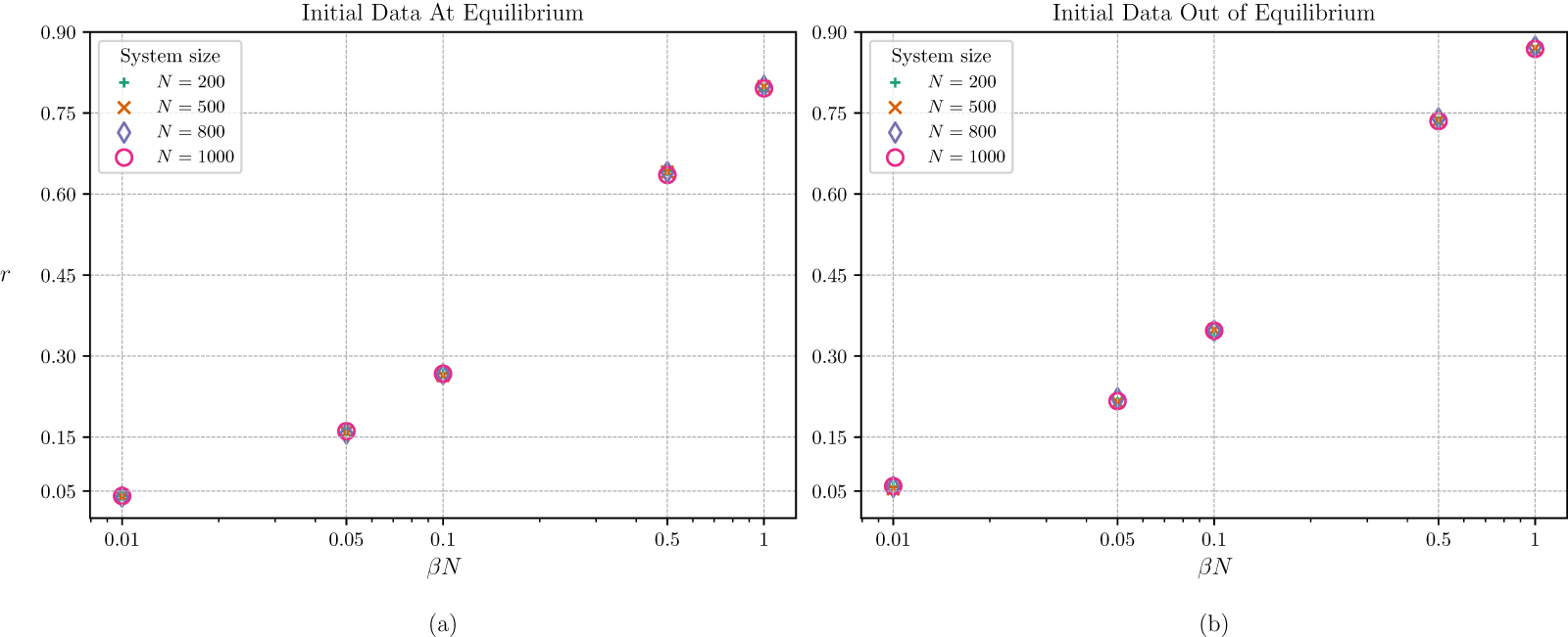
Ratio  $r$ as a function of
 $\beta N$ for
 $N = 200$,
 $500$,
 $800$ and
 $1000$, with initial conditions (a) at thermal equilibrium with (4.6) and (b) out of thermal equilibrium with (4.7).

1 Long description
Two scatter plots labeled (a) and (b). The horizontal axis in both plots is labeled beta N, ranging from 0.01 to 1. The vertical axis is labeled r, ranging from 0 to 0.90. In plot (a), titled Initial Data At Equilibrium, the data points are plotted for different system sizes: N equals 200, N equals 500, N equals 800 and N equals 1000. The legend indicates different markers for each system size: plus for N equals 200, cross for N equals 500, diamond for N equals 800 and circle for N equals 1000. The data points show a trend where r increases with beta N, with values approximately at (0.01, 0.04), (0.05, 0.16), (0.1, 0.27), (0.5, 0.64) and (1, 0.80). In plot (b), titled Initial Data Out of Equilibrium, the same system sizes and markers are used. The trend is similar to plot (a), with r increasing as beta N increases. The data points are approximately at (0.01, 0.06), (0.05, 0.22), (0.1, 0.35), (0.5, 0.74) and (1, 0.87). Both plots demonstrate that the values of r collapse for the same value of beta N irrespective of the system size.
Figure 1 plots the computed values of  $r$ from the two initial conditions (4.6) and (4.7) for different values of
 $\beta$ and
 $N$. In particular, we choose
 $N = 200$,
 $500$,
 $800$ and
 $1000$, and for each
 $N$ corresponding values of
 $\beta$ to make
 $\beta N=1$,
 $0.5$,
 $0.1$,
 $0.05$ and
 $0.01$. We see from Figure 1 that all results of
 $r$ collapse for the same value of
 $\beta N$ irrespective of the value of
 $N$, which is true for both initial conditions. This means that the relative contributions from non-resonant terms are indeed controlled by the parameter
 $\beta N$ as indicated by the theory. In addition, we see that for large values of
 $\beta N$, say
 $\beta N=1$, the contribution from non-resonant terms can rise up to
 $O(80\%)$ for both initial conditions. Clearly for these cases, ignoring the non-resonant terms (i.e., applying the normal form transformation inconsistently) leads to excessive errors to the dynamics of the system.
5. Conclusion
We have derived a rigorous upper bound on the non-linearity parameter  $\beta$ as
 $\beta\ll 1/N^{1+\epsilon}$, which guarantees the normal form transformation for the
 $\beta$-FPUT system to remain bounded and near-identity. This validity condition suggests a parameter
 $\beta N$, which controls the relative importance of the non-resonant cubic terms in the dynamical evolution equation. We further design numerical experiments to verify this condition by applying a sixth-order symplectic integrator method to the dynamical equation. We show that for both initial conditions at thermal equilibrium and out-of-equilibrium, the relative contribution of non-resonant terms in the Hamiltonian is indeed governed by
 $\beta N$ as indicated by the theory. Beyond a clarification of the validity condition, our work provides a practical criterion to select
 $\beta$ and
 $N$ with awareness of the effect of non-resonant terms for future studies of FPUT dynamics. The methodology to achieve so can also be extended to normal form transformations in other non-linear Hamiltonian systems with cubic non-linearities. Furthermore, the present results provide a rigorous justification for employing normal-form transformations to extend the derivation of the WKE from the reduced evolution equation of the
 $\beta$-FPUT system [Reference Wu27] to the full
 $\beta$-FPUT dynamics, offering a route parallel to the direct derivation for the full system recently obtained in [Reference Vassilev and Wu26].
Author contributions
Conceptualization: B.W., M.O. and Y.P. Methodology: B.W., Y.P. and Z.H. Writing original draft: B.W. and Y.P. All authors approved the final submitted draft.
Funding statement
This research was supported by Simons Collaboration on Wave Turbulence, Grant No. 617006 and NSF grants DMS-1936640 and DMS-2350242. M.O. is also supported by INFN (MMNLP and FieldTurb). Computational resources and services were provided by Advanced Research Computing (ARC) at the University of Michigan, including the Great Lakes high-performance computing cluster.
Competing interests
None.
Ethical standards
The research meets all ethical guidelines, including adherence to the legal requirements of the study country.
Appendix A. Proof of Theorem 3.1
To prove Theorem 3.1, we separate the sums in the canonical transformation (2.7) into three cases with respect to the  $\delta(\cdot)$ functions and find upper bounds for the sums. Note that all
 $k's$ are positive as defined in (2.3).
Case 1:  $k_1-k_2-k_3-k_4 \equiv 0 \text{ } \text{(mod } N)$. Then we may have three possibilities.
1.
$k_1-k_2-k_3-k_4=0$, then we have:
(A.1)\begin{align}
&\omega_{k_1}-\omega_{k_2}-\omega_{k_3}-\omega_{k_4}=2\left[\sin{\left(\frac{\pi k_1}{N}\right)}-\sin{\left(\frac{\pi k_2}{N}\right)}-\sin{\left(\frac{\pi k_3}{N}\right)}-\sin{\left(\frac{\pi k_4}{N}\right)}\right]\\ notag
&=4\left[\sin{\left(\frac{\pi (k_1-k_2)}{2N}\right)}\cos{\left(\frac{\pi (k_1+k_2)}{2N}\right)}-\sin{\left(\frac{\pi (k_3+k_4)}{2N}\right)}\cos{\left(\frac{\pi (k_3-k_4)}{2N}\right)}\right]\\ notag
&=4\sin{\left(\frac{\pi (k_1-k_2)}{2N}\right)}\left[\cos{\left(\frac{\pi (k_1+k_2)}{2N}\right)}-\cos{\left(\frac{\pi (k_3-k_4)}{2N}\right)}\right]\\ notag
&=8\sin{\left(\frac{\pi (k_1-k_2)}{2N}\right)}\sin{\left(\frac{\pi (k_1+k_2+k_3-k_4)}{4N}\right)}\sin{\left(\frac{\pi (k_3-k_4-k_1-k_2)}{4N}\right)}\\ notag
&=8\sin{\left(\frac{\pi (k_1-k_2)}{2N}\right)}\sin{\left(\frac{\pi (k_1-k_4)}{2N}\right)}\sin{\left(\frac{\pi (k_3-k_1)}{2N}\right)}.\end{align}We must have
$k_2,k_3,k_4 \lt k_1$ with at least one of
$k_i \sim k_1$ in the restriction of
$k_1-k_2-k_3-k_4=0$. Then for fixed
$k_1$, there are
$O(k_1^2)$ choices for
$(k_2,k_3,k_4)$. We choose a constant
$C =\frac{1}{3}$. Without loss of generality suppose
$k_2 \geq Ck_1$, then
$k_1-k_2=k_3+k_4 \geq \max(k_3,k_4)$,
$k_1-k_3=k_2+k_4\geq Ck_1$ and similarly
$k_1-k_4\geq Ck_1$. Then we have:
(A.2)\begin{equation}
\left|A^{(1)}\right|^2 \lesssim \frac{\left(\frac{ k_1}{N}\right)^2\left(\frac{\max(k_3,k_4)}{N}\right)^2}{\left(\frac{\max(k_3,k_4)}{N}\right)^2\left(\frac{Ck_1}{N}\right)^4} \lesssim \frac{N^2}{k_1^2}.
\end{equation}Then we know that:
(A.3)\begin{equation}
\sum_{k_1-k_2-k_3-k_4=0}\left|A^{(1)}\right|^2 \lesssim \frac{N^2}{k_1^2}\cdot k_1^2 = N^2.
\end{equation}2.
$k_1-k_2-k_3-k_4=-2N$, then we can do a change of variable:
$k_1' = N-k_1, k_2' = N-k_2, k_3'=N-k_3, k_4'=N-k_4$, we then get:
$k_1'-k_2'-k_3'-k_4'=(N-k_1)-(N-k_2)-(N-k_3)-(N-k_4)=-k_1+k_2+k_3+k_4-2N = 0$. And we still have
$\sin\left(\frac{\pi k_i}{N}\right)=\sin\left(\frac{\pi k'_i}{N}\right)$. Then applying the result from the last case, we can get:
(A.4)\begin{equation}
\sum_{k_1-k_2-k_3-k_4=-2N}\left|A^{(1)}\right|^2 \lesssim N^2.
\end{equation}3.
$k_1-k_2-k_3-k_4=-N$, without loss of generality suppose
$\frac{N|h|}{\pi}=|k_1-k_4|\leq|k_1-k_2|,|k_1-k_3|$,
$k_2 \leq k_3$, then we can write
$\frac{\pi k_1}{N}=y,\frac{\pi k_4}{N}=y+h,\frac{\pi k_2}{N}=x,\frac{\pi k_3}{N}=\pi-x-h$, which gives:
\begin{equation*}\frac{\pi}{N}(k_1-k_2-k_3-k_4) = y-x-(\pi-x-h)-(y+h)=-\pi.\end{equation*}Then now we have:
(A.5)\begin{align}
&\left|\sin{\left(\frac{\pi k_1}{N}\right)}-\sin{\left(\frac{\pi k_2}{N}\right)}-\sin{\left(\frac{\pi k_3}{N}\right)}-\sin{\left(\frac{\pi k_4}{N}\right)}\right|\\ notag
=&\left|\sin(y)-\sin(y+h)-\sin(x)-\sin(\pi-x-h)\right|\\ notag
\geq&\Big||\sin(y)-\sin(y+h)|-|\sin(x)+\sin(x+h)|\Big|\\ notag
=&2\Bigg|\left|\cos\left(y+\frac{h}{2}\right)\sin\left(\frac{h}{2}\right)\right|-\left|\sin\left(x+\frac{h}{2}\right)\cos\left(\frac{h}{2}\right)\right|\Bigg|.\end{align}Since we assume
$k_2\leq k_3$, we have:
$x\leq\pi-x-h \lt \pi$, which then gives
$\frac{|h|}{2} \lt x+\frac{h}{2}\leq \frac{\pi}{2}$. It means that:
\begin{equation*}\sin\left(\frac{|h|}{2}\right) \lt \sin\left(x+\frac{h}{2}\right).\end{equation*}On the other hand, if
$y\geq\frac{\pi}{2}$, then we must have
$\frac{\pi}{2}\leq y-|h|\leq\pi$ or
$\frac{\pi}{2}\leq y+|h|\leq\pi$. Similarly, if
$y \lt \frac{\pi}{2}$, then we must have
$0\leq y-|h| \lt \frac{\pi}{2}$ or
$0\leq y+|h|\leq\frac{\pi}{2}$. Otherwise either
$k_1 \gt \frac{N}{2},k_2,k_3,k_4 \leq \frac{N}{2}$ or
$k_1\leq \frac{N}{2}, k_2,k_3,k_4 \gt \frac{N}{2}$, which neither give
$k_1-k_2-k_3-k_4=-N$. It then means that
$|h| \lt \frac{\pi}{2}$ and
\begin{equation*}0\leq\left|\cos\left(y+\frac{h}{2}\right)\right|\leq\left|\cos\left(\frac{h}{2}\right)\right|.\end{equation*}Then we further get:
(A.6)\begin{equation}
(A.5) \gt rsim \cos\left(\frac{h}{2}\right)\left|\sin\left(x+\frac{h}{2}\right)-\sin\left(\frac{|h|}{2}\right)\right|.
\end{equation}(i) If
$h \gt 0$, then we have
$\frac{x+h}{2}=\frac{1}{2}(x+\frac{h}{2})+\frac{h}{4}\leq \frac{3}{8}\pi$, and:
then we can bound
\begin{equation*}(A.5) \gt rsim \cos\left(\frac{x+h}{2}\right) \sin\left(\frac{x}{2}\right) \gt rsim \sin\left(\frac{x}{2}\right),\end{equation*}
$\left|A^{(1)}\right|^2$ as:
(A.7)\begin{equation}
\left|A^{(1)}\right|^2 \lesssim \frac{\sin(x)\sin(y)\sin(y+h)}{\sin^2\left(\frac{x}{2}\right)} \lesssim \frac{\sin(y)\sin(y+h)}{\sin\left(\frac{x}{2}\right)}.
\end{equation}In this case, since
$x+\frac{h}{2}\leq \frac{\pi}{2}$, then
$x \lt \frac{\pi}{2}$. We either have:
$\pi-x-h\leq y-h$, which then gives
$\frac{\pi}{2} \lt \pi-x\leq y$ and
$\frac{\sin(y)}{\sin(\frac{x}{2})}=\frac{2\sin(y)\cos(\frac{x}{2})}{\sin(x)}\lesssim 1$, or have:
$\frac{\pi}{2} \gt x\geq y+h$, and
$\frac{\sin(y+h)}{\sin(\frac{x}{2})}=\frac{2\sin(y+h)\cos(\frac{x}{2})}{\sin(x)}\lesssim 1$. Hence we can get
$\left|A^{(1)}\right|^2 \lesssim 1$ for
$h \gt 0$.(ii) If
$h = 0$, then
(A.8)\begin{equation}
\left|A^{(1)}\right|^2 \lesssim 1.
\end{equation}(iii) If
$h \lt 0$, then we have
$\frac{x}{2}\leq\frac{\pi}{4}+\frac{|h|}{4}\leq \frac{3}{8}\pi$, and:
then we can bound
\begin{equation*}(A.5) \gt rsim \sin\left(\frac{x+h}{2}\right) \cos\left(\frac{x}{2}\right) \gt rsim \sin\left(\frac{x+h}{2}\right) ,\end{equation*}
$\left|A^{(1)}\right|^2$ as:
(A.9)\begin{equation}
\left|A^{(1)}\right|^2 \lesssim \frac{\sin(x+h)\sin(y)\sin(y+h)}{\sin^2\left(\frac{x+h}{2}\right)} \lesssim \frac{\sin(y)\sin(y+h)}{\sin\left(\frac{x+h}{2}\right)}.
\end{equation}Similarly, since
$x+\frac{h}{2}\leq \frac{\pi}{2}$, then
$x+h \lt \frac{\pi}{2}$. We either have:
$\frac{\pi}{2} \lt \pi-x-h\leq y-|h|=y+h$, which then gives
$\frac{\sin(y+h)}{\sin(\frac{x+h}{2})}\lesssim 1$, or have:
$x\geq y+|h|$, i.e.,
$\frac{\pi}{2} \gt x+h\geq y$ and
$\frac{\sin(y)}{\sin(\frac{x+h}{2})}\lesssim 1$. Hence we can get
$\left|A^{(1)}\right|^2 \lesssim 1$ for
$h \lt 0$.
Let
$\mathbb{Z}_N:=N^{-1}\mathbb{Z}$. Thus we can get the estimate for the sum:
(A.10)\begin{equation}
\sum_{k_1-k_2-k_3-k_4=-N}\left|A^{(1)}\right|^2 \lesssim \sum_{h\in \mathbb{Z}_N \cap (0,1)} \sum_{x\in \mathbb{Z}_N \cap (0,1)} 1\lesssim N^2.
\end{equation}





From the above cases, we have:
 \begin{equation}
\sum_{k_1-k_2-k_3-k_4 \equiv 0 \text{ } \text{(mod } N)}\left|A^{(1)}\right|^2 \lesssim N^2.
\end{equation}
Case 2:  $k_1-k_2+k_3+k_4 \equiv 0 \text{ } \text{(mod } N)$. Then we again have three possibilities.
1.
$k_1-k_2+k_3+k_4 = 0$. Similarly as Case 1(1), we have:
(A.12)and\begin{align}
&\omega_{k_1}-\omega_{k_2}+\omega_{k_3}+\omega_{k_4}\\ notag
&=8\sin{\left(\frac{\pi (k_2-k_1)}{2N}\right)}\sin{\left(\frac{\pi (k_2-k_3)}{2N}\right)}\sin{\left(\frac{\pi (k_2-k_4)}{2N}\right)}\end{align}
$k_1,k_3,k_4 \lt k_2$. Similarly, we choose a constant
$C \lt \frac{1}{3}$. Without loss of generality, suppose
$k_1 \geq Ck_2$, then
$k_2-k_1 = k_3+k_4$,
$k_2-k_4=k_1+k_3\geq k_1\geq Ck_2$, and similarly
$k_2-k_3\geq Ck_2$, then we have
(A.13)\begin{equation}
\left|A^{(2)}\right|^2 \lesssim \frac{\left(\frac{1}{N}\right)^4k_1k_2k_3k_4}{\left(\frac{C k_2}{N}\right)^4\left(\frac{k_3+k_4}{N}\right)^2} \lesssim \frac{N^2}{k_2^2}.
\end{equation}Then we can calculate the sum:
(A.14)\begin{equation}
\sum_{k_1-k_2+k_3+k_4=0}\left|A^{(2)}\right|^2 \lesssim \sum_{k_2=1}^{N-1}\sum_{k_3=1}^{k_2}\frac{N^2}{k_2^2} \lesssim N^2\log N.
\end{equation}2.
$k_1-k_2+k_3+k_4 = 2N$. Then similarly as Case 1(2), we can change of variables:
$k_i'=N-k_i$ for
$i\in \{1,2,3,4\}$. Then we can obtain the same result as (1):
(A.15)\begin{equation}
\sum_{k_1-k_2+k_3+k_4=2N}\left|A^{(2)}\right|^2 \lesssim N^2\log N.
\end{equation}3.
$k_1-k_2+k_3+k_4 = N$. We apply the same technique as in Case 1(3) and we can conclude:
(A.16)\begin{equation}
\sum_{k_1-k_2+k_3+k_4=N}\left|A^{(2)}\right|^2 \lesssim N^2.
\end{equation}





Thus we have:
 \begin{equation}
\sum_{k_1-k_2+k_3+k_4 \equiv 0 \text{ } \text{(mod } N)}\left|A^{(2)}\right|^2 \lesssim N^2 \log N.
\end{equation}
Case 3:  $k_1+k_2+k_3+k_4 \equiv 0 \text{ } \text{(mod } N)$
Let  $M:=\max\left(\sin{\left(\frac{\pi k_1}{N}\right)},\sin{\left(\frac{\pi k_2}{N}\right)},\sin{\left(\frac{\pi k_3}{N}\right)},\sin{\left(\frac{\pi k_4}{N}\right)}\right)\leq 1$, and
 $\qquad m:=\min\left(\sin{\left(\frac{\pi k_1}{N}\right)},\sin{\left(\frac{\pi k_2}{N}\right)},\sin{\left(\frac{\pi k_3}{N}\right)},\sin{\left(\frac{\pi k_4}{N}\right)}\right)$.
Then we know that:
 \begin{equation}
\left|A^{(3)}\right|^2 \lesssim \frac{mM^3}{M^2} \lesssim 1.
\end{equation}
Thus we have:
 \begin{equation}
\sum_{k_1+k_2+k_3+k_4 \equiv 0 \text{ } \text{(mod } N)}\left|A^{(3)}\right|^2 \lesssim N^2.
\end{equation}
Therefore, we have proved Theorem 3.1.




 Open access

