1 Introduction
The dynamic interactions between fluid flows and arrays of slender structures play an important role in a broad range of physical processes. In nature, the metachronal motion of dense arrays of cilia serve a number of crucial physiological functions, from cell propulsion (den Toonder & Onck Reference den Toonder and Onck2013) to particle regulation (Masoud & Alexeev Reference Masoud and Alexeev2011). In industrial applications, bioinspired designs based on slender structures are finding uses in areas such as flow control (Favier et al. Reference Favier, Dauptain, Basso and Bottaro2009; Kunze & Brücker Reference Kunze and Brücker2012) and sensing (Kottapalli et al. Reference Kottapalli, Bora, Asadnia, Miao, Venkatraman and Triantafyllou2016). Furthermore, the interactions between vegetation and fluid flows have important consequences in terms of agriculture (de Langre Reference de Langre2008) and coastal protection (Gedan et al. Reference Gedan, Kirwan, Wolanski, Barbier and Silliman2011).
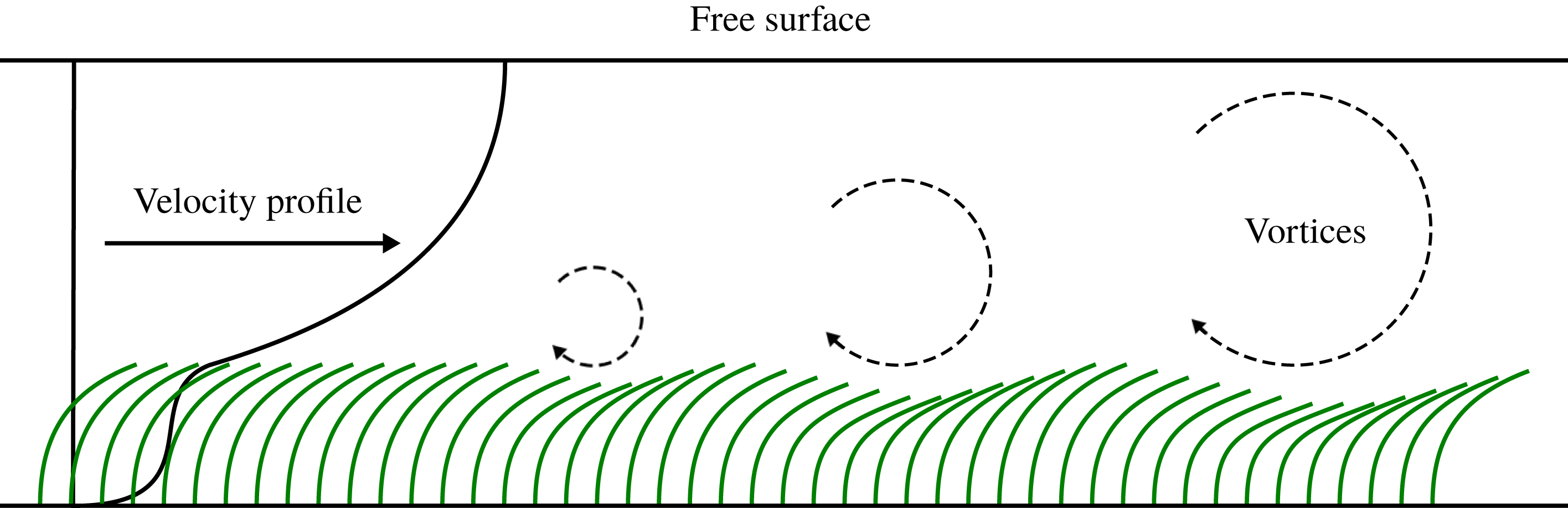
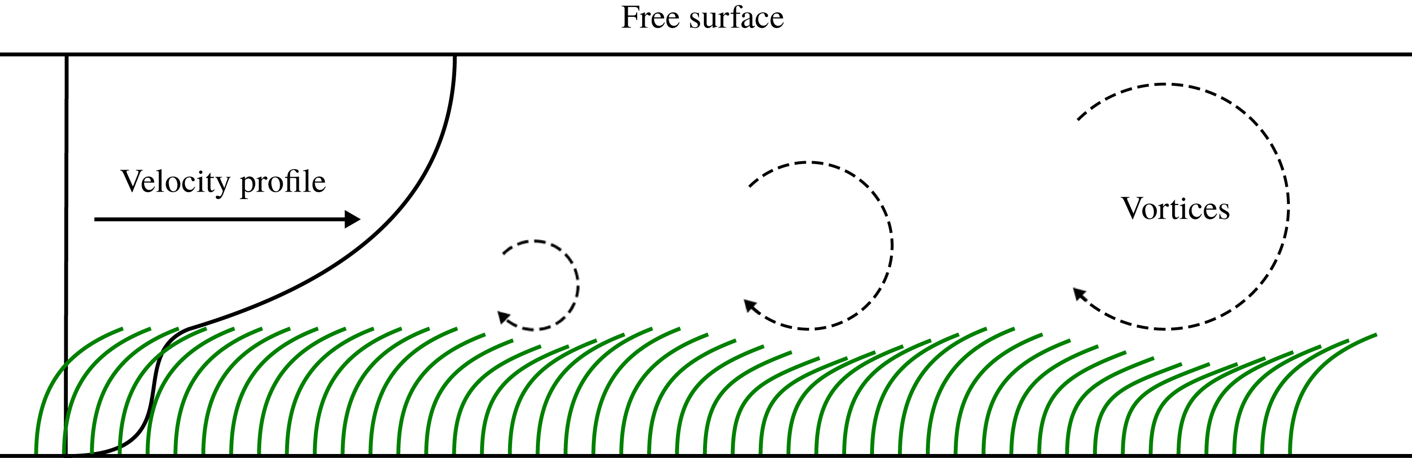
In vegetative flows, the emergence of coherent waving motions between adjacent plants is known to appear under certain conditions. This phenomenon is known as honami for terrestrial flows, and monami for aquatic flows. This behaviour is initiated by the discontinuity in drag between the interstitial flow within the canopy and the bulk flow over the top of the canopy, which produces an inflection point within the velocity profile (Nepf Reference Nepf2012b ). The inflection point makes the flow susceptible to Kelvin–Helmholtz instabilities, which roll up to form coherent vortical structures and propagate through the array (Ghisalberti Reference Ghisalberti2002). The passage of the vortices over individual plants causes a local deflection, which propagates through the canopy with the flow structures. This is observed as a travelling wave through the array, as shown in figure 1.
Velocity profile and monami motion over a submerged canopy.
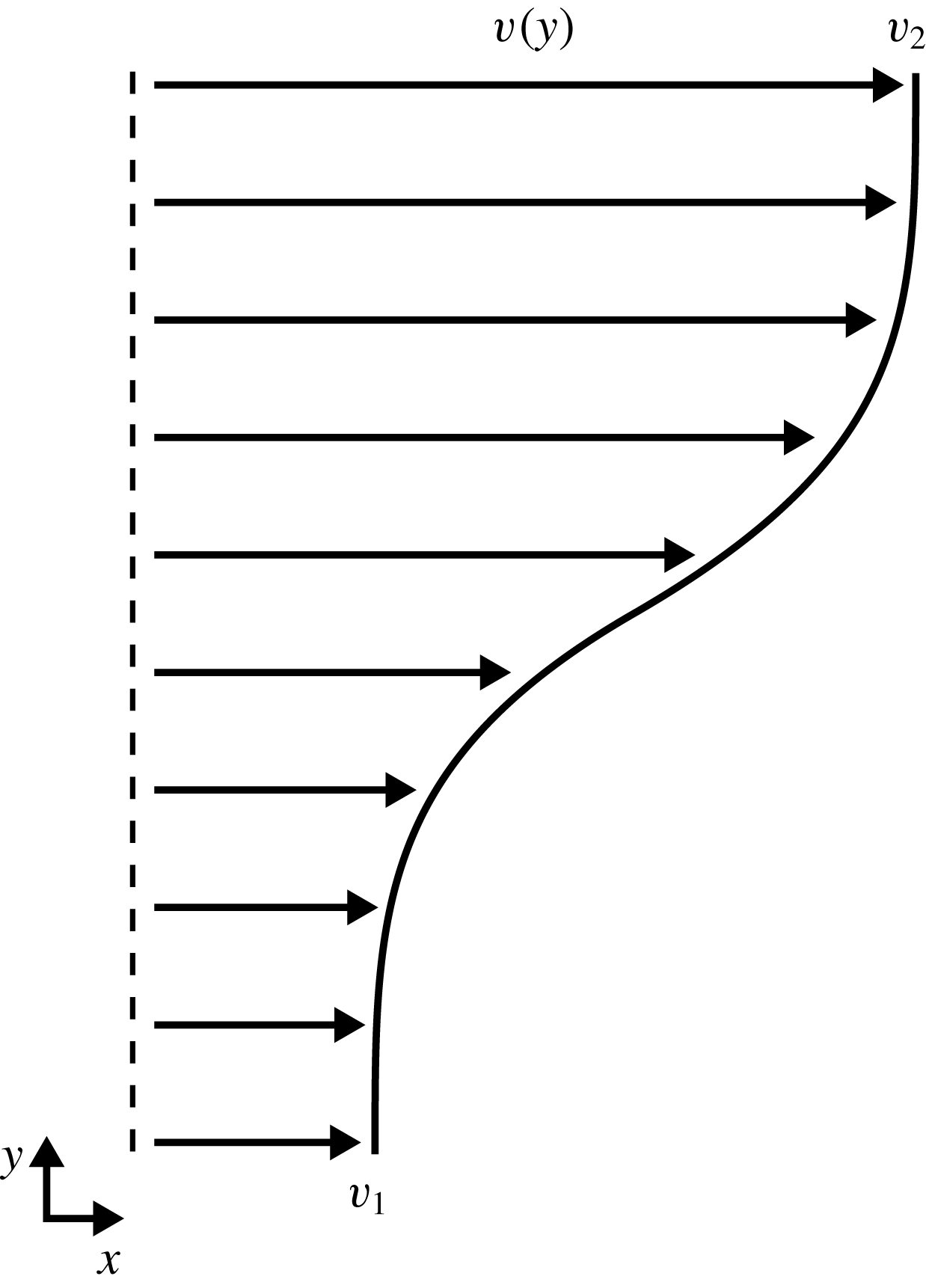
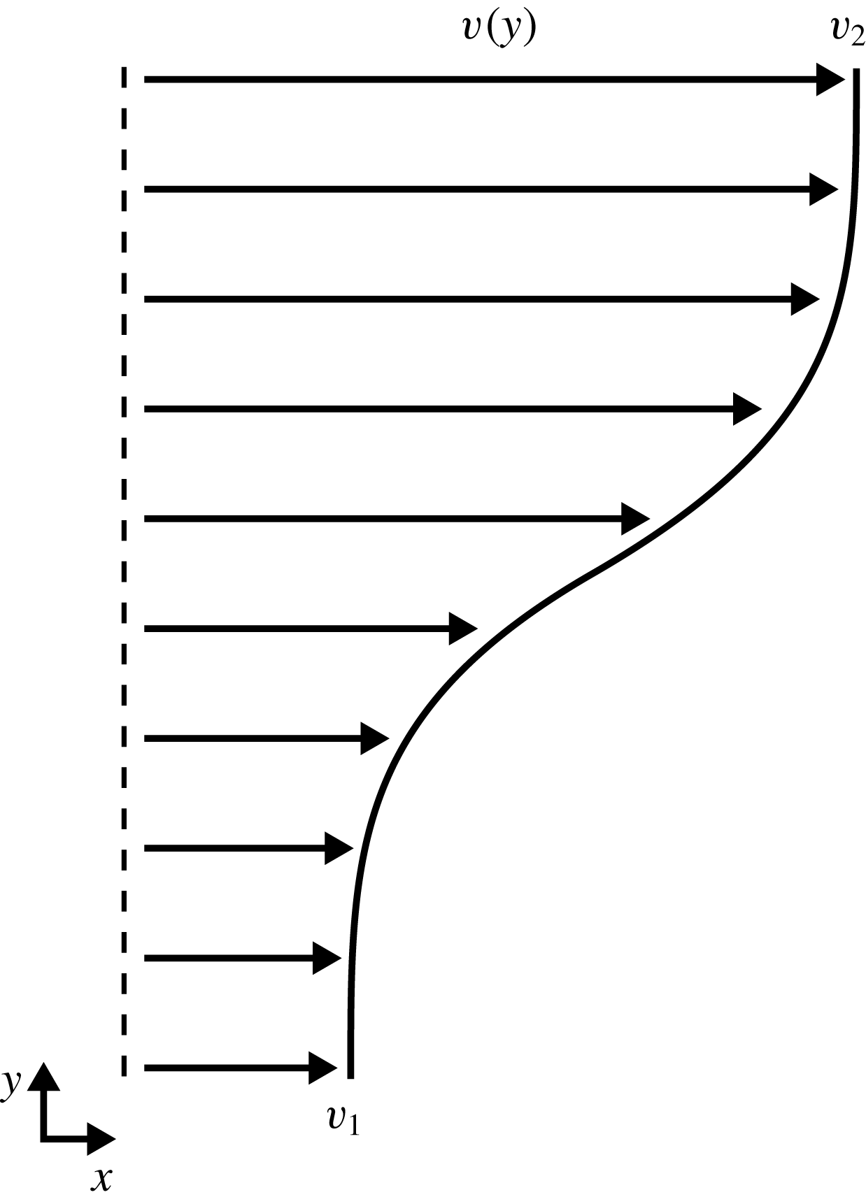
Ghisalberti (Reference Ghisalberti2002) argued that the honami/monami effect is primarily governed by the mixing layer instability, and that the waving motion is a forced response to the Kelvin–Helmholtz vortices which are generated due to the inflectional velocity profile. To support this, Ghisalberti performed experiments on a scaled seagrass model which indicated strong correlations between the velocity spectra, waving frequency and predicted frequency of the Kelvin–Helmholtz vortices, estimated as
 $$\begin{eqnarray}f_{KH}=St_{n}\left(\frac{v_{1}+v_{2}}{2\unicode[STIX]{x1D703}}\right),\end{eqnarray}$$
where
 $St_{n}$
is the natural Strouhal number associated with mixing layers,
 $\unicode[STIX]{x1D703}$
is the momentum thickness and
 $v_{1}$
and
 $v_{2}$
are the low- and high-stream velocities (see figure 2). Through theory and experiment, the natural Strouhal number is known to be approximately
 $St_{n}\approx 0.032$
(Ho & Huerre Reference Ho and Huerre1984). The momentum thickness is given by
 $$\begin{eqnarray}\unicode[STIX]{x1D703}=\int _{-\infty }^{\infty }\left[\frac{1}{4}-\left(\frac{v-\frac{1}{2}\left(v_{1}+v_{2}\right)}{v_{2}-v_{1}}\right)^{2}\right]\!\text{d}y.\end{eqnarray}$$
Ghisalberti (Reference Ghisalberti2002) also noted that the observed waving frequencies were much lower than the natural frequencies of the model plants. However, in this case the values quoted for the natural frequency of the plant models suggest that the theoretical undamped natural frequency was used for comparison. In the case of structures immersed in a flow, the damped natural frequency can be significantly lower.
More recent studies have suggested that the structural properties do in fact play a role in the waving instability. Py, de Langre & Moulia (Reference Py, de Langre and Moulia2004) developed a simplified fluid model combined with a flexible porous layer for the canopy. While the main instability mechanism was driven by the Kelvin–Helmholtz instability, the model indicated that the characteristics of this instability are significantly modified when the canopy compliance is considered. In subsequent work, Py et al. (Reference Py, de Langre, Moulia and Hémon2005), Py, de Langre & Moulia (Reference Py, de Langre and Moulia2006) used an image-correlation technique to extract the wavelengths and frequencies of the coherent structures over two different plant species: alfalfa and wheat. These two species were selected as they share similar geometric properties (height and spacing) but different material properties (density and stiffness), and therefore different natural frequencies. Interestingly, for both species, the waving motion was found to occur near their own (damped) natural frequency. Moreover, this was observed over the full range of tested wind speeds. Extending their previous model, Py et al. observed a lock-in effect with increasing wind speed as the frequency of the Kelvin–Helmholtz instability approached the natural frequency of the canopy.
A similar lock-in effect has been observed in flow control applications, where arrays of slender structures are used to augment the wake topology behind bluff bodies. Favier et al. (Reference Favier, Dauptain, Basso and Bottaro2009) used a homogenised porous layer model to examine the effect of a row of passive flaps attached to the aft of a circular cylinder. Under optimum conditions, they observed drag reductions of 15 % and reductions in the lift fluctuations of 40 %, which they attributed to a stabilisation of the wake. In the optimal regime, they observed a travelling wave through the array with a frequency that matched the vortex shedding frequency. Several other studies have also observed this travelling wave, and many report a lock-in at optimal conditions between the travelling wave frequency and the shedding frequency (Kunze & Brücker Reference Kunze and Brücker2012; Mazellier, Feuvrier & Kourta Reference Mazellier, Feuvrier and Kourta2012; Venkataraman & Bottaro Reference Venkataraman and Bottaro2012).
While several studies have observed these coherent waving interactions, the mechanisms which govern this behaviour are not yet fully understood. This is partly due to the complexity of the coupled behaviour, but also partly due to the large parameter space that governs this process. Previous studies have indicated a dependence on structural material properties (Py et al.
Reference Py, de Langre and Moulia2006), spatial density and distribution (Ghisalberti & Nepf Reference Ghisalberti and Nepf2006), submergence ratio (Nepf & Vivoni Reference Nepf and Vivoni2000), flow speed (Ghisalberti Reference Ghisalberti2002) and Reynolds number (Singh et al.
Reference Singh, Bandi, Mahadevan and Mandre2016). With this in mind, to help form a fundamental understanding of this phenomenon, an idealised numerical test case is formulated consisting of a large array of regularly spaced slender structures in a two-dimensional (2-D) open-channel flow. Furthermore, the parameter space is restricted so that only the structural properties (mass density and Young’s modulus) are varied, while everything else is held constant. This decision is made based on previous studies (Py et al.
Reference Py, de Langre and Moulia2006; Gosselin & de Langre Reference Gosselin and de Langre2009), which suggest a strong dependence of the waving instability on the ratio between the natural frequencies of the mixing layer instability and canopy. By manipulating the structural properties this ratio can be varied without affecting other important parameters, such as the length of the flaps or the cross-flow Reynolds number. A direct modelling approach, whereby the individual structures and their dynamics are fully resolved, is realised via a lattice Boltzmann-immersed boundary-finite element model. For steady flow conditions at low–moderate Reynolds number (
 $Re=80$
), the dynamic response of the array is measured for a range of structural material properties. Both the mass ratio and bending rigidity are varied over a range spanning two orders of magnitude, and the ensuing response is characterised and quantified.
The restriction of the parameter space, while necessary, limits the applicability of the present work. Perhaps the most notable limitation is the restriction to two dimensions. When compared to a 2-D structure with an effective infinite width, the blockage effect (drag) of a 3-D structure is significantly reduced, owing to the out-of-plane flow around the structure. Furthermore, while shallow submerged canopies tend to generate Kelvin–Helmholtz vortices which remain predominantly lateral to the canopy, the coherent flow structures generated in terrestrial and deeply submerged canopies tend to be highly three-dimensional, due to interactions with the upper boundary layer turbulence (Nepf Reference Nepf2012a ). Nevertheless, the restriction to two dimensions is a useful simplification to form a basis of understanding and there are many examples of similar fundamental studies (Ikeda, Yamada & Toda Reference Ikeda, Yamada and Toda2001; Gosselin & de Langre Reference Gosselin and de Langre2009; Singh et al. Reference Singh, Bandi, Mahadevan and Mandre2016). The following sections provide details and validation of the fully coupled numerical model. After introducing the case, results are then presented and the main findings discussed, with a particular focus on the coupled waving instability and its associated lock-in.
2 Methods
2.1 Lattice Boltzmann method
The lattice Boltzmann method (LBM) has evolved over recent years to become an attractive alternative to the Navier–Stokes equations. Derived from kinetic theory, the LBM relies on a mesoscopic description of the fluid to compute its macroscopic behaviour (Chen & Doolen Reference Chen and Doolen1998; Aidun & Clausen Reference Aidun and Clausen2010). The driving equation behind the LBM is the Boltzmann equation, which in its discrete form is given by
 $$\begin{eqnarray}f_{i}(\boldsymbol{x}+\boldsymbol{c}_{i}\unicode[STIX]{x0394}t,t+\unicode[STIX]{x0394}t)-f_{i}(\boldsymbol{x},t)=\frac{\unicode[STIX]{x0394}t}{\unicode[STIX]{x1D70F}}\left[f_{i}^{eq}(\boldsymbol{x},t)-f_{i}(\boldsymbol{x},t)\right]+\unicode[STIX]{x0394}tF_{i}(\boldsymbol{x},t),\end{eqnarray}$$
where
 $\boldsymbol{x}$
are the spatial coordinates,
 $t$
is time,
 $\boldsymbol{c}_{i}$
is the
 $i$
th component of the lattice velocity vector and
 $F_{i}(\boldsymbol{x},t)$
is an external force discretised on the lattice. The probability distribution function,
 $f_{i}(\boldsymbol{x},t)$
, describes the proportion of fluid molecules within an elemental volume located at
 $\boldsymbol{x}$
and time
 $t$
moving with velocity
 $\boldsymbol{c}_{i}$
. Equation (2.1) can be split into two steps: a streaming step, where the components of the distribution function propagate through the lattice along discrete velocity links; and a collision step, where the distribution function relaxes towards a local equilibrium. The relaxation time scale,
 $\unicode[STIX]{x1D70F}$
, is related to the (lattice) viscosity via
 $$\begin{eqnarray}\unicode[STIX]{x1D708}=\left(\unicode[STIX]{x1D70F}-{\textstyle \frac{1}{2}}\right)c_{s}^{2},\end{eqnarray}$$
where
 $c_{s}$
is the lattice speed of sound. The equilibrium function,
 $f_{i}^{eq}(\boldsymbol{x},t)$
, is a function of local macroscopic quantities only, and can be obtained via a Taylor series (He & Luo Reference He and Luo1997a
,Reference He and Luo
b
) or Hermite polynomial (Shan & He Reference Shan and He1998; Shan, Yuan & Chen Reference Shan, Yuan and Chen2006) expansion of the Maxwell–Boltzmann distribution, giving
 $$\begin{eqnarray}f_{i}^{eq}(\boldsymbol{x},t)=w_{i}\unicode[STIX]{x1D70C}\left(1+\frac{\boldsymbol{c}_{i}\boldsymbol{\cdot }\boldsymbol{v}}{c_{s}^{2}}+\frac{(\boldsymbol{c}_{i}\boldsymbol{\cdot }\boldsymbol{v})^{2}}{2c_{s}^{4}}-\frac{\boldsymbol{v}\boldsymbol{\cdot }\boldsymbol{v}}{2c_{s}^{2}}\right),\end{eqnarray}$$
where
 $w_{i}$
is a velocity-specific weighting factor related to the discrete lattice. The macroscopic quantities,
 $\unicode[STIX]{x1D70C}(\boldsymbol{x},t)$
and
 $\boldsymbol{v}(\boldsymbol{x},t)$
, can be calculated by taking the leading moments of the distribution function, as given by
 $$\begin{eqnarray}\displaystyle & \displaystyle \unicode[STIX]{x1D70C}(\boldsymbol{x},t)=\mathop{\sum }_{i}f_{i}(\boldsymbol{x},t) & \displaystyle\end{eqnarray}$$
 $$\begin{eqnarray}\displaystyle & \displaystyle \unicode[STIX]{x1D70C}\boldsymbol{v}(\boldsymbol{x},t)=\mathop{\sum }_{i}\boldsymbol{c}_{i}f_{i}(\boldsymbol{x},t)+\frac{\unicode[STIX]{x0394}t}{2}\boldsymbol{f}(\boldsymbol{x},t). & \displaystyle\end{eqnarray}$$
The force density,
 $\boldsymbol{f}(\boldsymbol{x},t)$
, is crucial for the present work as it provides the coupling between the fluid and structural dynamics. Its Cartesian form is discretised on the lattice to give (Guo, Zheng & Shi Reference Guo, Zheng and Shi2002)
 $$\begin{eqnarray}F_{i}(\boldsymbol{x},t)=w_{i}\left(1-\frac{1}{2\unicode[STIX]{x1D70F}}\right)\left(\frac{\boldsymbol{c}_{i}-\boldsymbol{v}}{c_{s}^{2}}+\frac{\boldsymbol{c}_{i}\boldsymbol{\cdot }\boldsymbol{v}}{c_{s}^{4}}\,\boldsymbol{c}_{i}\right)\boldsymbol{\cdot }\boldsymbol{f}(\boldsymbol{x},t).\end{eqnarray}$$
2.2 Finite element method
The present model adopts the corotational formulation of the finite element method (FEM) to solve the structural dynamics. The main idea of the corotational formulation is to decompose the motion of each element within the assemblage into a rigid body motion and a purely deformational one (de Borst et al. Reference de Borst, Crisfield, Remmers and Verhoosel2012). This is achieved by adopting two reference configurations: the initial (or reference) frame, and the corotated (or local) frame which is attached to the element and moves with it (De Rosis et al. Reference De Rosis, Falcucci, Ubertini and Ubertini2013). The rigid body motion is measured with respect to the initial configuration and can be arbitrarily large. On the other hand, the elemental deformation is measured with respect to the corotated frame and is assumed to be small within the local frame (Goza & Colonius Reference Goza and Colonius2017). In this regard, two sets of quantities are defined: the local quantities which are measured with respect to the corotated frame, and the global quantities which are measured with respect to the global coordinate system. In the formulation of the system matrices which appear in the governing equations, the elemental matrices are first calculated in the corotated frame, after which they are transformed to the global coordinate frame, and then finally assembled into the global system matrices.
The present work adopts two-noded Euler–Bernoulli beam elements to discretise the flaps. The key assumption in this formulation is that the cross-sections of the beam do not deform and remain plane and normal to the neutral axis. This implies there is no transverse shear through the beam and therefore limits the validity of the current model to slender structures. Each node contains three degrees of freedom (two translational and one rotational). While this approach does consider flap extensibility, for the configurations of interest in the present work the axial extension is negligible compared to the bending deformation.
Following Bathe (Reference Bathe2014), the equilibrium conditions governing the nonlinear Newton–Raphson solution are
 $$\begin{eqnarray}\displaystyle & \displaystyle \unicode[STIX]{x1D648}\ddot{\boldsymbol{U}}^{n+1,k}+\unicode[STIX]{x1D646}^{n+1,k}\unicode[STIX]{x0394}\boldsymbol{U}^{k}=\boldsymbol{F}_{ext}^{n+1}-\boldsymbol{F}_{int}^{n+1,k} & \displaystyle\end{eqnarray}$$
 $$\begin{eqnarray}\displaystyle & \displaystyle \boldsymbol{U}^{n+1,k+1}=\boldsymbol{U}^{n+1,k}+\unicode[STIX]{x0394}\boldsymbol{U}^{k}, & \displaystyle\end{eqnarray}$$
where
 $n$
and
 $k$
are the time step and iteration counters,
 $\unicode[STIX]{x1D648}$
is the mass matrix,
 $\unicode[STIX]{x1D646}$
is the tangent stiffness matrix,
 $\boldsymbol{F}_{ext}$
is the external load vector (including fluid forces),
 $\boldsymbol{F}_{int}$
are the internal forces (due to the stress) within the structure,
 $\ddot{\boldsymbol{U}}$
are the nodal accelerations and
 $\unicode[STIX]{x0394}\boldsymbol{U}$
are the incremental nodal displacements.
To advance in time, the constant-average-acceleration version of the Newmark integration scheme is used in conjunction with an iterative Newton–Raphson procedure (Zienkiewicz, Taylor & Zhu Reference Zienkiewicz, Taylor and Zhu2013). Once the incremental displacements,
 $\unicode[STIX]{x0394}\boldsymbol{U}^{k}$
, are found, the displacement at the next iteration is calculated via (2.8) and the tangent stiffness matrix and internal forces are updated. The iteration scheme is converged once the incremental displacements become sufficiently small, after which the solution is advanced to the next time step (Zienkiewicz, Taylor & Fox Reference Zienkiewicz, Taylor and Fox2014).
2.3 Immersed boundary method
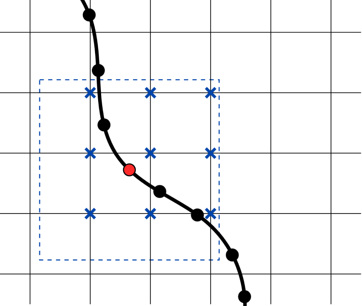
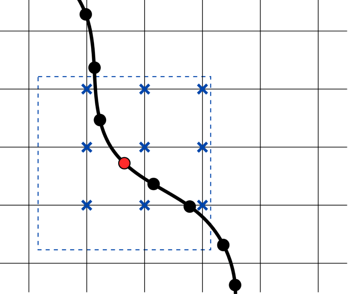
The immersed boundary method (IBM) provides the link between the fluid and structural dynamics. It relies on two separate grids to represent the fluid and the boundary, which are independent of each other and non-conforming (Mittal & Iaccarino Reference Mittal and Iaccarino2005), as shown in figure 3. The fluid is defined on an Eulerian grid (the lattice), which is Cartesian and fixed in space. The boundary, on the other hand, is represented on a Lagrangian grid, which is curvilinear and free to move across the computational domain. The main idea of the IBM is to mimic the effect of the boundary by introducing a source term (force) in the governing fluid equations. These forces are calculated in such a way so that the fluid feels the presence of the boundary through this force, and the no-slip condition is satisfied along the surface.
Support stencil for IBM marker. Dashed line is the support stencil over which the interpolation/spreading steps are performed. Crossed lattice sites are the support points that exist within the support stencil and are directly involved in the grid-to-grid communication.
Since the two grids are separate from each other, communication between them is crucial. Moreover, since they are non-conforming, this data transfer requires specialised interpolation/spreading operators. Specifically, the momentum field must be interpolated from the fluid grid (Eulerian) to the boundary grid (Lagrangian), and the resulting forces must be spread back from the boundary grid to the fluid grid. The operators defining these communication steps are given by (Peskin Reference Peskin2002)
 $$\begin{eqnarray}\displaystyle & \displaystyle \unicode[STIX]{x1D6F7}(\boldsymbol{X})={\mathcal{I}}[\unicode[STIX]{x1D719}(\boldsymbol{x})]=\mathop{\sum }_{\unicode[STIX]{x1D6FA}_{s}}\unicode[STIX]{x1D719}(\boldsymbol{x})\;\tilde{\unicode[STIX]{x1D6FF}}(\boldsymbol{x}-\boldsymbol{X})\unicode[STIX]{x0394}x\unicode[STIX]{x0394}y\unicode[STIX]{x0394}z & \displaystyle\end{eqnarray}$$
 $$\begin{eqnarray}\displaystyle & \displaystyle \unicode[STIX]{x1D719}(\boldsymbol{x})={\mathcal{S}}[\unicode[STIX]{x1D6F7}(\boldsymbol{X})]=\mathop{\sum }_{\unicode[STIX]{x1D6E4}_{s}}\unicode[STIX]{x1D6F7}(\boldsymbol{X})\;\tilde{\unicode[STIX]{x1D6FF}}(\boldsymbol{x}-\boldsymbol{X})\unicode[STIX]{x1D716}\unicode[STIX]{x0394}q\unicode[STIX]{x0394}r\unicode[STIX]{x0394}s, & \displaystyle\end{eqnarray}$$
where
 $\boldsymbol{x}=(x,y,z)$
,
 $\boldsymbol{X}=(q,r,s)$
,
 $\unicode[STIX]{x1D719}$
is a quantity defined in the Eulerian frame,
 $\unicode[STIX]{x1D6F7}$
is the same quantity defined in the Lagrangian frame and
 $\unicode[STIX]{x1D716}$
is a scaling factor which ensures reciprocity between the interpolation and spreading steps (Pinelli et al.
Reference Pinelli, Naqavi, Piomelli and Favier2010). Here, lower-case notation denotes values in the Eulerian frame, and upper-case notation denotes values in the Lagrangian frame. The present work adopts the three-point version of the discrete Dirac delta function,
 $\tilde{\unicode[STIX]{x1D6FF}}$
, proposed by Roma, Peskin & Berger (Reference Roma, Peskin and Berger1999).
The full LBM–IBM algorithm is given by Li et al. (Reference Li, Favier, D’Ortona and Poncet2016) and makes use of the fact that the LBM forcing scheme (Guo et al. Reference Guo, Zheng and Shi2002) decomposes the velocity into a predicted and a force-corrected term (Wu & Shu Reference Wu and Shu2009). After one pass of the LBM equations, the macroscopic fluid velocity can be written
 $$\begin{eqnarray}\unicode[STIX]{x1D70C}\boldsymbol{v}(\boldsymbol{x},t)=\unicode[STIX]{x1D70C}\boldsymbol{v}^{\ast }(\boldsymbol{x},t)+\frac{\unicode[STIX]{x0394}t}{2}\boldsymbol{f}(\boldsymbol{x},t),\end{eqnarray}$$
where
 $\boldsymbol{v}^{\ast }$
is the predicted velocity field. The density and predicted velocity field are the only known quantities at this stage. Since the fluid velocity at the boundary must equal the velocity of the boundary,
 $\boldsymbol{V}={\mathcal{I}}[\boldsymbol{v}]$
, then converting equation (2.11) into the Lagrangian frame gives
 $$\begin{eqnarray}{\mathcal{I}}[\unicode[STIX]{x1D70C}(\boldsymbol{x},t)]\boldsymbol{V}(\boldsymbol{X},t)={\mathcal{I}}[\unicode[STIX]{x1D70C}\boldsymbol{v}^{\ast }(\boldsymbol{x},t)]+\frac{\unicode[STIX]{x0394}t}{2}\boldsymbol{F}(\boldsymbol{X},t).\end{eqnarray}$$
Since the velocity of the boundary,
 $\boldsymbol{V}$
, is known, equation (2.12) can be rearranged and solved for the corrective force density,
 $\boldsymbol{F}$
. The force is then transferred back to the Eulerian frame via the spreading operator,
 ${\mathcal{S}}$
. Finally, the velocity field is updated by adding the corrective force to the predicted velocity field (2.11).
2.4 Fluid–structure coupling
The present model adopts a partitioned approach to solving the interaction between the fluid and structure, whereby separate field solvers are used to calculate the fluid and structural dynamics and the necessary interfacial quantities – displacements, velocities and forces – are transferred between the two solvers as required. For problems where the density ratio between the structure and fluid (
 $\unicode[STIX]{x1D70C}_{s}/\unicode[STIX]{x1D70C}_{f}$
) is
 $O(1)$
or lower, partitioned schemes are known to suffer from instabilities generated at the interface, known as added-mass instabilities (Förster, Wall & Ramm Reference Förster, Wall and Ramm2007; van Brummelen Reference van Brummelen2009). Without special treatment in the coupling scheme these instabilities can severely impact the stability and accuracy of the solution. To overcome this, the present model adopts a strongly coupled block Gauss–Seidel implicit coupling scheme. This technique iterates over the separate field solvers within the time step until the kinematic and dynamic interface compatibility conditions are met (Hou, Wang & Layton Reference Hou, Wang and Layton2012; Degroote Reference Degroote2013). However, this does not guarantee stability and the coupling scheme may still converge slowly. Therefore, after each iteration the solution is relaxed by combining the structural displacements at the current and previous iterations, such that
 $$\begin{eqnarray}\tilde{\boldsymbol{U}}=\unicode[STIX]{x1D714}\boldsymbol{U}+(1-\unicode[STIX]{x1D714})\tilde{\boldsymbol{U}}^{k-1},\end{eqnarray}$$
where
 $\tilde{\boldsymbol{U}}$
is the relaxed solution which is passed to the fluid solver,
 $\boldsymbol{U}$
is the displacement computed from the structural FEM solver and
 $\tilde{\boldsymbol{U}}^{k-1}$
is the solution from the previous iteration.
To accelerate the convergence of the coupling scheme, the relaxation factor is adjusted dynamically according to Aitken’s delta-squared method (Küttler & Wall Reference Küttler and Wall2008; Degroote Reference Degroote2013)
 $$\begin{eqnarray}\unicode[STIX]{x1D714}^{k}=-\unicode[STIX]{x1D714}^{k-1}\frac{(\boldsymbol{r}^{k-1})^{T}(\boldsymbol{r}^{k}-\boldsymbol{r}^{k-1})}{|\boldsymbol{r}^{k}-\boldsymbol{r}^{k-1}|^{2}},\end{eqnarray}$$
where
 $\boldsymbol{r}^{k}$
is the residual vector, which is also used as a stopping criterion for the sub-iteration scheme
 $$\begin{eqnarray}\boldsymbol{r}^{k}=\boldsymbol{U}^{k}-\tilde{\boldsymbol{U}}^{k-1}.\end{eqnarray}$$
In general, decreasing the structure-to-fluid density ratio will require more sub-iterations to properly satisfy the interface conditions. For the range of values tested in the present work the coupling scheme was found to converge within approximately 2–7 sub-iterations, depending on the particular case and simulation state.
3 Validation
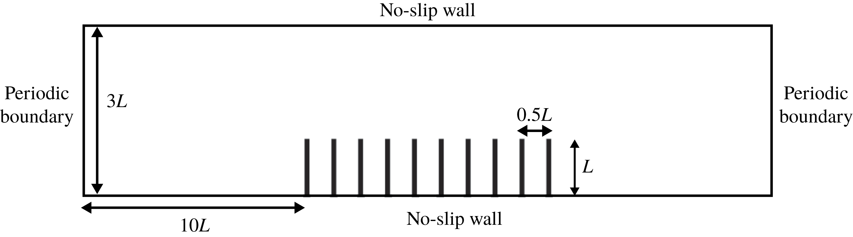
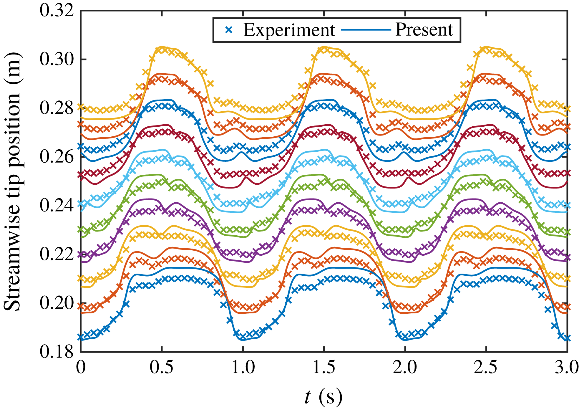
The present numerical model has been extensively validated in previous work (Favier et al. Reference Favier, Li, Kamps, Revell, O’Connor and Brücker2017; Harwood et al. Reference Harwood, O’Connor, Muñoz, Santasmasas and Revell2018). However, for the purpose of the present work a brief validation is also presented here. The model is tested against experimental data obtained for an oscillating channel flow with a row of 10 wall-mounted flexible flaps (Favier et al. Reference Favier, Li, Kamps, Revell, O’Connor and Brücker2017). A schematic of the computational set-up is shown in figure 4. In the original experiment, the flaps spanned most of the channel width and therefore the flow can be considered two-dimensional at the channel centreline. For more details regarding the experimental set-up, the reader is referred to Favier et al. (Reference Favier, Li, Kamps, Revell, O’Connor and Brücker2017).
Schematic of computational domain for validation case.
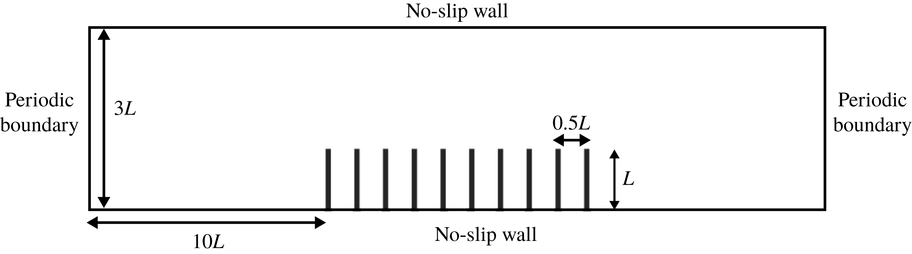
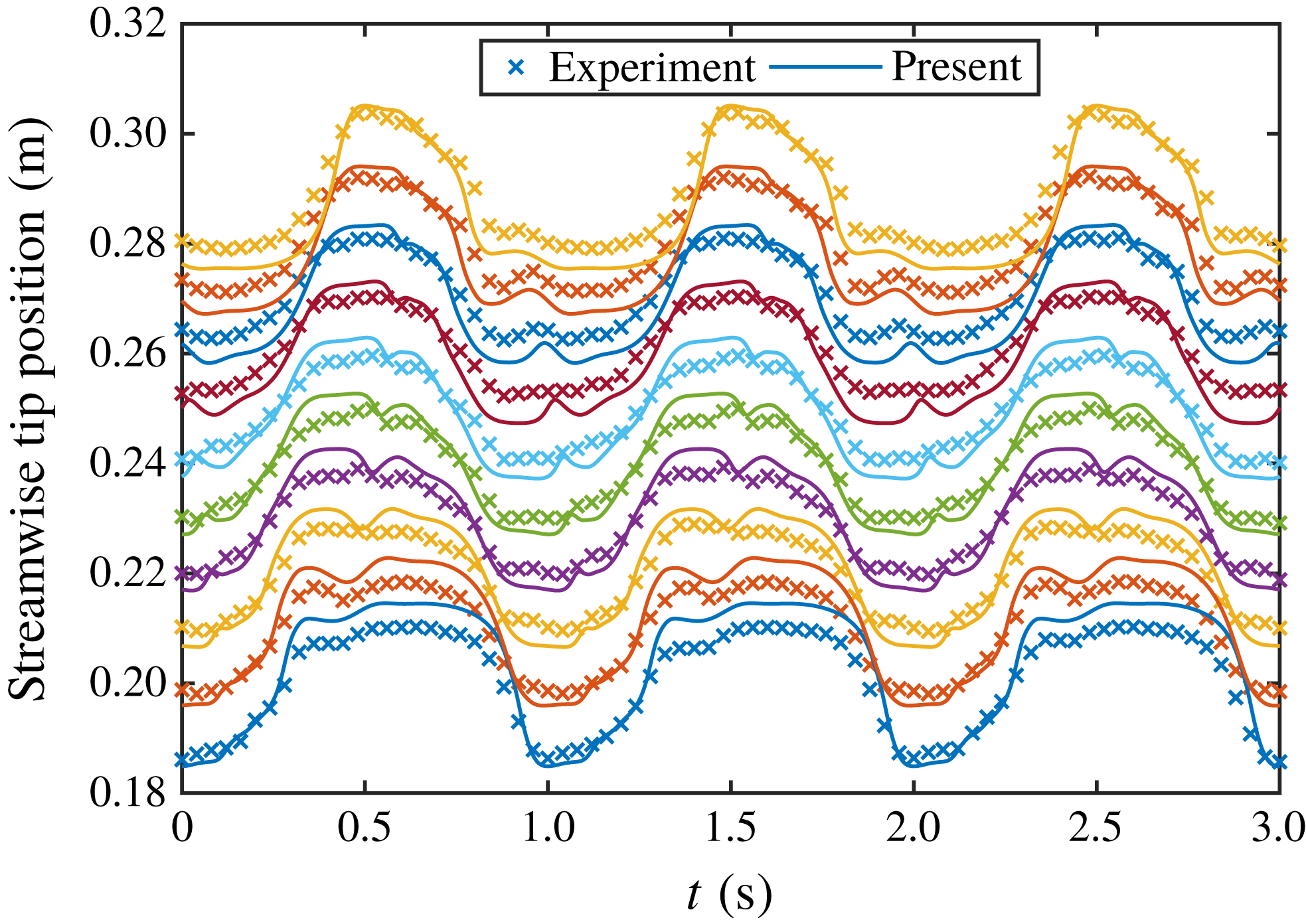
Figure 5 shows the experimental and numerical results for the streamwise tip deflection of each flap. Overall the agreement is good; however, some slight discrepancies are observed. These may be attributed to differences in the approximation of the experimental parameters. In particular, the bending rigidity of the flaps is extremely sensitive to the flap thickness, with
 $EI\propto h^{3}$
. Another possible explanation for the noted differences is 3-D effects, due to the finite span of the flaps in the experiment, which are not captured in the 2-D simulation. Nevertheless, the agreement is good and, as such, verifies the ability of the present model to reproduce the dynamic motion of multiple wall-mounted flexible flaps.
Validation of present model. Streamwise tip positions for each flap are compared against the experiment of Favier et al. (Reference Favier, Li, Kamps, Revell, O’Connor and Brücker2017).
4 Simulation set-up
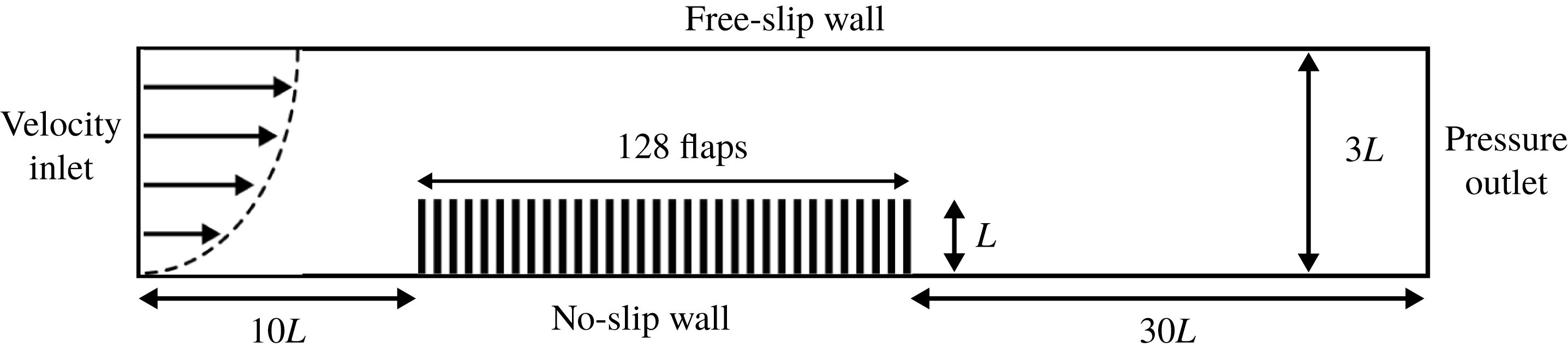
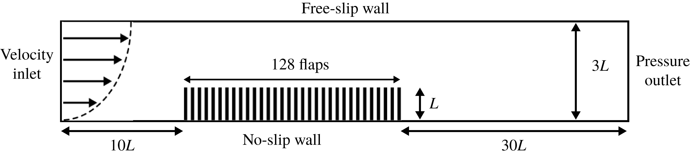
To limit the edge effects and isolate the waving instability, a large array of flaps is tested. Figure 6 shows a schematic of the computational domain. The set-up consists of an open-channel flow with an array of 128 wall-mounted flexible flaps. The flaps have a length
 $L$
and are equally spaced by
 $0.5L$
. The spacing was chosen based on previous work examining the coherent interactions of wall-mounted flexible flaps (Favier et al.
Reference Favier, Li, Kamps, Revell, O’Connor and Brücker2017; Revell et al.
Reference Revell, O’Connor, Sarkar, Li, Favier, Kamps and Brücker2017). Due to the 2-D nature of this work and the variability in spacing of real vegetation, a direct comparison of spacing is inappropriate. A more common metric is the solid volume fraction occupied by the flaps/vegetation, which for the present configuration is
 $\unicode[STIX]{x1D719}=0.04$
. Nepf (Reference Nepf2012a
) provides typical solid volume fractions for various species of real aquatic vegetation, with seagrasses (
 $\unicode[STIX]{x1D719}\approx 0.01{-}0.1$
) most resembling the present configuration. The channel height is given by
 $H=3L$
, so that the configuration resembles that of a shallow submerged vegetation canopy (Nepf Reference Nepf2012a
). The inlet is placed
 $10L$
upstream from the array, whereas the outlet is placed
 $30L$
downstream. Preliminary tests indicated this was sufficient to limit the effect of the boundaries on the global behaviour of the array and is in line with other studies of wall-mounted flaps at similar Reynolds numbers (Lee et al.
Reference Lee, Park, Kim, Ryu and Sung2017; Lee, Park & Sung Reference Lee, Park and Sung2018).
The inlet velocity profile is set according to
 $$\begin{eqnarray}v_{x}(0,y,t)=1.5\bar{v}\frac{y(2H-y)}{H^{2}},\end{eqnarray}$$
where
 $\bar{v}$
is the mean (bulk) velocity. Zero-velocity initial conditions are set and the inlet velocity is ramped up over a short period of time. This limits the appearance of density waves, which arise due to the weakly compressible nature of the LBM. A fixed pressure is set at the outlet, no-slip on the bottom wall and a free-slip (rigid lid) condition is used for the top boundary (Dupont et al.
Reference Dupont, Gosselin, Py, de Langre, Hemon and Brunet2010). Based on the bulk velocity and flap length the Reynolds number is 80. This was chosen from a preliminary study, which indicated this is close to the minimum Reynolds number capable of exhibiting waving instabilities.
Schematic of computational domain.
For a fixed Reynolds number and geometry the governing parameters are the dimensionless mass ratio and bending stiffness, given by
 $$\begin{eqnarray}{\mathcal{M}}=\frac{\unicode[STIX]{x1D70C}_{s}h}{\unicode[STIX]{x1D70C}_{f}L},\quad {\mathcal{K}}=\frac{EI}{\unicode[STIX]{x1D70C}_{f}\bar{v}^{2}L^{3}},\end{eqnarray}$$
where
 $\unicode[STIX]{x1D70C}_{f}$
and
 $\unicode[STIX]{x1D70C}_{s}$
are the fluid and structural densities,
 $L$
is the flap length,
 $h$
is the flap thickness,
 $E$
is the Young’s modulus and
 $I$
is the second area moment of the flap. The reduced velocity,
 ${\mathcal{U}}=\sqrt{{\mathcal{M}}/{\mathcal{K}}}$
, is also commonly adopted for studying fluid-structure interaction problems. However, the purpose of the present work is to examine the effect of the mechanical properties of the flaps (mass density and Young’s modulus) for a fixed flow condition. Since the reduced velocity is a function of both of these properties, the dimensionless mass ratio and bending stiffness are considered to be more suitable for separating the individual effects of these two properties.
In the following tests, five different mass ratios (denoted M1–5) and ten different bending rigidities (K1–10) are tested. An initial parameter search identified an appropriate range where a variety of behaviours were observed. These values are distributed in powers of ten, such that
 $$\begin{eqnarray}\displaystyle & \displaystyle \text{M}m=1\times 10^{-1+((m-1)/2)},\quad m=1\ldots 5 & \displaystyle\end{eqnarray}$$
 $$\begin{eqnarray}\displaystyle & \displaystyle \text{K}k=5\times 10^{-3+(2(k-1)/9)},\quad k=1\ldots 10. & \displaystyle\end{eqnarray}$$
Gosselin & de Langre (Reference Gosselin and de Langre2009) show that the characteristics of the waving instability are broadly similar for both aquatic and terrestrial vegetation. However, they also note some distinct differences, particularly with regards to the region of the parameter space where lock-in appears, which they attribute to the large discrepancies in mass ratio. As an example, in terrestrial vegetation the density ratio (
 $\unicode[STIX]{x1D70C}_{s}/\unicode[STIX]{x1D70C}_{f}$
) is typically O (1000), whereas for aquatic vegetation
 $O(1)$
is common. Given that the vegetation slenderness ratio (
 $L/h$
) is usually O (100), this equates to a mass ratio of O (10) for terrestrial vegetation (corresponding to M5 in (4.3)) and O (0.01) for aquatic vegetation (one order of magnitude below M1). As discussed in § 2.4, there are significant modelling challenges associated with the very low mass ratios that govern the behaviour of aquatic vegetation and so the parameter space is restricted here. In regards to the non-dimensional bending stiffness, de Langre (Reference de Langre2008) gives a Young’s modulus of
 $10^{8}$
Pa for living vegetal tissue. Assuming a flow speed of
 $10~\text{m}~\text{s}^{-1}$
for terrestrial vegetation and
 $1~\text{m}~\text{s}^{-1}$
in the aquatic case, this equates to a non-dimensional bending stiffness of O (0.1) and O (0.01) for terrestrial and aquatic vegetation, respectively. Therefore, the present work captures most of the parameter space that governs the behaviour of both aquatic and terrestrial vegetation.
To compare the instability mechanism of the array, a similar range of tests are performed for a single flap. Since the instability mechanism in this case is different to that observed for the array, preliminary tests found that the range of mass ratio given in (4.3) did not yield significant dynamic motion for the single flap. Therefore, the range of mass ratio in the single flap tests is shifted one order of magnitude higher. To keep the numbering scheme consistent, the range of mass ratios in the single flap tests are given by
 $$\begin{eqnarray}\text{M}m=1\times 10^{-1+((m-1)/2)},\quad m=3\ldots 7.\end{eqnarray}$$
Therefore, both the single and array cases at
 $\text{M}m\text{K}k$
share the same material properties.
Each flap is discretised with 50 IBM markers/lattice sites (
 $\unicode[STIX]{x0394}x=0.02L$
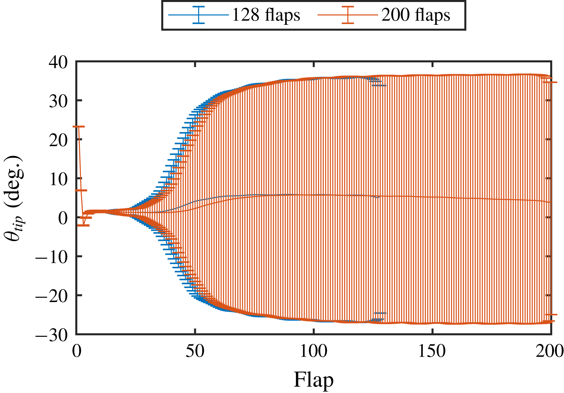
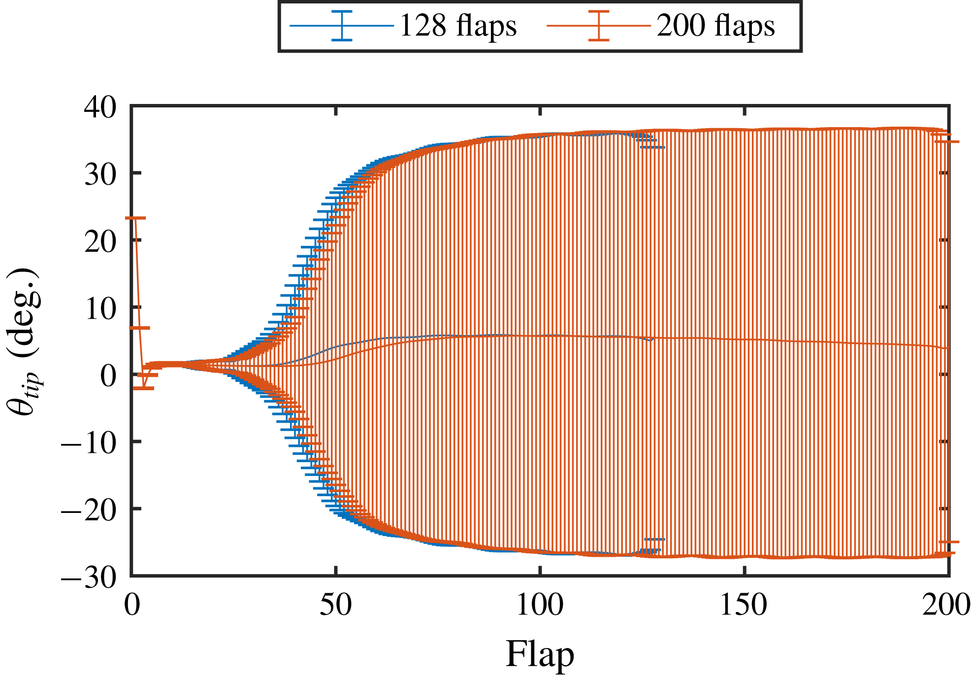
) and 20 FEM elements. To ensure a configuration-independent solution, tests were performed on both the array length and the grid resolution. Figure 7 shows the range of tip motion for each flap along the array for a representative case (M3K8) with 128 and 200 flaps. The tip angle is measured from the base of the flap as the angle between the flap tip and its equilibrium position, so that
 $\unicode[STIX]{x1D703}_{tip}=\arctan (\unicode[STIX]{x1D6FF}_{x}/(L+\unicode[STIX]{x1D6FF}_{y}))$
, where
 $\unicode[STIX]{x1D6FF}_{x}$
and
 $\unicode[STIX]{x1D6FF}_{y}$
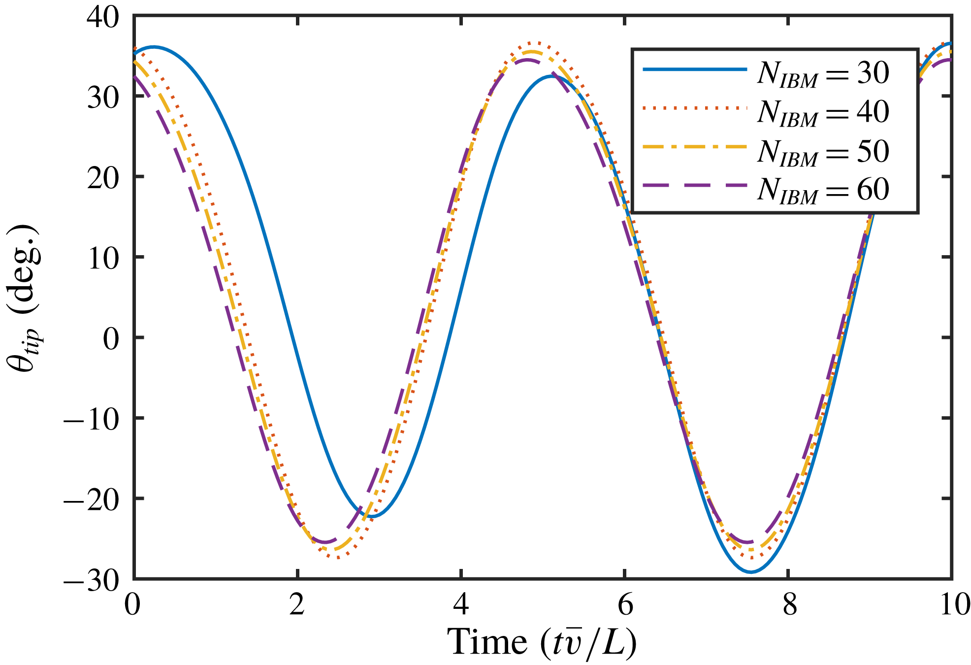
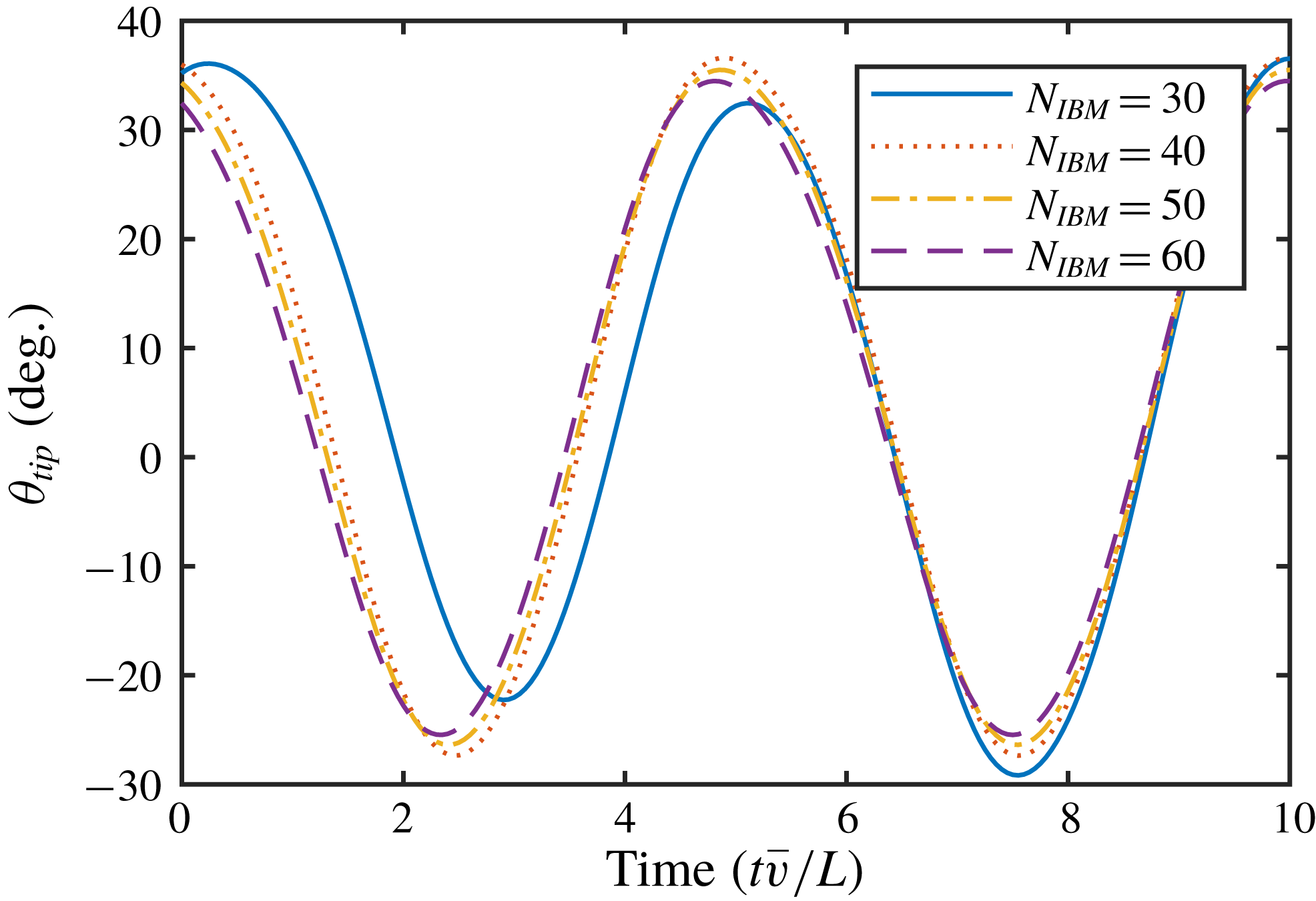
are the tip deflections. As can be seen, there is little difference between the two cases in terms of the range of tip motion. Furthermore, there is little variation in the tip motion in the extended region of the array (flaps 129 to 200). Although there is a slight decreasing trend in the mean value towards the end of the array, this is relatively minor and the range of motion seems unaffected. For this reason, 128 flaps was deemed sufficient for the length of the array. Figure 8 shows the tip deflection for a representative flap (number 100) for a range of tested grid resolutions. After a relatively large shift in solution between the
 $N_{IBM}=30$
and
 $N_{IBM}=40$
cases, there is little change with further increasing grid resolution. As such, the
 $N_{IBM}=50$
resolution was selected for all further simulations.
5 Dynamic response and characterisation of behaviour
5.1 Classification of states for single flap
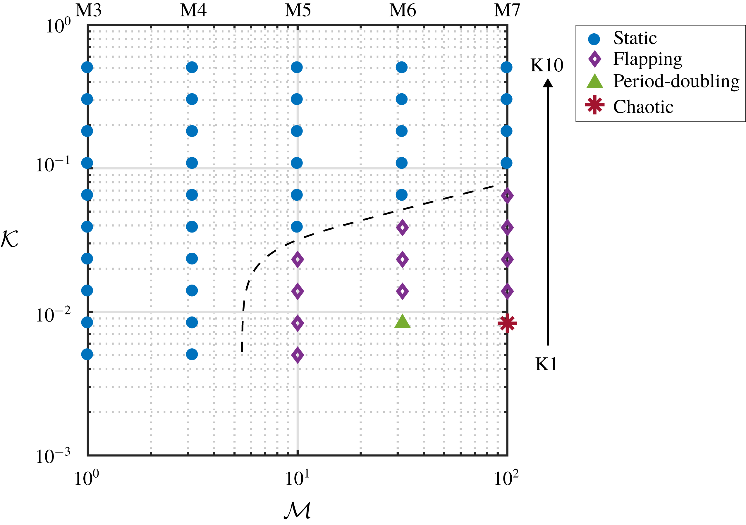
Initially, to provide a contrast to the system of multiple flaps, the response of a single wall-mounted flap is investigated. As mentioned in § 4, the range of tested mass ratios for the single flap cases are shifted one order of magnitude higher (M3–7) compared to the array cases (M1–5). Through observation of the response, each case is classified into one of four modes: static, flapping, period doubling or chaotic motion. Figure 9 shows the parameter map for all tested cases (M3–7, K1–10). Note that cases where large mass ratios were combined with low bending rigidities (M6K1, M7K1), the large flapping motion resulted in the flap making contact with the bottom wall or passing straight through it. While this did not always result in stability problems (e.g. when the contact was brief), no contact model is incorporated in the present model and so results were not collected for these cases. This also happened for the M7K2 case; however, the period of time before contact was made was deemed sufficient to characterise the motion.
Minimum, maximum and time-averaged flap deflection (expressed as tip angle) across the array for two different configurations (128 and 200 flaps).
Tip angle history of the 100th flap over the final 10 seconds of simulation, where
 $N_{IBM}$
is the number of IBM markers/lattice sites used to discretise the flap.
Parameter map with observed behaviour modes for single flap. Dashed line is shown to help distinguish boundaries. The range of mass ratio and bending stiffness is given by M3–7 and K1–10.
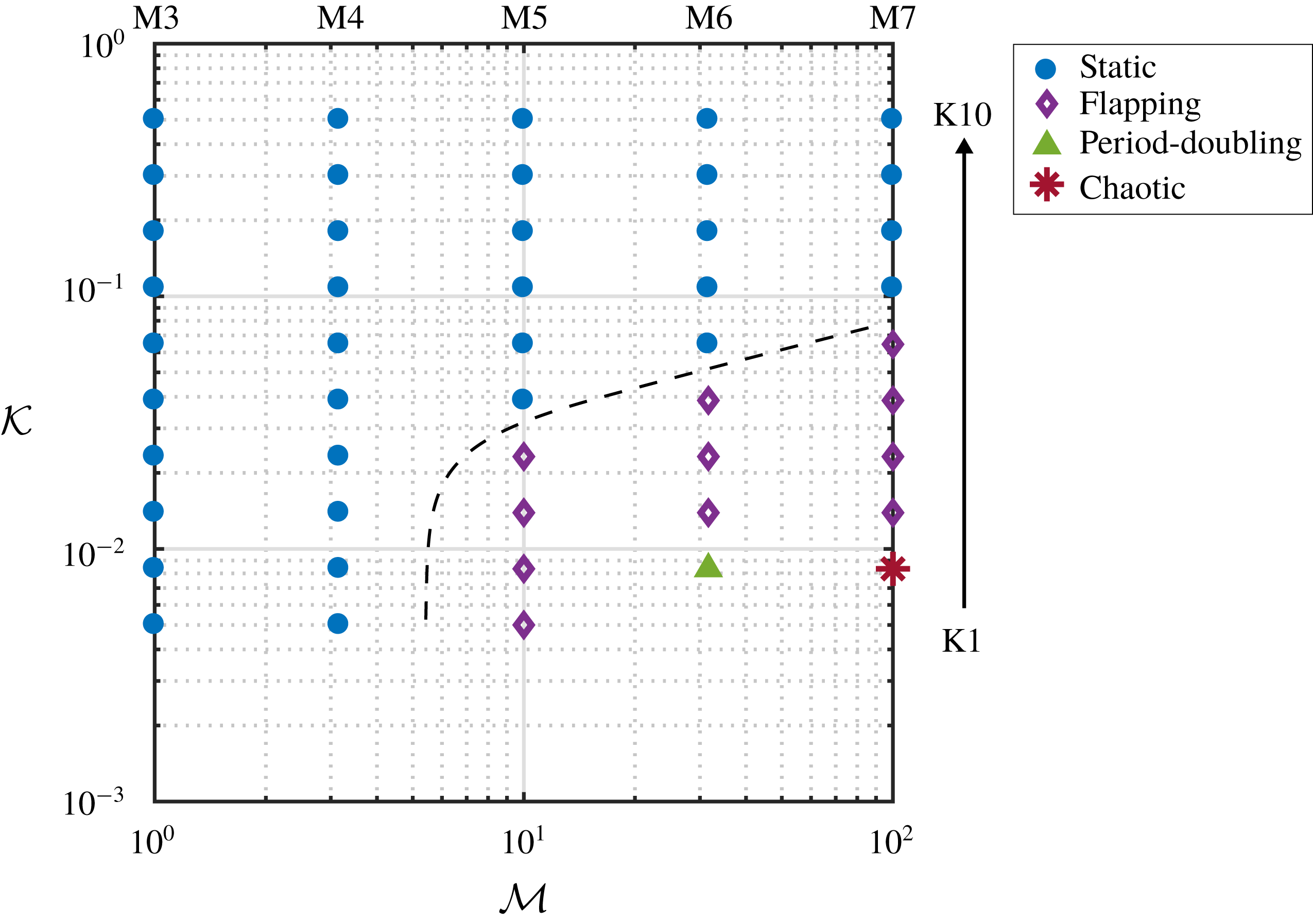
Figure 9 shows dynamic states over only a small region of the parameter space. However, it is still possible to make observations regarding the effect of the material properties. In particular, it is evident that the bending rigidity appears to be stabilising while mass ratio is destabilising. Although the literature regarding wall-mounted flaps in a steady cross-flow is somewhat limited (Lee et al. Reference Lee, Park, Kim, Ryu and Sung2017; Jin, Kim & Chamorro Reference Jin, Kim and Chamorro2018), Leclercq, Peake & de Langre (Reference Leclercq, Peake and de Langre2018) report similar effects concerning the mechanical properties of the flaps. Moreover, they also note that under large deformations the flap assumes a position resemblant of an axially aligned flag. This allows comparisons to be made with previous work on flapping flags and the literature surrounding this problem shows a similar trend with regards to the stabilising/destabilising effects of bending stiffness/mass ratio (Shelley, Vandenberghe & Zhang Reference Shelley, Vandenberghe and Zhang2005; Connell & Yue Reference Connell and Yue2007). It is expected that at larger mass ratios the window of dynamic motion would continue to increase in size. However, these were not tested here since the range of tested mass ratios (M3–M7) are already one order of magnitude larger than the tested mass ratios in the multiple flap case (M1–5). Furthermore, it is expected that the modelling challenges associated with the flap–wall contact would be exacerbated at larger mass ratios.
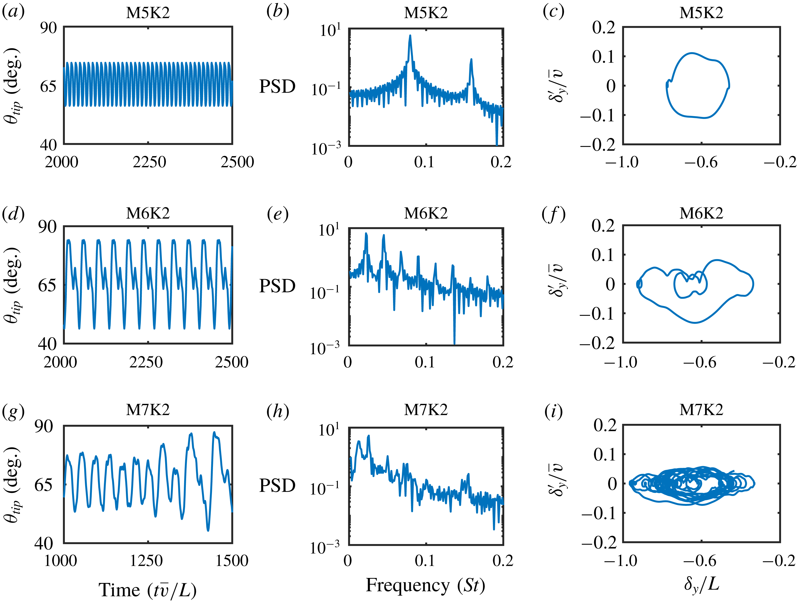
Tip angle histories, power spectra and phase plots of vertical tip motion for flapping (a–c), period doubling (d–f) and chaotic motion (g–i) for a single flap. The phase plots are taken over the same period of time as that shown in the tip angle histories.
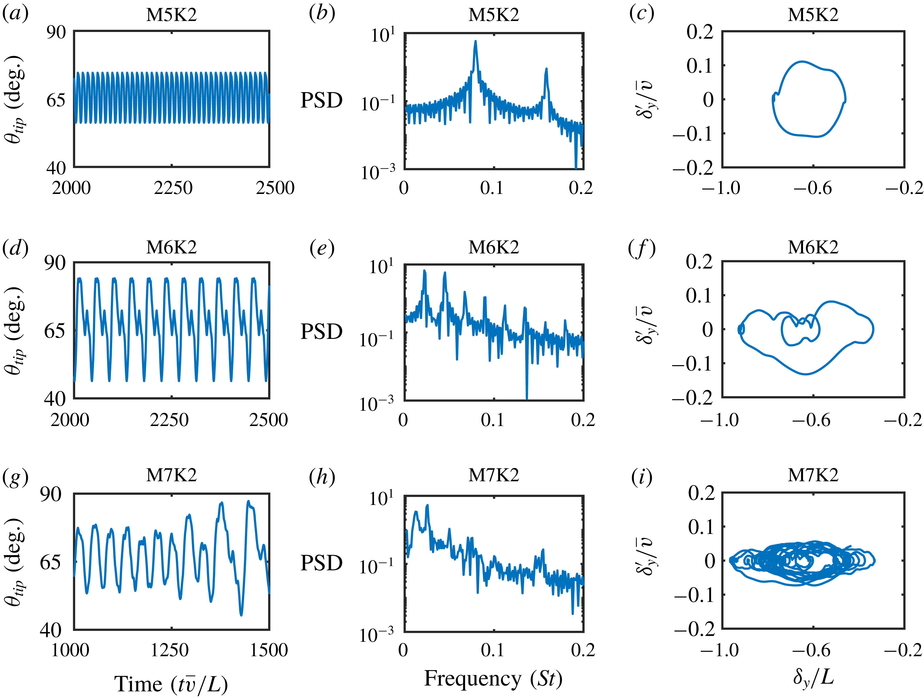
To help characterise the motion of the flap over the three dynamical states (flapping, period doubling, chaotic), figure 10 shows the tip angle histories and power spectra for each of these three states. Also shown are the phase plots, which depict the tip trajectories based on the vertical velocity (
 $\unicode[STIX]{x1D6FF}_{y}^{\prime }$
) and displacement (
 $\unicode[STIX]{x1D6FF}_{y}$
) of the tip. The chaotic case (M7K2) is plotted over a different time range, since soon after this the flap made contact with the bottom wall. The phase plots are taken over the same period of time as that given by the tip angle histories. For the flapping case (M5K2), the flap motion is seen to have a regular motion with constant amplitude and frequency. A small ‘kick’ in the tip motion is observable at the extremities of the flapping cycle, which is especially noticeable in the phase plot. At the next mass ratio (M6K2), a regular flapping motion is still observable. However, this now takes the form of a double-period cycle, with the secondary motion obtaining a significantly lower tip angle. Finally, at the largest mass ratio (M7K2) the tip motion and phase portrait describe a dominant low-frequency dynamic with superimposed high-frequency perturbations, indicating the onset of chaotic motion. This is supported by the power spectrum, which shows a wider distribution of power around the main frequency as well as secondary high-frequency peaks. It is worth noting that the transition from period one, to period two, then to chaotic motion would suggest a period-doubling cascade to chaos. Although, a finer resolution of the parameter space would be required to determine this.
5.2 Classification of states for array
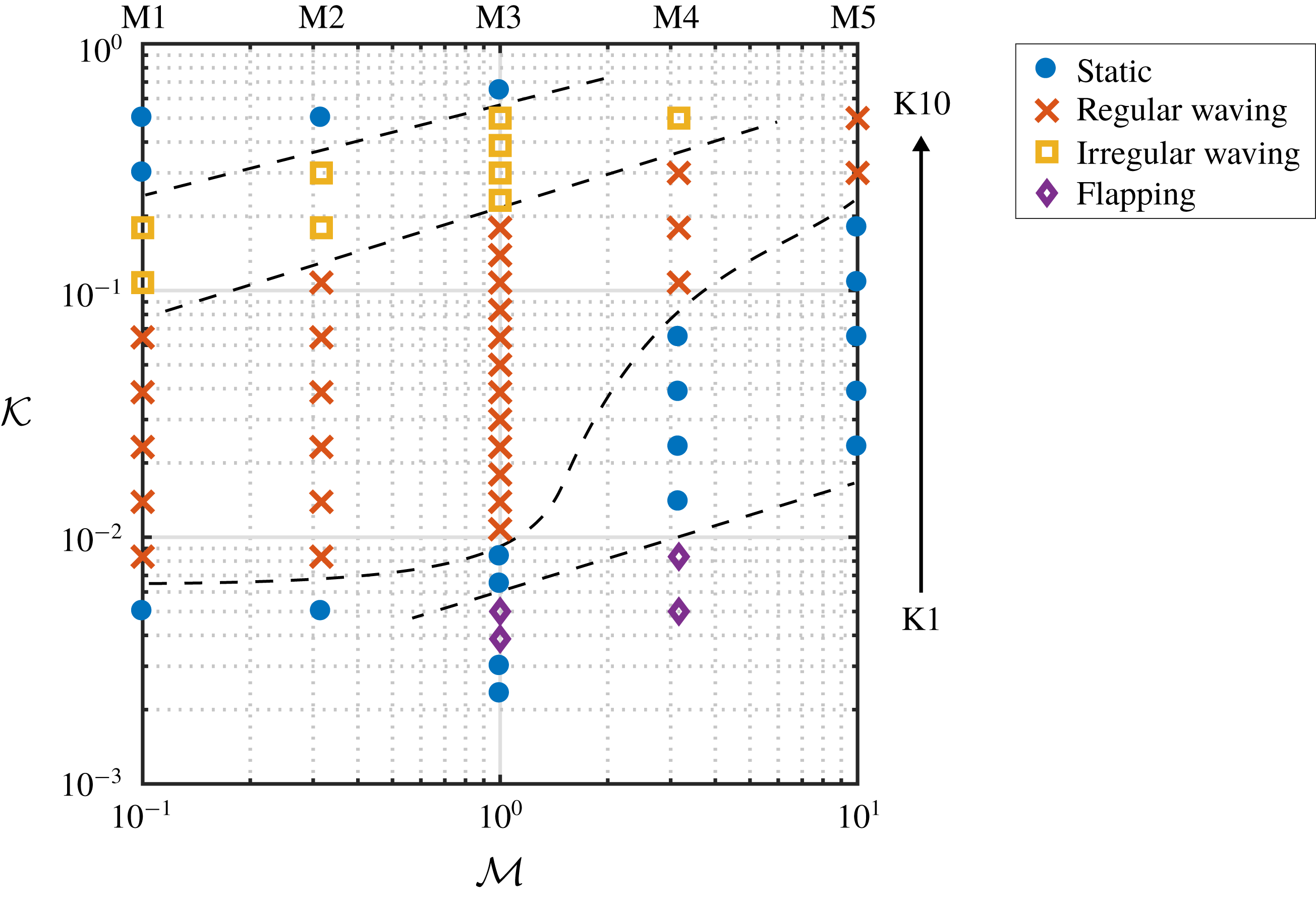
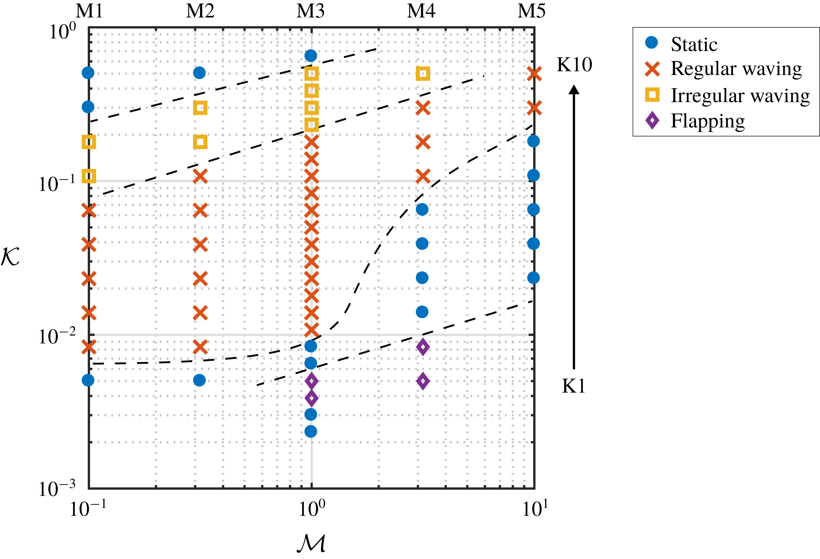
This section considers the case of 128 wall-mounted flexible flaps, as depicted in figure 6. Figure 11 shows the classification of the behavioural states for the array over the full parameter space (M1–5, K1–10). Subsequent to the initial parameter sweep, extra cases were run for the M3 branch and these are also shown in figure 11. Through a systematic process of analysis of the flap dynamics, each case is classified into one of four states: a static behaviour, a regular waving behaviour, an irregular waving behaviour, and a flapping behaviour. Note that cases where large mass ratios were combined with low bending stiffness (M5K1, M5K2, M5K3), contact between adjacent flaps led to stability problems and so results were not obtained for these cases. Examining the variation in behaviour with the structural properties of the flaps reveals a clear diagonally banded region of waving motion. Immediately adjacent to this are regions of static behaviour, which demonstrate the parametric sensitivity in this region. Meanwhile, the denoted static states themselves exhibit a broad range of tip deflection, depending on the bending stiffness. At large mass ratio/low bending stiffness, a region of flapping behaviour is observed. This flapping mode will be discussed in detail in § 5.3.
Parameter map with observed behaviour modes for array. Dashed line is shown to help distinguish boundaries. The range of mass ratio and bending stiffness is given by M1–5 and K1–10. Therefore, these mass ratios are shifted one order of magnitude lower compared to the single flap case. Note that extra cases were run for the M3 mass ratio, the results of which are discussed in § 5.5.
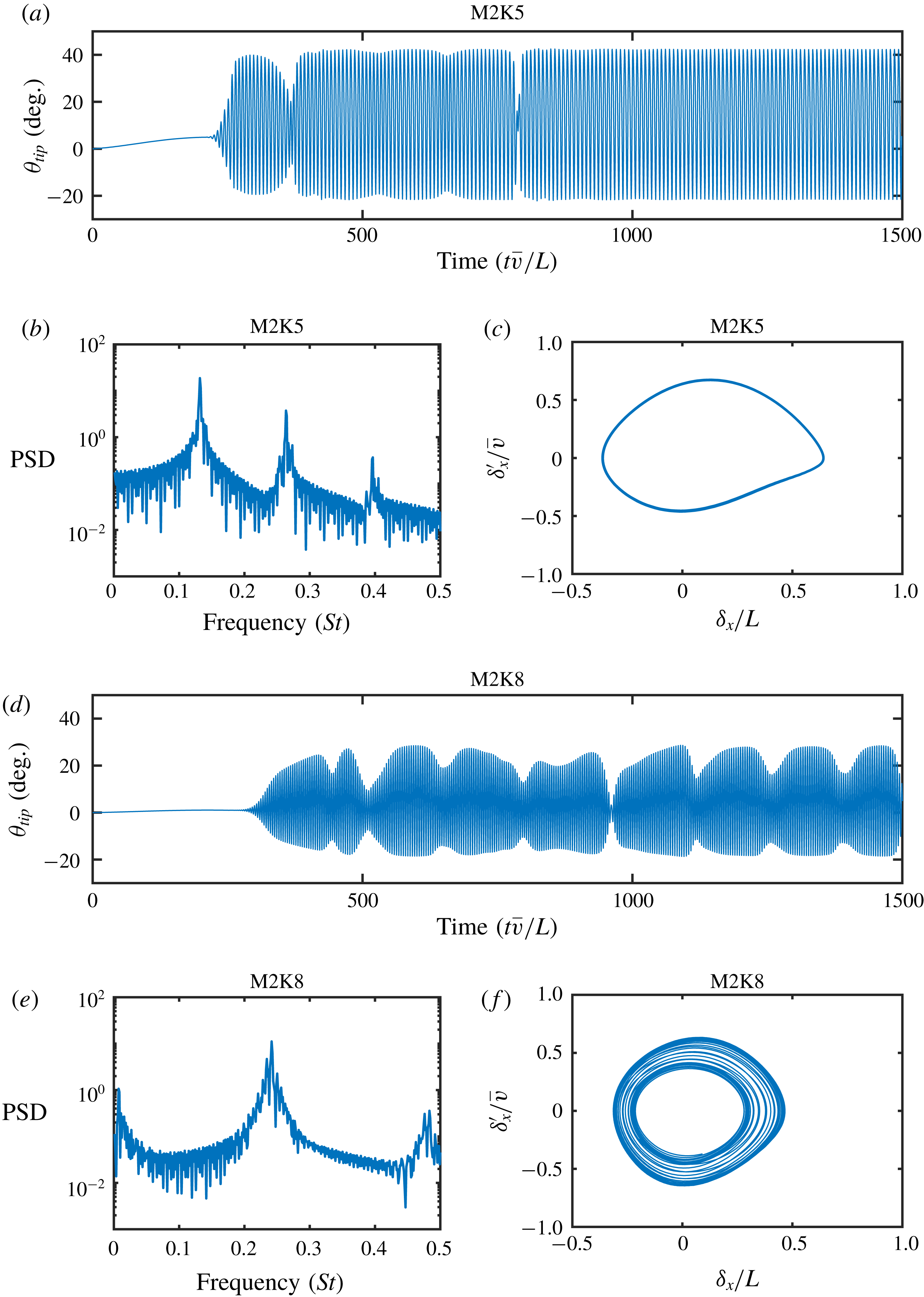
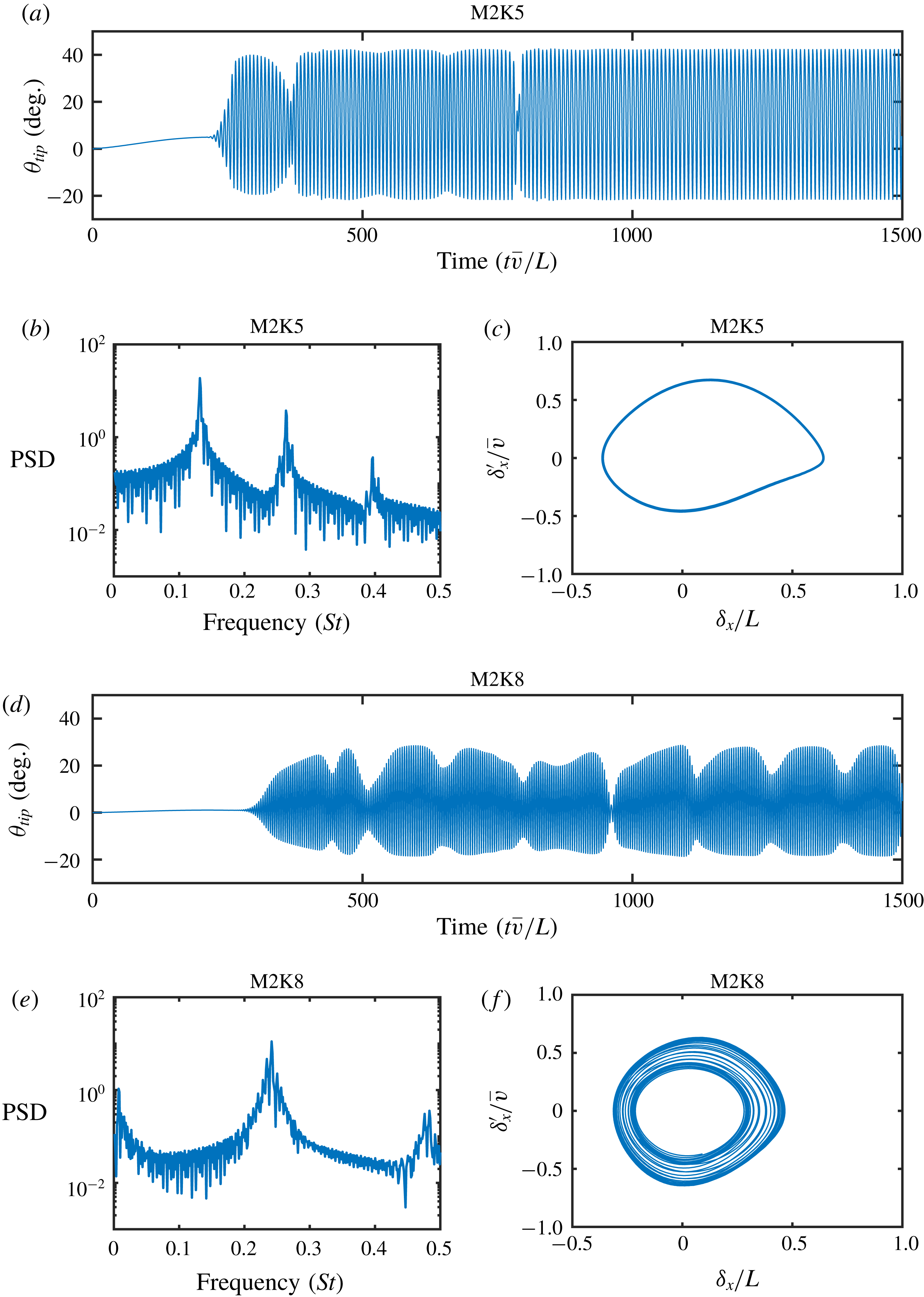
Tip angle histories, power spectra and phase plots of horizontal tip motion for regular waving (a–c) and irregular waving (d–f) for the 100th flap in the array. The phase plots are taken over the final 150 seconds of simulation, which corresponds to approximately 15 (regular waving) and 30 (irregular waving) periods of oscillation for these two cases.
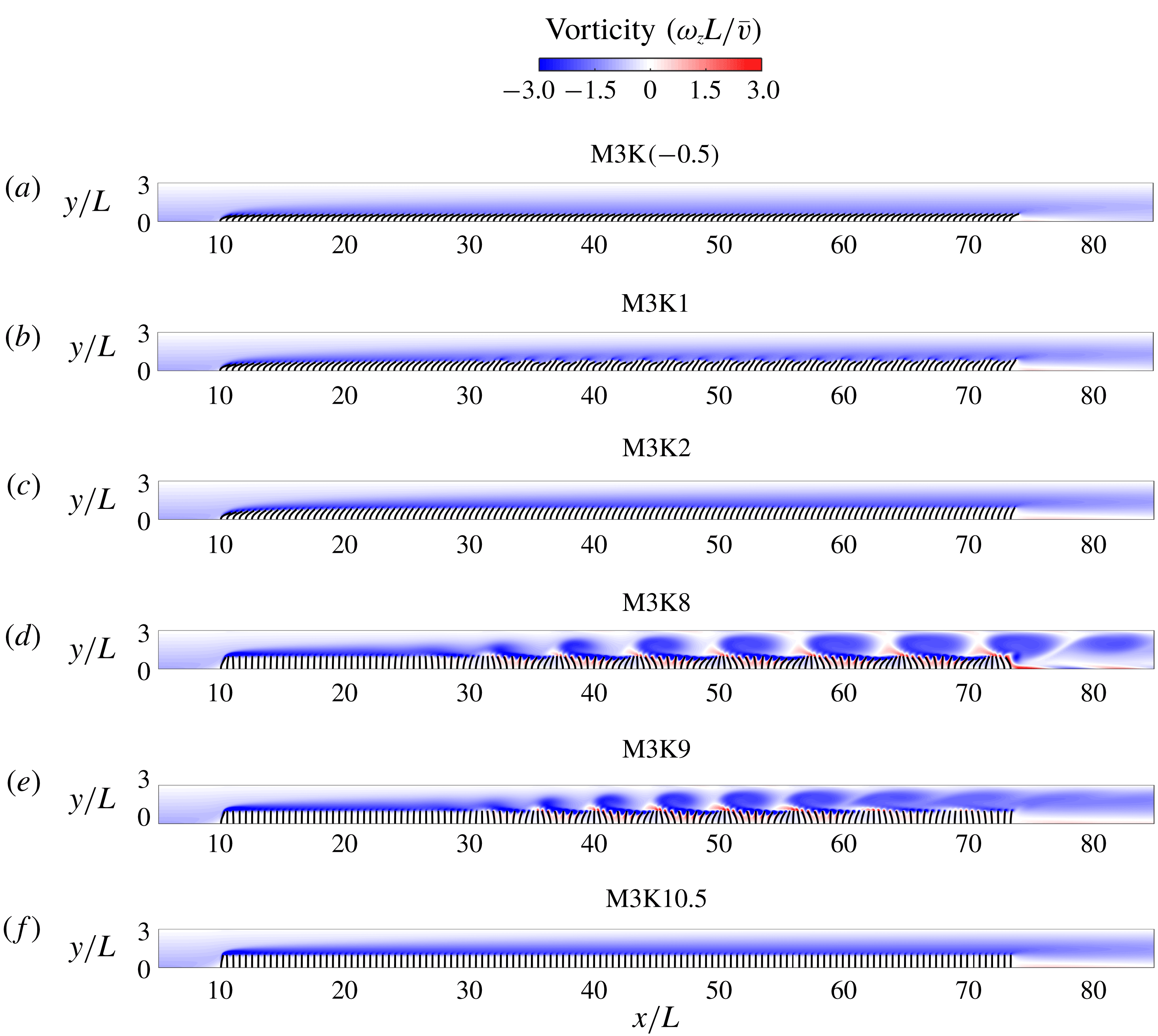
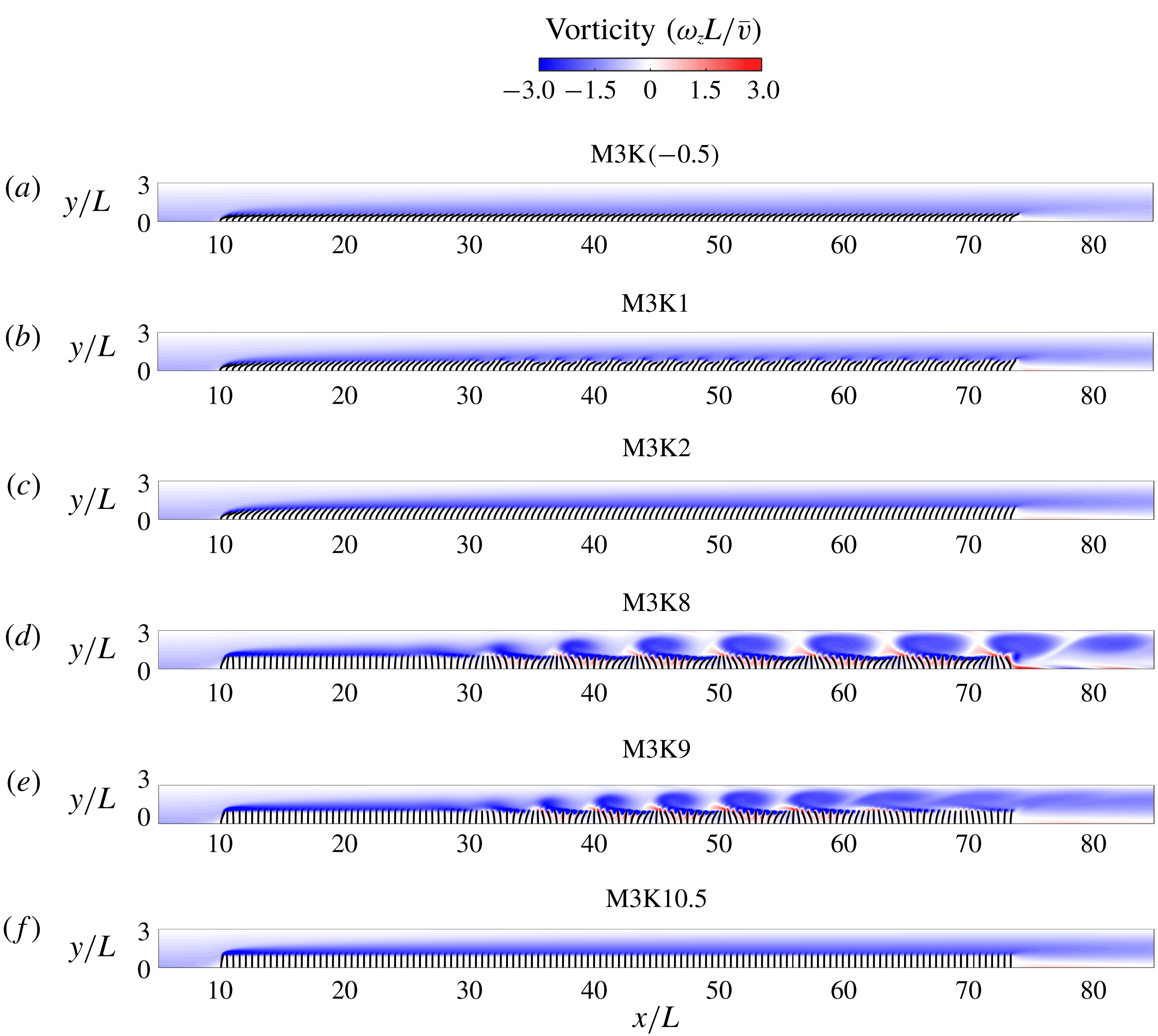
Snapshots of out-of-plane vorticity and flap positions across the whole array for six representative cases at the M3 mass ratio. (a) Static reconfiguration (large). (b) Flapping. (c) Static reconfiguration (moderate). (d) Regular waving. (e) Irregular waving. (f) Static with small deflection. Note that to capture the full range of observed states, the bending rigidities in (a) and (f) fall outside of the range originally defined in (4.4).
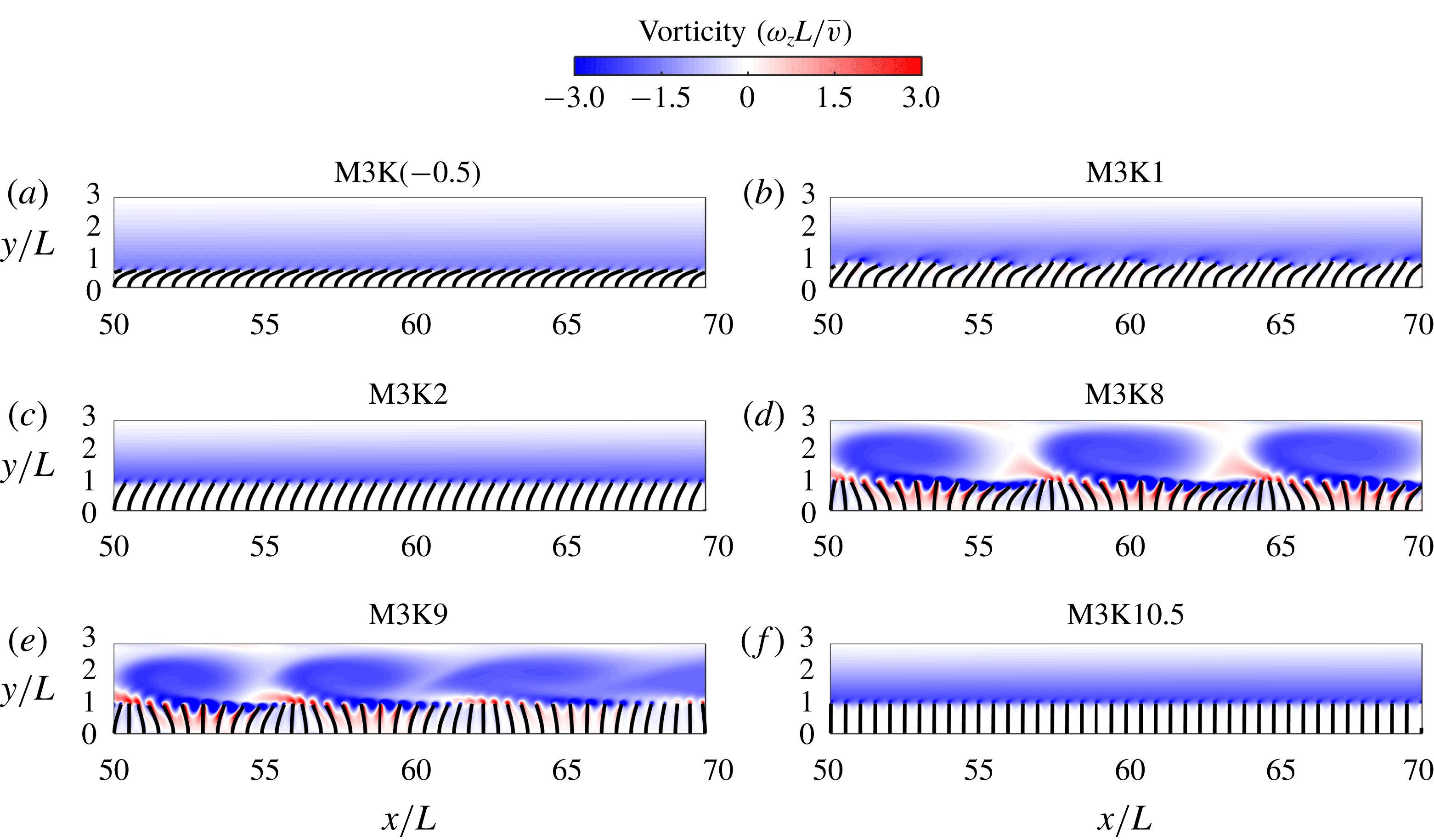
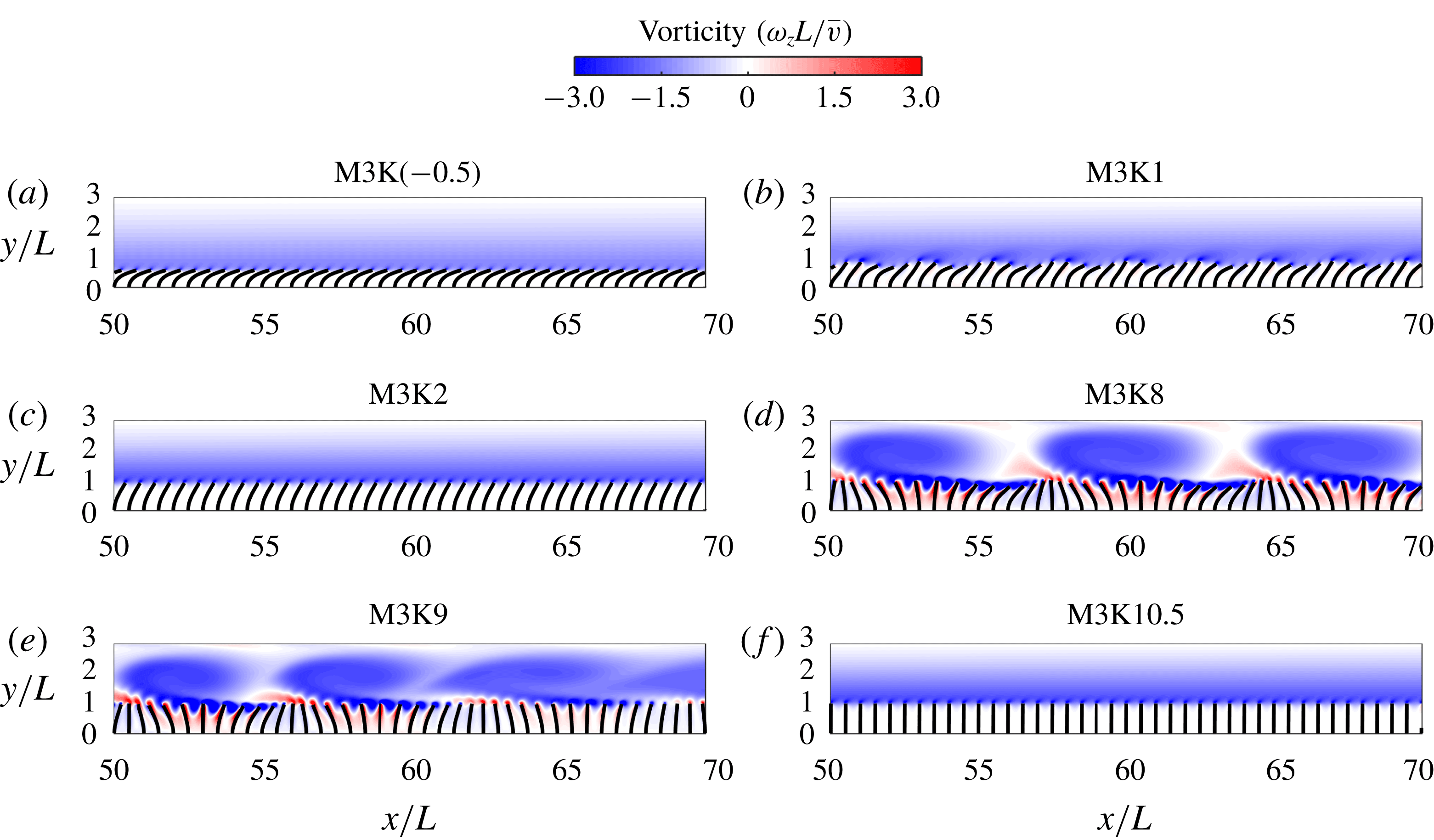
Enlarged snapshots of out-of-plane vorticity and flap positions across the whole array for six representative cases at the M3 mass ratio. (a) Static reconfiguration (large). (b) Flapping. (c) Static reconfiguration (moderate). (d) Regular waving. (e) Irregular waving. (f) Static with small deflection. Note that to capture the full range of observed states, the bending rigidities in (a) and (f) fall outside of the range originally defined in (4.4).
A distinction is made between the two types of waving motion: regular and irregular. Figure 12 gives an example of what is meant by this classification. Here, the tip angle histories, power spectra, and phase portraits of the streamwise tip deflection are shown for a representative flap along the channel. The 100th flap is chosen since the waving instability is fully developed at this point and all of the flaps within this region exhibit the same characteristic state. Furthermore, it is sufficiently far from end effects associated with the finite size of the array. For the case of regular waving (M2K5), after the initial transient the motion of the flap settles into a regular periodic motion with constant amplitude and frequency, which corresponds to the passage of individual vortices over the flap. However, in the case of irregular waving (M2K8), as well as the main high-frequency mode, there is a secondary low-frequency dynamic. This causes large temporal and spatial variations in the waving amplitude. This is especially evident in the power spectrum, which, as well as showing a low-frequency peak, has a wider distribution of power around the high-frequency dynamic. The phase portrait also helps to distinguish between the regular and irregular waving. Here, the streamwise tip deflection has been plotted over a period of 150 seconds, which corresponds to approximately 15 and 30 periods of oscillation for these two cases, respectively.
Figures 13–14 show snapshots of the flow field and flap deflection for six representative cases. For the first case (low bending stiffness), the behaviour is observed to be static with a drag-reducing reconfiguration. No instabilities are observed in the flow field or flap dynamics. However, as the bending stiffness is increased, the flapping mode emerges and instabilities start to develop approximately a third of the way along the channel. This instability is associated with small scale flow structures and a structural deformation representative of a mode-two deformation. Further increasing the bending stiffness leads to another region of static behaviour, this time with reduced deflection, before the appearance of the waving mode (regular and irregular). Like the flapping mode, the waving mode instabilities start to develop approximately a third of the way along the channel, but this time they roll up to form large coherent vortical structures. The appearance and behaviour of this instability depends heavily on the structural properties. In the case of the regular waving mode, after an initial development length the vortical structures eventually establish a fixed size. However, in the case of the irregular waving mode, the vortices are seen to break up with both spatial and temporal variation, which leads to the irregular flap dynamics. As the bending stiffness is increased further, the instabilities are suppressed and the behaviour becomes static again, this time with small deflection.
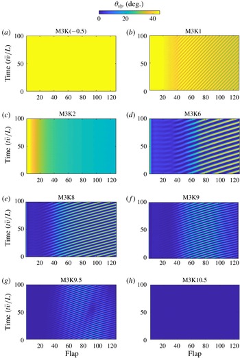
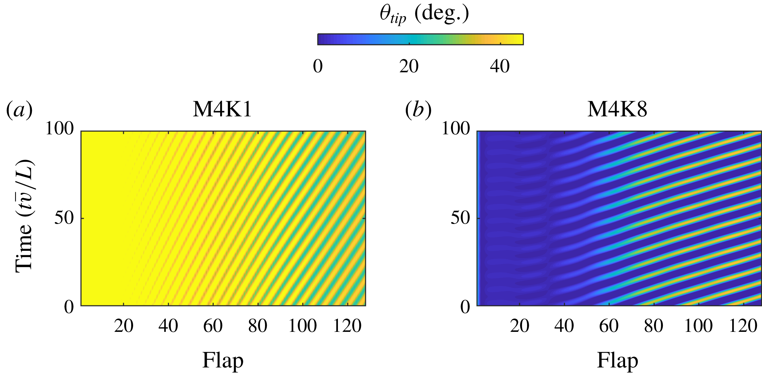
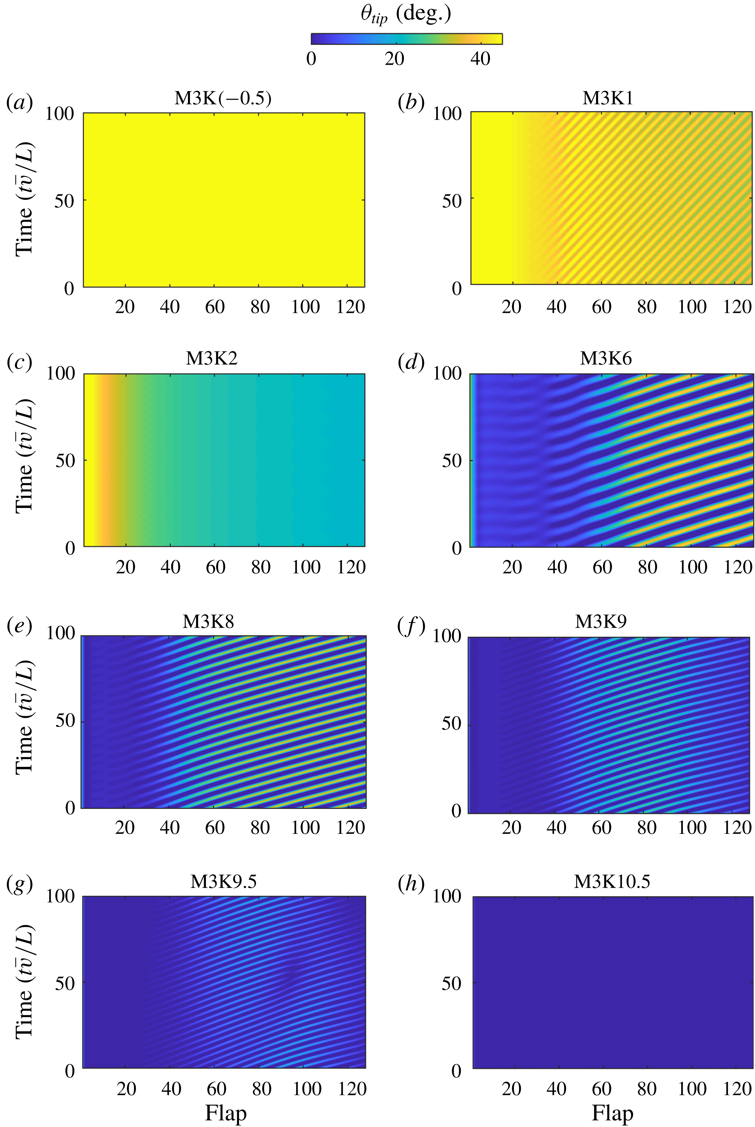
Contours of tip angle across the array over the final 100 seconds of simulation. To visualise the range of motion for each case the values beyond the colour scale have been clipped.
Four of the states reported in figures 13–14 are emblematic of the four characteristic regimes exhibited by aquatic vegetation, as described in Nepf & Vivoni (Reference Nepf and Vivoni2000). In order of decreasing flow speed, these states are usually described as prone (static reconfiguration), strong coherent swaying (regular waving), gentle swaying (irregular waving) and erect (static with small deflection). While these states are described in terms of flow speed, since the dimensionless bending stiffness is inversely dependent on flow speed (4.2), the trends observed in figures 13–14 are in line with those in the literature. However, in the context of this trend it appears that the flapping mode described in this work has not been previously reported in the literature.
Examining both the temporal and spatial patterns in the coupled dynamics is a challenging task. Figure 15 provides a convenient method for examining such patterns. For each flap along the array the instantaneous tip angle is plotted with time. This facilitates observations of a range of properties describing the system behaviour, including the development length, wavelength, frequency and wave speed of the instabilities, as well as the global behaviour mode. Clearly visible is the effect of bending stiffness and the resulting transition from static reconfiguration, through the flapping and regular waving modes (with increasing frequency of motion), until a breakup of the spatial and temporal coherence through the array occurs at large bending rigidity (irregular waving mode). Also noticeable is a narrowing of the ‘waving bands’ as the bending rigidity is increased, which corresponds to an increase in the frequency of motion.
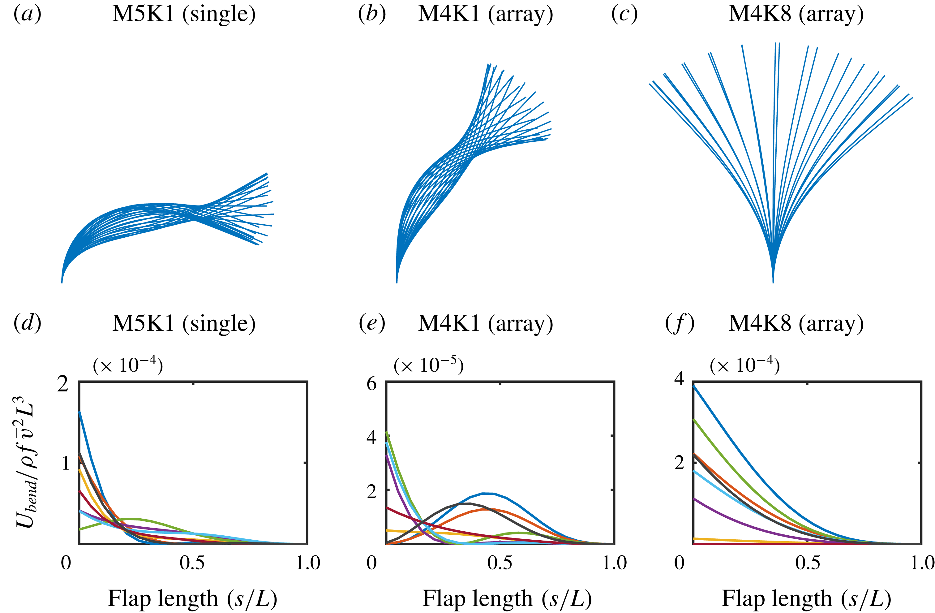
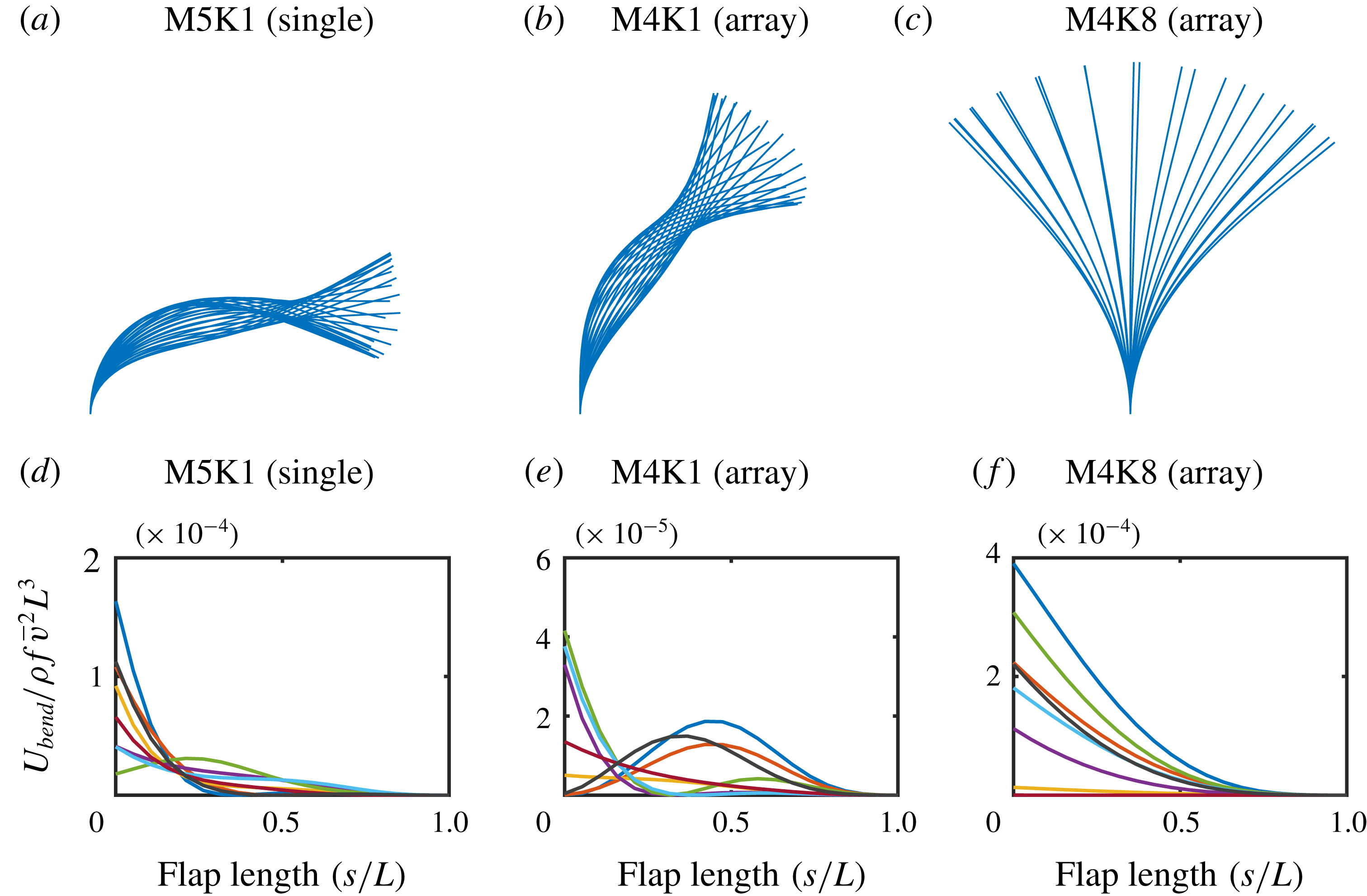
Flap profile shapes and bending strain energy along the length of the flap for flapping and (regular) waving modes. The strain energy distributions are extracted at eight equally spaced snapshots within a single period of motion. (a,d) Single flap in flapping mode. (b,e) Array in flapping mode. (c,f) Array in waving mode. For the array cases the 100th flap is shown.
5.3 Flapping state
Figures 13(b) and 14(b) display the contours of the out-of-plane vorticity and flap positions for the flapping mode. A series of smaller scale flow structures are visible, which span a smaller number of flaps compared to the waving mode. Furthermore, examination of the flap positions indicates a different deformation mode to that observed in the waving cases.
Figure 16 shows snapshots of a representative flap profile over one cycle for both the (regular) waving and flapping modes. For comparison, the flapping mode observed for a single flap is also shown. This figure clearly distinguishes the flapping mode from the waving mode in the array behaviour. Both the single flap and the flapping state in the array exhibit a clear necking behaviour in the profile snapshots. This is evidence of the mode-two deformation that is associated with flapping motion. Although the bending rigidity for these two cases is the same, the single flap shows a greater degree of deflection. This can be attributed to the presence of the adjacent flaps in the array, which act to impede the motion. Also noticeable is the fact that the waving motion is dominated by mode-one deformation. As will be shown in § 5.4, the emergence of the flapping motion is a result of the mode-two natural frequency approaching the estimated natural frequency of the mixing layer instability.
Figure 16 also shows the distribution of strain energy due to bending (
 $U_{bend}$
) within the flap, where
 $s$
is a parametric coordinate along the flap length. The strain energy distributions are extracted at eight equally spaced time intervals within a single period of motion. In the case of the (regular) waving state, the location of maximum strain energy always occurs at the base of the flap and the strain energy decreases exponentially towards zero at the flap tip. However, in the flapping cases there are instances within the cycle where the maximum strain energy occurs away from the base towards the middle of the flap. This is less prominent in the case of the single flap, since the large deformations experienced at the base of the flap lead to increased strain energy levels in this region, which partially obscure the distributions along the rest of the flap. Nevertheless, these findings are indicative of mode-two dynamics and further support the classification of the flapping state.
Contours of tip angle across the array over the final 100 seconds of simulation for the flapping (a) and regular waving (b) modes. To visualise the range of motion for each case the values beyond the colour scale have been clipped.
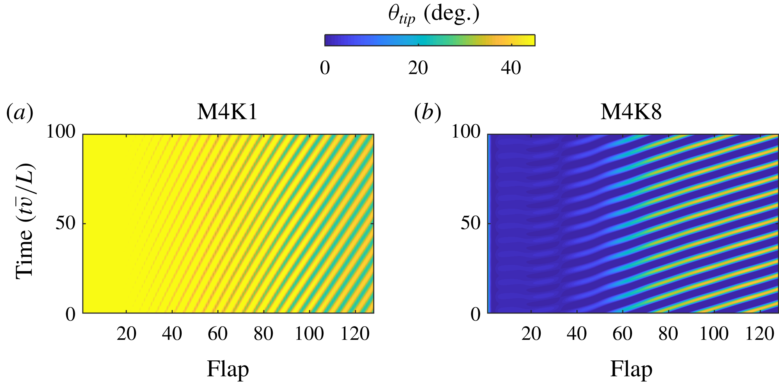
Figure 17 compares the spatial and temporal variations in tip angle for the flapping and regular waving modes. The flapping mode is characterised by a larger mean value for the tip angle but a smaller amplitude of motion, when compared to the regular waving mode. Further observations regarding the frequency and wave speed can be made by examining the size of the waving bands. The vertical distance between the bands infers the period of the motion, whereas the angle (measured with respect to the time axis) of the travelling bands gives the wave speed. While both of these cases exhibit similar frequencies, the wave speed is dramatically different, with a much lower wave speed observed for the flapping case. Since the wavelength is related to the frequency and wave speed, this implies the size of the flow structures are significantly smaller for the flapping case. This observation is supported by examining the vorticity contours in figure 14(b).
5.4 Frequency of instability
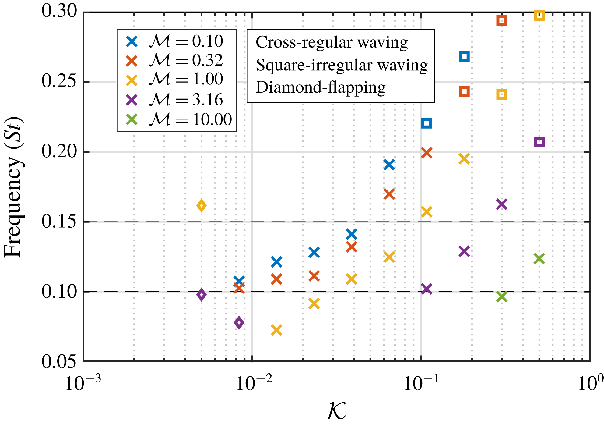
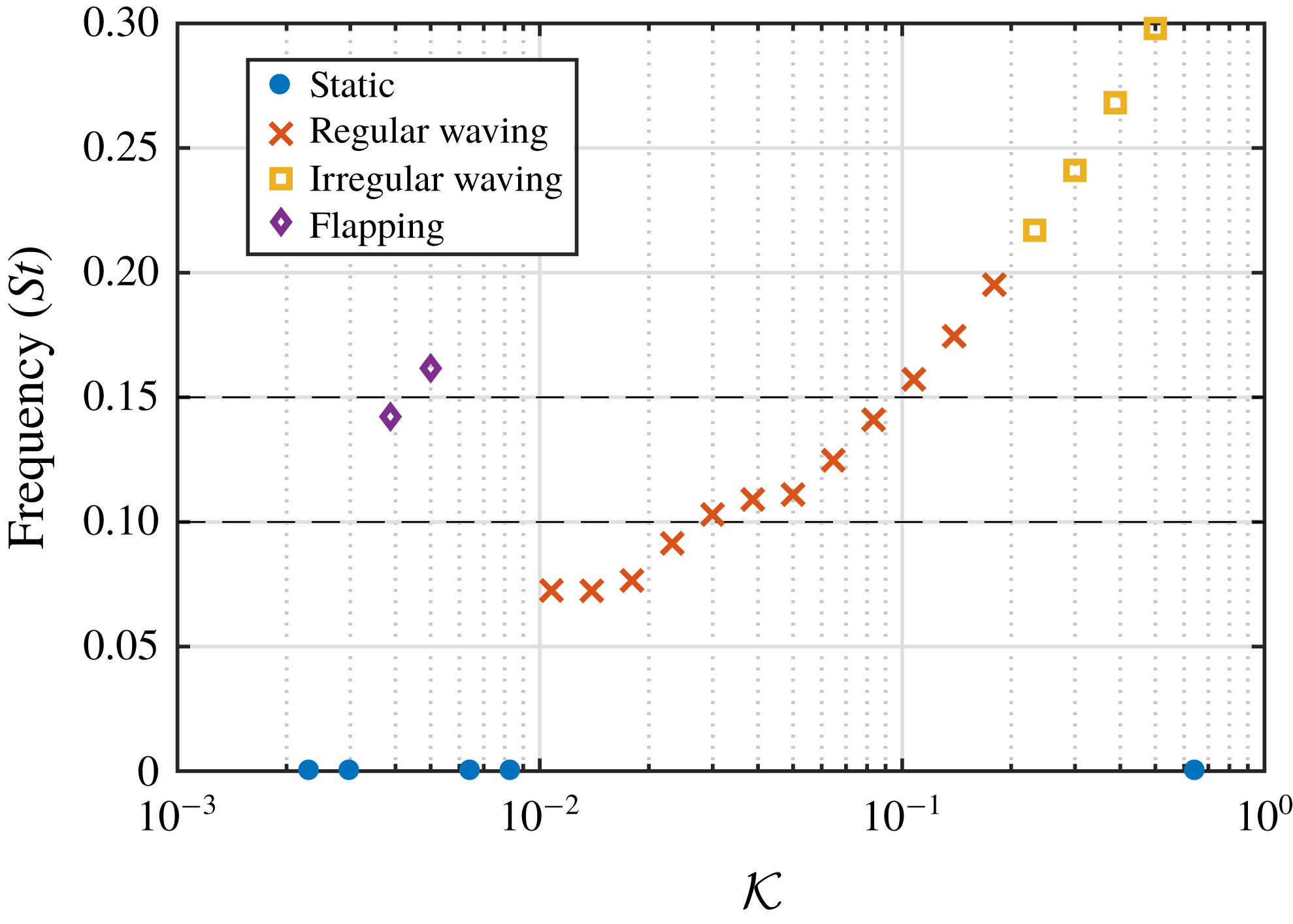
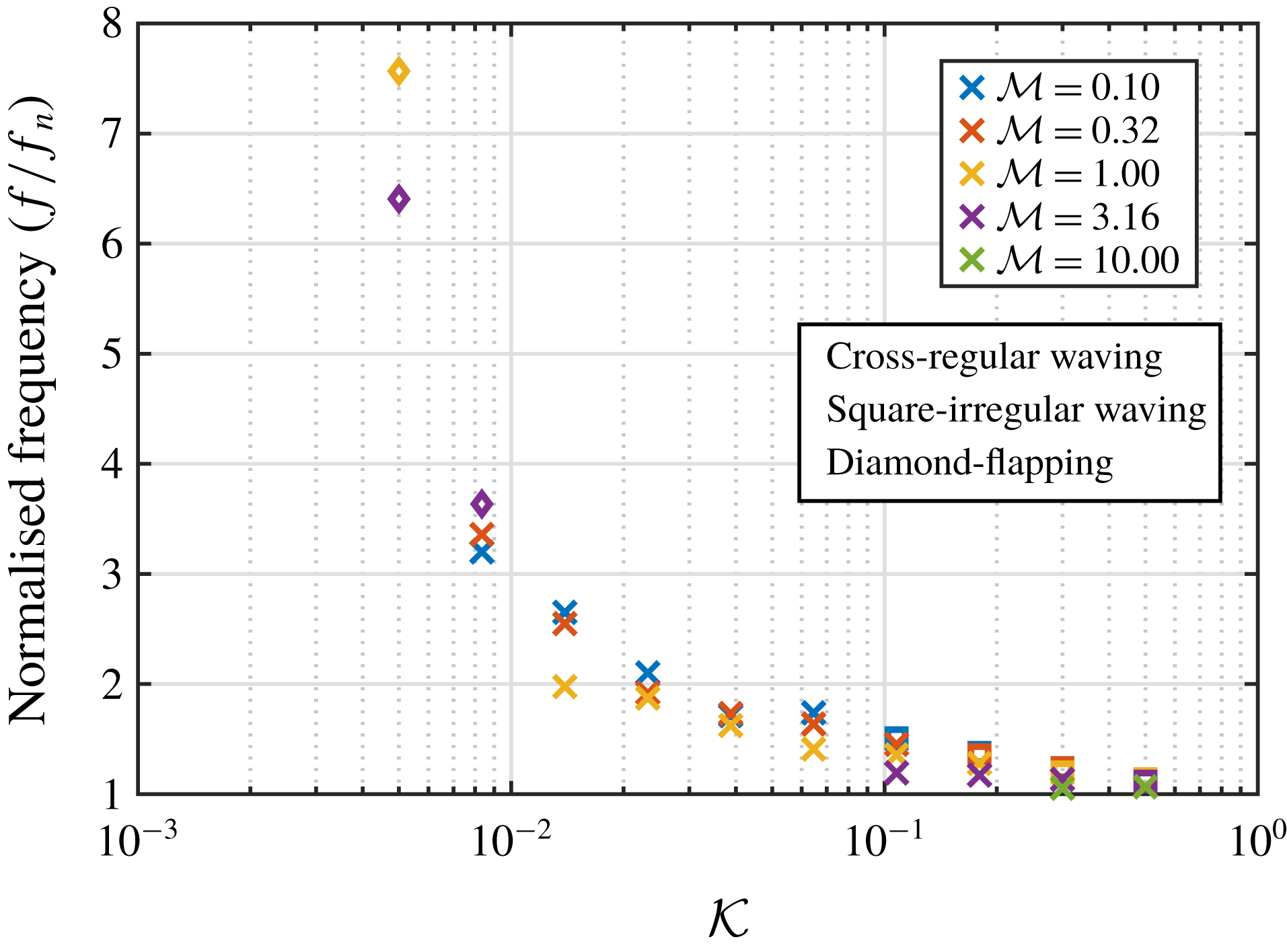
Figure 18 shows the mean frequency of motion across the whole array for each dynamic case. Several key observations can be made regarding this figure. First, there is a large variation in frequency over the tested parameter space. This indicates that there is indeed a coupled dependence of the waving instability on the structural properties of the array. Furthermore, the regular waving mode seems to largely exist within a well-defined frequency range (
 $St=0.1{-}0.2$
). To estimate the frequency of the mixing layer instability, a rigid configuration was tested and the steady-state velocity profile extracted. Using (1.1), the frequency of the mixing layer instability for this set of flow conditions was found to be approximately
 $St_{KH}=0.13$
. This falls within the range of the regular waving frequencies and suggests that the governing mechanism for the dynamic motion is a coupling of the mixing layer and structural natural frequencies. This may also explain the transition to the irregular waving state, where the imbalance between the two frequencies leads to a competing behaviour between the fluid and structure. For a sample of selected flexible cases the time-averaged velocity field for the dynamic cases was also used to estimate the mixing layer frequency. The range of predicted values was found to be 0.1 to 0.15, which is within the observed range of regular waving frequencies and thus further supports this finding.
Mean frequency of motion across the whole array for each case that exhibited dynamic interactions. Marker shapes correspond to the states observed in figure 11. Dashed lines show range of estimated natural frequency of the mixing layer (Kelvin–Helmholtz) instability.
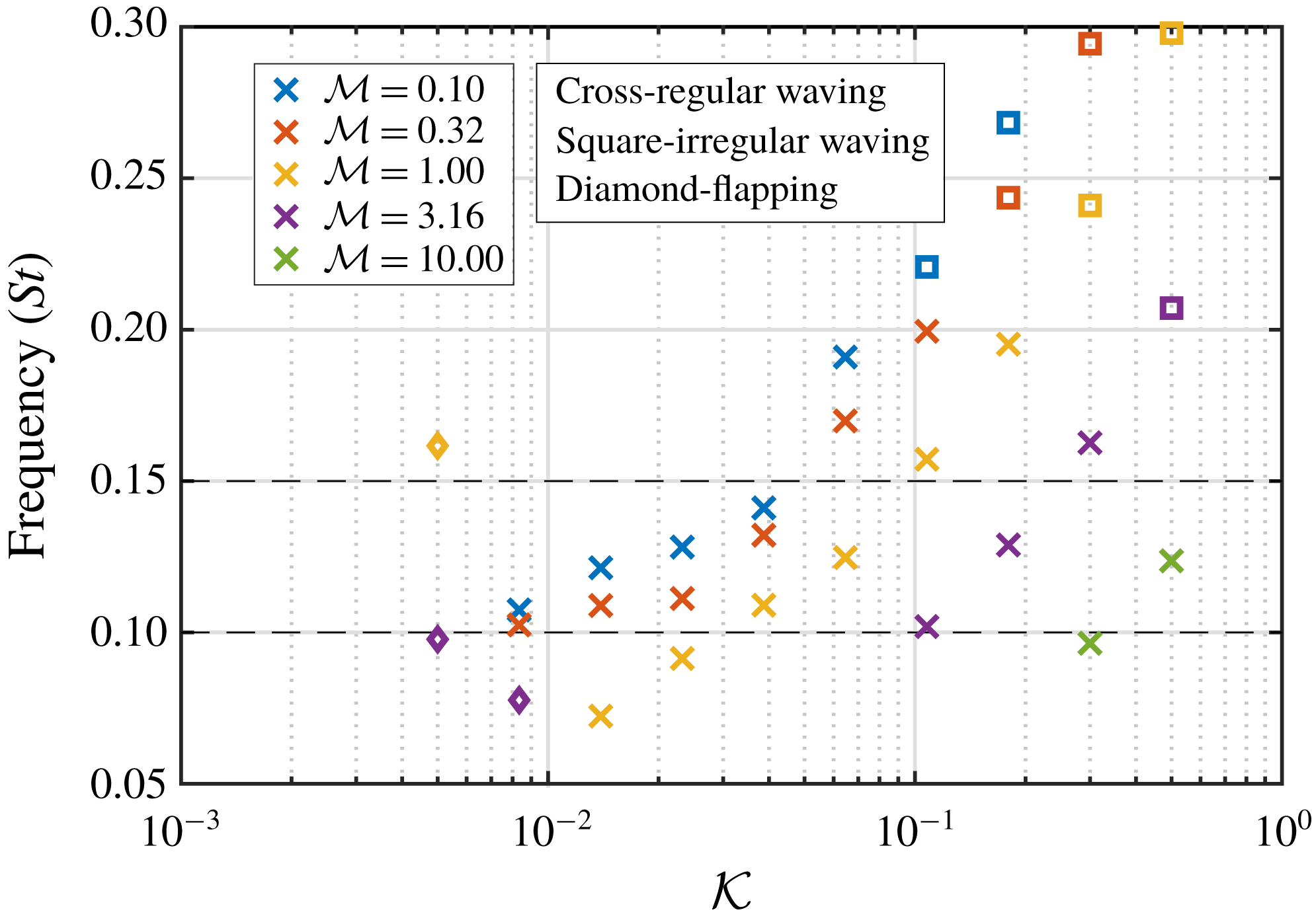
The waving cases observed in figure 18 indicate a monotonic relationship between the bending rigidity and frequency; the latter decreasing with the former. However, the three cases displaying a flapping motion are shown to deviate from this trend. Instead, for these cases there is a jump in the frequency as the behaviour transitions from waving to flapping. This can be explained by the fact that the main deformation mode for the flapping state is the second mode, which is associated with higher-frequency motion. In particular, the emergence of the flapping state seems to correspond to the point where the bending rigidity is sufficiently reduced to enable the mixing layer instability to excite the second mode, rather than the first mode. Since the waving motion is governed by mode-one deformation, this jump in frequency between the waving and flapping states is intuitive.
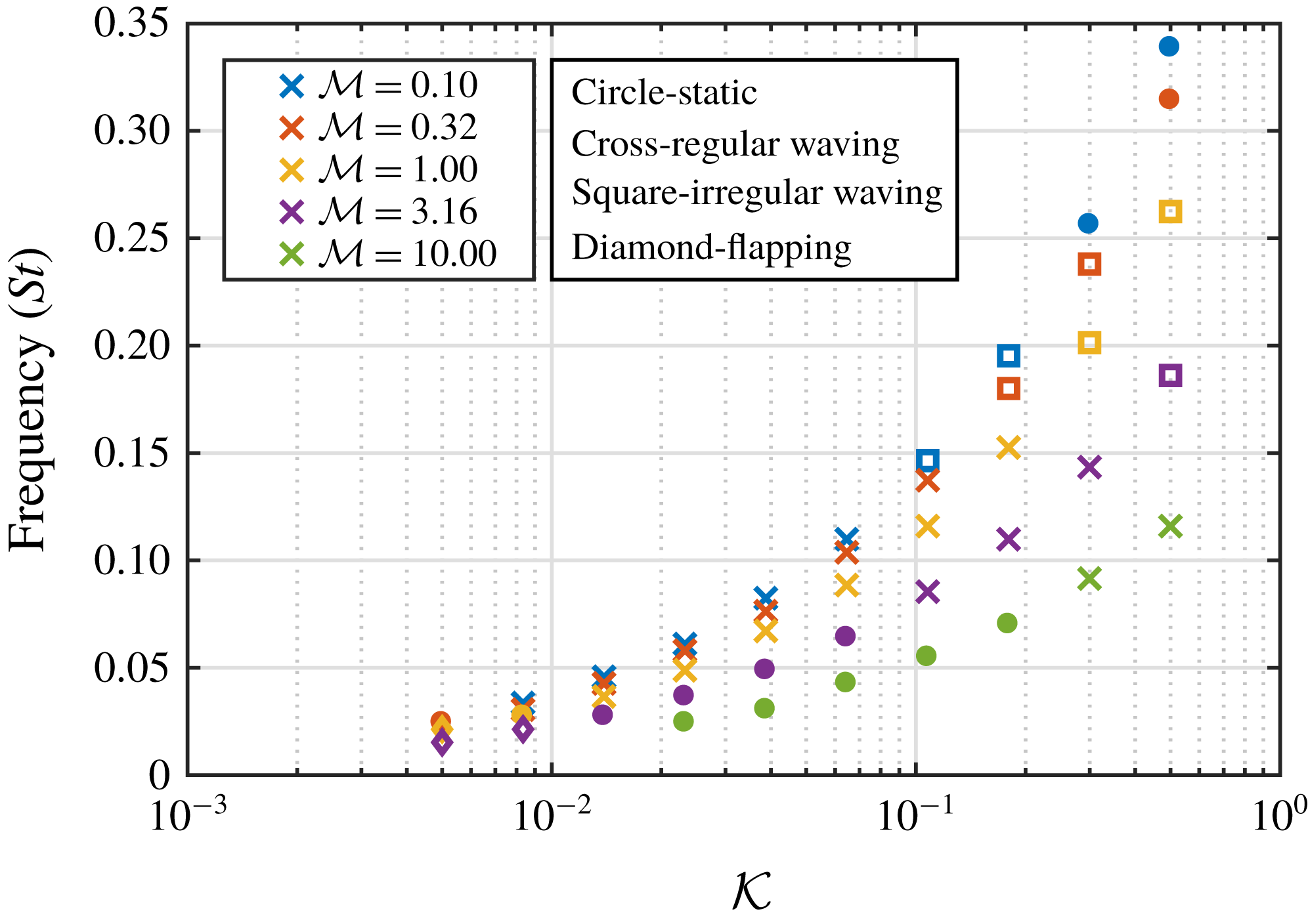
The results in figure 18 clearly demonstrate the dependency of the waving frequency on the structural natural frequency, with increasing frequency observed for low-mass/high-stiffness cases. To examine this relationship, a series of additional simulations were performed to numerically obtain the damped natural frequency of the array, by performing a free-oscillation test in a stagnant fluid. This was realised by removing the cross-flow and initialising the flaps with a horizontal tip deflection of
 $0.5L$
(while ensuring the correct initial stress field). At the start of the simulation the flaps were released and left to oscillate freely and the natural frequency of the array as a whole was measured. The results from this test are shown in figure 19. The markers in the figure indicate the states observed from the corresponding results reported in figure 18, and for completeness the natural frequencies of the cases that presented as static in figure 11 are also shown. As expected, the structural mass has the effect of decreasing the natural frequency, whereas the bending rigidity has the effect of increasing it.
Natural frequency of the array in a stagnant fluid, as measured in the free-oscillation test. Note that the marker shapes are based on the states observed in figure 11, not the free-oscillation test.
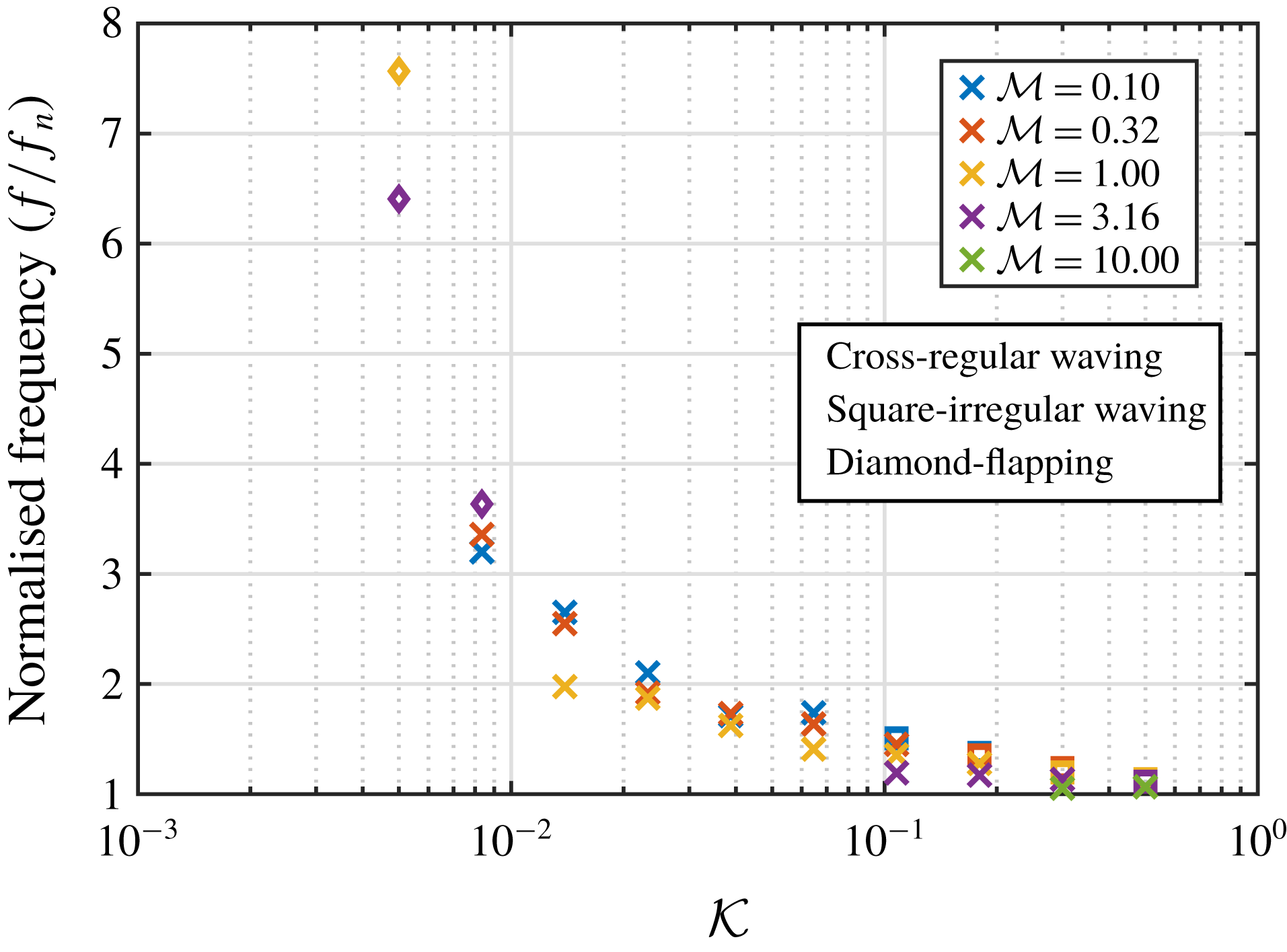
Normalised mean frequency (
 $f/f_{n}$
) of motion across the whole array for each case that exhibited dynamic interactions. Marker shapes correspond to the states observed in figure 11.
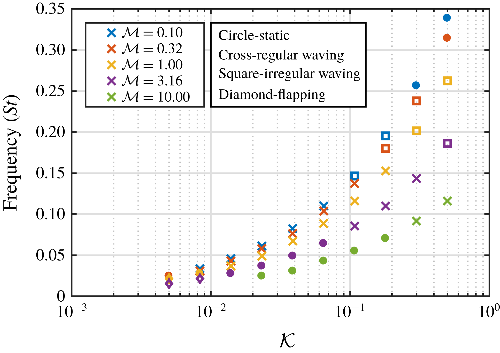
Mean frequency of motion across the whole array for the full range of M3 mass ratio tests. Marker shapes correspond to the states observed in figure 11. Dashed lines show range of estimated natural frequency of the mixing layer (Kelvin–Helmholtz) instability.
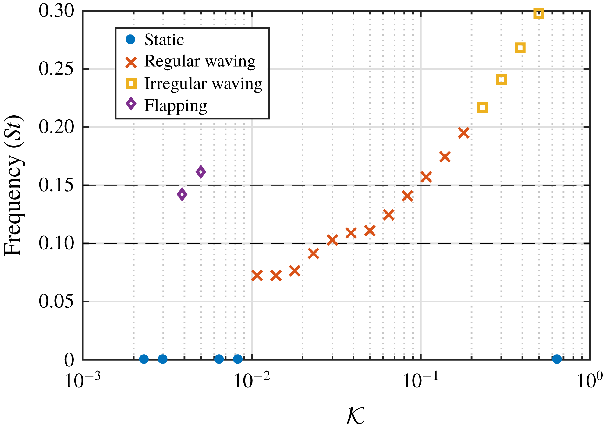
Figure 20 displays the measured frequencies from the cross-flow cases (figure 18) normalised by the natural frequencies from the free-oscillation tests (figure 19). It should be noted that the apparent trend reversal in measured frequency is due to the fact that each point in figure 20 has been normalised by its own unique natural frequency. The normalisation collapses the data across mass ratios onto a single curve. It is clear to see that a large number of cases exhibit dynamic motion at a frequency that is in the region of the natural frequency of the array. Furthermore, this ratio approaches unity as the bending stiffness increases. This is likely due to the increased bending energy stored in the flaps, which results in the natural response of the structure dominating the motion. Also noteworthy is the large disparity between the natural frequency and the observed frequency for the flapping cases, which is perhaps unsurprising since the free-oscillation tests were set up to measure the first natural frequency of the flaps, as opposed to the second mode which dominates the flapping motion.
5.5 Transition between states
To further investigate the transition over the full range of behaviours, extra cases were run for the M3 mass ratio, as shown in figure 11. The resulting states and frequencies from this analysis are shown in figure 21. The full range of observed behaviours are exhibited in this figure; starting from static behaviour at low bending rigidities, moving to the flapping mode with increasing bending rigidity, through another region of static behaviour, then through the regular and irregular waving modes, before finally becoming static again. Clearly observable is the jump in frequency between the flapping and waving modes. Furthermore, in the centre of the regular waving mode region there appears to be a plateau in frequency at approximately
 $St=0.11$
, which falls within the range of estimated frequencies for the mixing layer instability (
 $St_{KH}=0.1{-}0.15$
). A similar plateauing region has been reported in previous studies (Py et al.
Reference Py, de Langre and Moulia2006; Gosselin & de Langre Reference Gosselin and de Langre2009) where, as the natural frequencies of the mixing layer instability and canopy approach each other, the frequency response of the coupled system deviates from its observed trend and locks on to the synchronised natural frequencies of the mixing layer and canopy. This lock-in response is resistant to small but finite perturbations of the material properties around this state (
 ${\mathcal{K}}=0.03{-}0.05$
), as evidenced by the change in gradient of the frequency response in this region. This further supports the claim that the regular waving mode is triggered by a lock-in effect, whereas the other modes are associated with asynchronous natural frequencies between the fluid and the array. Examining the M1 and M2 branches in figure 18 shows similar indicators of lock-in within this region. However, more data points are required to ascertain whether or not the M4 and M5 branches also exhibit this behaviour.
6 Conclusions
To investigate the coupled interactions between fluid flows and arrays of slender structures, a large array consisting of 128 wall-mounted flexible flaps in an open-channel flow has been studied via numerical simulation. The flaps were modelled directly, so that local effects and interactions were captured. In particular, the coherent waving interactions (honami/monami), and the mechanisms that drive this instability, have been characterised over a range of mass ratio and bending rigidity.
The results show a broad range of behaviours over the tested structural properties. The coherent waving interactions (regular waving mode) were found to occur when the damped natural frequency of the array approached the predicted frequency of the mixing layer instability. Furthermore, this regular waving motion was shown to be linked to a lock-in between the natural frequencies of the fluid and structure. For a fixed mass ratio (M3) in the regular waving regime, the frequency response of the coupled system deviated from its observed trend and locked on to the synchronised natural frequencies of the mixing layer and canopy. This manifested as a plateauing of the frequency response within this region of the parameter space. A similar plateauing region was also observed for other mass ratios (M1 and M2). However, further tests are required to ascertain whether this effect is universal across the entire parameter space.
Different behavioural states emerged for cases where there was a disparity between the natural frequency of the array and the predicted frequency of the mixing layer instability. For an increase in the array natural frequency, the regular waving mode transitioned to an irregular waving state, characterised by large spatial and temporal variations in the structural response, before eventually transitioning to a static state with small deflection. For a decrease in natural frequency, the regular waving mode initially transitioned into a static state with moderate deflection. Further decreasing the natural frequency led to a regime where the mixing layer frequency excited the second structural mode. The observed behaviour in this regime was found to be similar to the flapping behaviour exhibited by single flaps, and is characterised by small scale flow structures. Finally, further decreasing the natural frequency eventually led to another static regime, this time with large deflection.
After examining the frequency of the flap motion and normalising with respect to the natural frequency of the array, the system response across the examined parameter space was shown to collapse onto a single curve. Furthermore, this ratio approached unity with increasing bending rigidity. These results suggest that the coherent waving motion commonly observed in vegetation is in fact a coupled response between the fluid and the array, as opposed to a purely fluid-driven instability. Moreover, the observations described here have important implications for flow control, where similar waving motions and lock-in effects have been observed, and demonstrate the potential for tuning coupled behaviour by modifying the ratio between the natural frequencies of the fluid and structure.
As discussed in the introduction, a significant limitation of the present work is the restriction to two dimensions. The primary effect of this restriction is to increase the blockage effect of the canopy, and therefore the drag imparted by the canopy on the flow. In turn, this will modify the velocity profile and alter the location and intensity of the inflection point. Since the inflection point is the trigger for the Kelvin–Helmholtz instability, this is likely to have a significant effect on the behaviour of the initial instability and its subsequent development. However, since the focus of the present work is the interaction between the natural frequencies of the mixing layer instability and canopy, the conclusions described here are likely to be independent of the characteristics of the initial onset of instability. Furthermore, while the Kelvin–Helmholtz vortices in terrestrial and deeply submerged canopies are highly three-dimensional, due to interactions with the boundary layer turbulence, for shallow submerged canopies, like the configuration presented in this work, the coherent flow structures remain predominantly lateral to the canopy and two-dimensional in nature.
Due to the large parameter space associated with these systems, there are several possible avenues for future research. The effects of Reynolds number, flap spacing, and blockage ratio are all worth investigating. Furthermore, incorporating heterogeneity effects, such as spatial variations in flap length, spacing and material properties, would provide results more applicable to real-world applications and can be readily incorporated via the present modelling approach. Moreover, to test the robustness of the coupled instability and its associated lock-in, unsteady flow conditions, due to gusting or oscillating flow, should be tested over a range of frequencies.
Acknowledgements
The authors would like to acknowledge the use of the Computational Shared Facility at The University of Manchester and the ARCHER UK National Supercomputing Service. Support from the UK Engineering and Physical Sciences Research Council under the project ‘UK Consortium on Mesoscale Engineering Sciences (UKCOMES)’ (grant no. EP/L00030X/1) is gratefully acknowledged.