1 Introduction
In many simplified flow analysis methods adopted in the early stages of a design procedure, the presence of the hub is often overlooked or taken into account in an approximate manner. As a matter of fact, the availability of a numerical model which could properly handle a prescribed hub geometry is mandatory for all of those applications characterised by an appreciable value of the hub to tip radii ratio or by highly tapered hubs, as frequently encountered in the marine propeller field. For instance, the hub of a controllable pitch propeller (CPP) generally has a considerably larger radius than that of a fixed pitch propeller (FPP). This is due to the necessity to accommodate the blade actuation mechanism and to withstand the propulsive force supplied to, and transmitted from, the propeller blades to the shaft. Typically, the hub to tip radii ratio for a CPP is in the range 0.24–0.32, but for some applications this may reach values as high as 0.4 or even 0.5 (Carlton Reference Carlton2007). In contrast, hub to tip radii ratios for a FPP are generally smaller, i.e. within the range 0.16–0.25. Moreover, the hub radius of azimuthing and podded propulsors are also very large in order to house the drive mechanisms or the electric motor. Conical shaped hubs presenting high tapering are also expected to have a strong impact on the blade flow. Finally, it is always very important to take into account the hub presence in all of those applications in which the hub is part of the stern (submarine propellers, torpedoes, autonomous underwater vehicles and so on).
Not disregarding the three-dimensional and geometry resolved computational fluid dynamics (CFD)-based methods, over the years several studies were devoted to the analysis of the flow around a propeller with a hub. Since the pioneering work of Lerbs (Reference Lerbs1952), where the presence of an infinitely log hub of constant radius was taken into account through the use of corrective induction factors, much work both of theoretical and numerical nature has been carried out. McCormick (Reference Mccormick1955) extended the Goldstein (Reference Goldstein1929) analysis of the Betz optimum propeller to the case where the hub is represented by an infinitely long cylinder with an appreciable radius relative to the propeller one. In particular, McCormick (Reference Mccormick1955) calculated the distribution of the bound circulation of a rotor satisfying the Betz condition for minimum energy losses. He gave the solution in terms of velocity potential expressed as an infinite series of modified Bessel and Lommel functions. Tachmindji (Reference Tachmindji1956) investigated the same flow problem with a somewhat different boundary conditions treatment than that proposed by McCormick (Reference Mccormick1955). Kerwin & Leopold (Reference Kerwin and Leopold1964), assuming a zero slope for the bound circulation at the hub, coupled the trailing vortex system of the propeller, modelled through a vortex lattice method, with an image system for the hub vortex. Andrews & Cummings (Reference Andrews and Cummings1972) developed a design procedure for propellers with large hubs based upon a flow analysis method in which the hub is modelled with a line sink whose strength and position are calculated in such a way to satisfy the boundary condition at the hub surface. Ryan & Glover (Reference Ryan and Glover1972) also presented a theoretical design method for ducted propellers based on a flow analysis system in which the duct and the boss are represented through a surface vorticity distribution, while the propeller is modelled with a modified lifting-line theory. The method was also applied to investigate the size of the boss required to produce a significant interaction effect with the duct. In Ludolph (Reference Ludolph1977) the hub was modelled through constant ring sources whose strength was determined in such a way that the average normal velocity vanished at the hub surface. Hess & Valarezo (Reference Hess and Valarezo1985) applied a surface panel method to study the flow about propellers with a centre body and a zero radial slope of the bound circulation at the hub. The body surfaces were approximated by a large number of flat quadrilateral panels distributed on the actual surface of the body. In more detail, the propeller blades were modelled with source and dipole singularities, while the hub was modelled with source singularities. Wang (Reference Wang1985) proposed a numerical model for the shape design of propeller blades with a prescribed hub geometry. The blades and their wakes were modelled by means of the vortex lattice approach, while the hub was represented by a distribution of dipoles ending at the hub apex. The numerical results were also compared with experimental data. As a preliminary approach to predict propeller–hull interaction, Stern et al. (Reference Stern, Kim, Patel and Chen1988) applied an actuator disk method in conjunction with modern CFD techniques to a propeller–shaft configuration. They solved the Reynolds-averaged Navier–Stokes (RANS) equations for the overall flow field, while the propeller was represented through a set of body forces distributed over the span of a disk with finite thickness. In more detail, they coupled in an interactive and iterative manner the partially parabolic method of Chen & Patel (Reference Chen and Patel1985) with the vortex-lattice lifting-surface model developed by Kerwin & Lee (Reference Kerwin and Lee1978). Finally, the method was validated comparing the computational results with the experimental data of Wang (Reference Wang1985). Further validation of the method of Stern et al. (Reference Stern, Kim, Patel and Chen1988) has been provided by Stern, Toda & Kim (Reference Stern, Toda and Kim1991) who carried out a detailed comparison with experimental data for the practical configuration of the Iowa axisymmetric body. The approach of Stern et al. (Reference Stern, Kim, Patel and Chen1988) was also adopted by Zhang et al. (Reference Zhang, Broberg, Larsson and Dyne1991) to study a few propeller–hub configurations. In order to investigate the scale effects, which often affect the experimental data for ducted propeller, Hoekstra (Reference Hoekstra2006) employed a RANS-based computational model in which the propeller is represented as an actuator disk of finite thickness with a prescribed distribution of axial and tangential forces. Great attention was devoted by the author to the analysis of the effects of a few geometrical parameters such as the shape of the hub, the radial load distribution and the influence of the tip gap.
This paper proposes an original method for the analysis of the flow around open rotors with hubs of finite thickness and arbitrary shape. It relies on the strong coupling of the semi-analytical actuator disk of Conway (Reference Conway1998) (employed to model the rotor effects) with the vortex method of Martensen (Reference Martensen1959) (adopted to simulate the hub presence). Comparing this method with classical actuator disk models, it immediately appears that the present procedure can fully take into account the mutual interaction between the hub and the rotor, and the convergence/divergence of the slipstream with the associated nonlinear effects which become increasingly significant as the rotor load increases. Furthermore, the method can deal with hubs of general shape and with arbitrary values of the tapering and of the hub/propeller radii ratio. Rotors with variable radial distribution of the load, and wakes with and without slipstream rotation can also be handled by the method. The cost effectiveness of the flow analysis solver makes it well suited for the earlier stages of design systems based on the repeated analysis scheme.
Theoretical and numerical aspects of the methods are given in § 2, while a set of results is discussed in § 3. A verification of the method against a CFD-based approach completes the study in § 4. Conclusions are given in § 5.
2 The nonlinear and semi-analytical actuator disk flow model with a hub of general shape
In the following section, a brief description of the theoretical and numerical aspects characterising the flow problem is presented. In particular, in the first subsection, the mathematical treatment developed in Bontempo & Manna (Reference Bontempo and Manna2013, Reference Bontempo and Manna2014, Reference Bontempo and Manna2016a ) and Bontempo et al. (Reference Bontempo, Cardone, Manna and Vorraro2014, Reference Bontempo, Cardone, Manna and Vorraro2015a ), Bontempo, Cardone & Manna (Reference Bontempo, Cardone and Manna2015b ) for the flow around an actuator disk coupled with an axisymmetric duct is summarised and generalised to allow the treatment of an open actuator disk with an axisymmetric hub. A detailed and thorough analysis of the mathematical aspects related to this issue can be found in Bontempo & Manna (Reference Bontempo and Manna2013) and references therein. At the end of the first subsection, the exact solution of the through-flow problem, although in an implicit formulation, is provided. Finally, in the second and last subsection a semi-analytical procedure aimed at computing the solution in the entire field is developed and discussed in detail.
2.1 Theoretical aspects
Consider an actuator disk centred in the origin of a cylindrical coordinate system
 $({\it\zeta},{\it\sigma},{\it\theta})$
where
 ${\it\zeta}$
is the axial,
 ${\it\sigma}$
is the radial and
 ${\it\theta}$
is the tangential coordinate. The associated velocity vector field is
 $\boldsymbol{u}=(u,v,w)$
. Consider then an axisymmetric body with axis coincident with the
 ${\it\zeta}$
axis. Following the classical approach of Wu (Reference Wu1962), Bontempo & Manna (Reference Bontempo and Manna2013) proved that the governing equation of the steady, axysimmetric, incompressible and inviscid flow around the actuator disk and the axysimmetric body reads
 $$\begin{eqnarray}\frac{\partial ^{2}{\it\Psi}}{\partial {\it\sigma}^{2}}-\frac{1}{{\it\sigma}}\frac{\partial {\it\Psi}}{\partial {\it\sigma}}+\frac{\partial ^{2}{\it\Psi}}{\partial {\it\zeta}^{2}}=-{\it\omega}_{{\it\theta}}{\it\sigma}=\left\{\begin{array}{@{}ll@{}}-\left({\displaystyle \frac{\mathscr{H}}{{\it\Omega}^{2}{\it\sigma}^{2}}}-1\right){\displaystyle \frac{\text{d}\mathscr{H}}{\text{d}{\it\Psi}}}\quad & \text{inside the slipstream,}\\ 0\quad & \text{outside the slipstream}.\end{array}\right.\end{eqnarray}$$
In the above equation
 ${\it\Omega}$
is the angular velocity,
 ${\bf\omega}=({\it\omega}_{{\it\zeta}},{\it\omega}_{{\it\sigma}},{\it\omega}_{{\it\theta}})$
is the vorticity vector,
 $\mathscr{H}({\it\Psi})$
is the jump through the disk of the Bernoulli constant
 $H=p/{\it\rho}+(u^{2}+v^{2}+w^{2})/2$
(as customary
 $p$
is the static pressure and
 ${\it\rho}$
is the density) and, finally,
 ${\it\Psi}$
is the Stokes stream function. Note that the slipstream edge
 ${\it\sigma}_{s}({\it\zeta})$
(the subscript
 $s$
stands for slipstream) dividing the rotor wake from the rest of the domain is not known in advance and must be determined iteratively through the procedure described in § 2.2.
Returning to the through-flow differential equation (2.1), the following conditions at infinity and at the contour
 $C$
of the body section also have to be satisfied:
 $$\begin{eqnarray}\displaystyle & \displaystyle \frac{1}{{\it\sigma}}\frac{\partial {\it\Psi}}{\partial {\it\sigma}}\rightarrow U_{\infty },\quad \frac{\partial {\it\Psi}}{\partial {\it\zeta}}\rightarrow 0\quad \text{as}~{\it\zeta}\rightarrow -\infty ~\text{or}~{\it\sigma}\rightarrow \infty , & \displaystyle\end{eqnarray}$$
 $$\begin{eqnarray}\displaystyle & \displaystyle \frac{\partial {\it\Psi}}{\partial {\it\zeta}}\rightarrow 0\quad \text{as}~{\it\zeta}\rightarrow +\infty , & \displaystyle\end{eqnarray}$$
 $$\begin{eqnarray}\displaystyle & \displaystyle {\it\Psi}={\it\Psi}_{0}=\text{const.}\quad \text{on}~C. & \displaystyle\end{eqnarray}$$
 $C$
of the body section.
Assuming that the rotor hub is an axysimmetric body defined through a continuous curve in the
 $({\it\zeta},{\it\sigma})$
plane, the differential problem (2.1)–(2.2) with
 ${\it\Psi}_{0}=0$
can also be used to study the flow around an actuator disk with an axysimmetric hub, which is the purpose of the present paper. Note that, in order to complete the formulation of the differential problem (2.1)–(2.2), the load distribution at the disk
 $\mathscr{H}({\it\Psi})$
, the angular velocity
 ${\it\Omega}$
and, obviously, the hub geometry have to be prescribed in advance. Once the through-flow solution has been obtained solving problem (2.1)–(2.2), the tangential velocity can be computed by means of the angular momentum equation
 $$\begin{eqnarray}\mathscr{H}({\it\Psi})={\it\Omega}{\it\sigma}w.\end{eqnarray}$$
Bontempo & Manna (Reference Bontempo and Manna2013) also proved that the exact solution of problem (2.1)–(2.2) can be represented by a superposition of ring vortices (with centre in
 ${\it\zeta}=z$
and radius
 $r$
) distributed in the slipstream vortical region and over the body surface. To this end it is convenient to introduce the density strength per unit area
 ${\it\gamma}_{ad}({\it\zeta},{\it\sigma})$
(the subscript
 $ad$
stands for actuator disk) and the density strength per unit length
 ${\it\gamma}_{h}(c)$
(the subscript
 $h$
stands for hub) for the actuator disk slipstream and the hub singularities distribution, respectively, with
 $c$
the curvilinear abscissa describing the hub section contour
 $C$
. Following a procedure similar to that adopted in Bontempo & Manna (Reference Bontempo and Manna2013) it is easy to prove that, when expressed in terms of Stokes stream function, the overall solution reads
 $$\begin{eqnarray}\displaystyle \frac{{\it\Psi}({\it\zeta},{\it\sigma})}{{\it\sigma}} & = & \displaystyle \frac{1}{2}\int _{0}^{\infty }\int _{{\it\sigma}_{h}(z)}^{{\it\sigma}_{s}(z)}\int _{0}^{\infty }\text{e}^{-s|{\it\zeta}-z|}{\it\gamma}_{ad}(z,r)r\text{J}_{1}(sr)\text{J}_{1}(s{\it\sigma})\,\text{d}s\,\text{d}r\,\text{d}z\nonumber\\ \displaystyle & & \displaystyle +\,\underbrace{{\displaystyle \frac{1}{2}}\oint _{C}\int _{0}^{\infty }{\it\gamma}_{h}(c)r(c)\text{e}^{-s|{\it\zeta}-z|}\text{J}_{1}(sr(c))\text{J}_{1}(s{\it\sigma})\,\text{d}s\,\text{d}c+{\displaystyle \frac{U_{\infty }{\it\sigma}}{2}}}_{\displaystyle \frac{{\it\Psi}_{h}({\it\zeta},{\it\sigma})}{{\it\sigma}}}.\qquad\end{eqnarray}$$
In the above equation, which constitutes the exact and implicit form of the coupled through-flow solution,
 $s$
is the transform variable of the Hankel transform which is used to evaluate the Green function of the linear elliptic operator appearing at the left-hand side of (2.1). Moreover,
 $\text{J}_{n}$
is the Bessel function of first kind and order
 $n$
, and
 ${\it\sigma}_{h}({\it\zeta})$
is the continuous function describing the hub shape. Obviously,
 ${\it\sigma}_{h}({\it\zeta})=0$
for
 ${\it\zeta}\leqslant {\it\zeta}_{h,LE}$
and
 ${\it\zeta}\geqslant {\it\zeta}_{h,TE}$
, where
 ${\it\zeta}_{h,LE}$
and
 ${\it\zeta}_{h,TE}$
are the axial positions of the hub leading edge and trailing edge, respectively. The first and second term of the right-hand side of (2.4) are the Stokes stream functions induced at the point
 $({\it\zeta},{\it\sigma})$
by the ring vortex distributions representing the actuator disk wake and the hub, respectively. Finally, the last term is the contribution of the free stream. It can be shown that, in order to satisfy (2.1) and the associated boundary conditions (2.2), the density strength
 ${\it\gamma}_{ad}({\it\zeta},{\it\sigma})$
has to be equal to the tangential component of the vorticity
 ${\it\omega}_{{\it\theta}}({\it\zeta},{\it\sigma})$
in the wake (see Conway (Reference Conway1998) for details), i.e.
 $$\begin{eqnarray}{\it\gamma}_{ad}({\it\zeta},{\it\sigma})={\it\omega}_{{\it\theta}}({\it\zeta},{\it\sigma}).\end{eqnarray}$$
Furthermore, in order to make the hub a stream surface, the tangent to the wall velocity just beneath the hub vorticity sheet has to satisfy the homogeneous Dirichlet boundary condition (Martensen Reference Martensen1959) which can be expressed through the following Fredholm second kind integral equation:
 $$\begin{eqnarray}-\frac{1}{2}{\it\gamma}_{h}(c)+\oint _{C}k(c,\tilde{c}){\it\gamma}_{h}(\tilde{c})\,\text{d}\tilde{c}+(U_{\infty }+u_{ad}(c))\cos {\it\beta}(c)+v_{ad}(c)\sin {\it\beta}(c)=0,\end{eqnarray}$$
where
 ${\it\beta}(c)$
is the local profile slope and
 $k(c,\tilde{c})$
is the velocity parallel to the surface at
 $c$
, induced by a ring vortex of unit strength located at
 $\tilde{c}$
. The first term in (2.6) is precisely half the velocity jump across the sheet, while the second is the velocity induced at
 $c$
by the vortices used to model the hub surface. Finally, the last two terms represent the tangent to the wall component of the free stream velocity
 $U_{\infty }$
, and of the axial (
 $u_{ad}$
) and radial (
 $v_{ad}$
) velocities induced by the ring vortex distribution modelling the actuator disk slipstream. The velocities
 $u_{ad}(c)$
and
 $v_{ad}(c)$
can also be evaluated in terms of the actuator disk ring vortex density strength through the following relations:
 $$\begin{eqnarray}\displaystyle & \displaystyle u_{ad}({\it\zeta},{\it\sigma})=\frac{1}{2}\int _{0}^{\infty }\int _{{\it\sigma}_{h}(z)}^{{\it\sigma}_{s}(z)}\int _{0}^{\infty }\text{e}^{-s|{\it\zeta}-z|}{\it\gamma}_{ad}(z,r)sr\text{J}_{1}(s\,r)\text{J}_{0}(s\,{\it\sigma})\,\text{d}s\,\text{d}r\,\text{d}z, & \displaystyle\end{eqnarray}$$
 $$\begin{eqnarray}\displaystyle & \displaystyle v_{ad}({\it\zeta},{\it\sigma})=\pm \frac{1}{2}\int _{0}^{\infty }\int _{{\it\sigma}_{h}(z)}^{{\it\sigma}_{s}(z)}\int _{0}^{\infty }\text{e}^{-s|{\it\zeta}-z|}{\it\gamma}_{ad}(z,r)sr\text{J}_{1}(s\,r)\text{J}_{1}(s\,{\it\sigma})\,\text{d}s\,\text{d}r\,\text{d}z, & \displaystyle\end{eqnarray}$$
where the positive sign is for
 ${\it\zeta}-z\geqslant 0$
and vice versa. Comparing the actuator disk with a hub with the original method of Conway (Reference Conway1998) and Bontempo & Manna (Reference Bontempo and Manna2013), a few important differences in the expressions of the stream function and of the induced velocities appear. In fact, the radial integration in the first term of the right-hand side of (2.4), (2.7) and (2.8) differs for the lower limit (it is zero in the original method and
 ${\it\sigma}_{h}(z)$
in the new method), the upper limit remaining the same. This significantly enhances the computational complexity of the semi-analytical approach adopted to evaluate the solution, as described in § 2.2. Furthermore, since the flow is axisymmetric, the lift of the hub is zero. Thus, unlike the ducted case (Bontempo & Manna Reference Bontempo and Manna2013), the density strength
 ${\it\gamma}_{h}(c)$
does not have to satisfy the Kutta condition at the hub trailing edge. This simplifies the semi-analytical procedure described later on.
2.2 The semi-analytical solution procedure
Applying the additivity property of integration on intervals to (2.4), (2.7) and (2.8), the following equivalent expression can be obtained:
 $$\begin{eqnarray}\displaystyle \frac{{\it\Psi}({\it\zeta},{\it\sigma})}{{\it\sigma}} & = & \displaystyle \frac{1}{2}\int _{0}^{\infty }\left\{\left[\int _{0}^{{\it\sigma}_{s}(z)}\int _{0}^{\infty }\text{e}^{-s|{\it\zeta}-z|}{\it\omega}_{{\it\theta}}(z,r)r\text{J}_{1}(sr)\text{J}_{1}(s{\it\sigma})\,\text{d}s\,\text{d}r\right]\right.\nonumber\\ \displaystyle & & \displaystyle \left.-\left[\int _{0}^{{\it\sigma}_{h}(z)}\int _{0}^{\infty }\text{e}^{-s|{\it\zeta}-z|}{\it\omega}_{{\it\theta}}(z,r)r\text{J}_{1}(sr)\text{J}_{1}(s{\it\sigma})\,\text{d}s\,\text{d}r\right]\right\}\,\text{d}z+\frac{{\it\Psi}_{h}({\it\zeta},{\it\sigma})}{{\it\sigma}},\qquad\end{eqnarray}$$
 $$\begin{eqnarray}\displaystyle u_{ad}({\it\zeta},{\it\sigma}) & = & \displaystyle \frac{1}{2}\int _{0}^{\infty }\left\{\left[\int _{0}^{{\it\sigma}_{s}(z)}\int _{0}^{\infty }\text{e}^{-s|{\it\zeta}-z|}{\it\omega}_{{\it\theta}}(z,r)sr\text{J}_{1}(s\,r)\text{J}_{0}(s\,{\it\sigma})\,\text{d}s\,\text{d}r\right]\right.\nonumber\\ \displaystyle & & \displaystyle \left.-\left[\int _{0}^{{\it\sigma}_{h}(z)}\int _{0}^{\infty }\text{e}^{-s|{\it\zeta}-z|}{\it\omega}_{{\it\theta}}(z,r)sr\text{J}_{1}(s\,r)\text{J}_{0}(s\,{\it\sigma})\,\text{d}s\,\text{d}r\right]\right\}\text{d}z,\qquad\end{eqnarray}$$
 $$\begin{eqnarray}\displaystyle v_{ad}({\it\zeta},{\it\sigma}) & = & \displaystyle \pm \frac{1}{2}\int _{0}^{\infty }\left\{\left[\int _{0}^{{\it\sigma}_{s}(z)}\int _{0}^{\infty }\text{e}^{-s|{\it\zeta}-z|}{\it\omega}_{{\it\theta}}(z,r)sr\text{J}_{1}(s\,r)\text{J}_{1}(s\,{\it\sigma})\,\text{d}s\,\text{d}r\right]\right.\nonumber\\ \displaystyle & & \displaystyle \left.-\left[\int _{0}^{{\it\sigma}_{h}(z)}\int _{0}^{\infty }\text{e}^{-s|{\it\zeta}-z|}{\it\omega}_{{\it\theta}}(z,r)sr\text{J}_{1}(s\,r)\text{J}_{1}(s\,{\it\sigma})\,\text{d}s\,\text{d}r\right]\right\}\,\text{d}z.\qquad\end{eqnarray}$$
In the above equations, the density strength of the actuator disk slipstream singularities distribution
 ${\it\gamma}_{ad}({\it\zeta},{\it\sigma})$
has been substituted with the tangential vorticity distribution
 ${\it\omega}_{{\it\theta}}({\it\zeta},{\it\sigma})$
, according to (2.5). The integrals in the first square brackets of (2.9)–(2.11) are also present in the solution for the actuator disk without hub and, consequently, they will be computed through the procedure described in Conway (Reference Conway1998). Instead, the integrals in the second square brackets do not appear in the standard solution of the flow through an actuator disk without a hub. Moreover, note that they have to be computed only for
 $0<z<{\it\zeta}_{h,TE}$
, since they vanish elsewhere.
As discussed in the previous subsection, equation (2.9) can be regarded as the exact solution of the through-flow problem. Unfortunately, it is an implicit form solution because the unknowns
 ${\it\sigma}_{s}({\it\zeta})$
,
 ${\it\omega}_{{\it\theta}}({\it\zeta},{\it\sigma})$
and
 ${\it\Psi}_{h}({\it\zeta},{\it\sigma})$
all depend upon the Stokes stream function
 ${\it\Psi}$
. To overcome this problem, an iterative procedure, aimed at computing the overall Stokes stream function
 ${\it\Psi}$
, has been developed as deeply detailed in this subsection. Following the approach suggested by Conway (Reference Conway1998), the load is supposed to be a continuous function which can be cast in the following polynomial form
 $$\begin{eqnarray}\widehat{\mathscr{H}}=2\widehat{{\it\Psi}}_{ad}\mathop{\sum }_{m=0}^{M}b_{m}\left(\frac{{\it\Psi}}{{\it\Psi}_{ad}}\right)^{m},\end{eqnarray}$$
where
 $\widehat{\mathscr{H}}=2\mathscr{H}/U_{\infty }^{2}$
,
 $\widehat{{\it\Psi}}_{ad}$
is the dimensionless Stokes stream function at the actuator disk radius defined as
 $\widehat{{\it\Psi}}_{ad}={\it\Psi}_{ad}/U_{\infty }{\it\sigma}_{ad}^{2}$
and
 ${\it\sigma}_{ad}$
is the actuator disk radius. Assuming that
 $\mathscr{H}({\it\Psi})$
is also
 $C^{1}$
continuous, it follows from (2.12) and (2.1) that the tangential vorticity can be expressed as
 $$\begin{eqnarray}\frac{{\it\omega}_{{\it\theta}}({\it\zeta},{\it\sigma})}{{\it\sigma}}=\left\{\frac{J^{2}}{{\rm\pi}^{2}}\frac{{\it\Psi}_{ad}}{U_{\infty }{\it\sigma}^{2}}\left[\mathop{\sum }_{m=0}^{M}b_{m}\left(\frac{{\it\Psi}}{{\it\Psi}_{{\it\sigma}_{ad}}}\right)^{m}\right]-1\right\}\frac{U_{\infty }}{{\it\sigma}_{ad}^{2}}\mathop{\sum }_{m=1}^{M}mb_{m}\left(\frac{{\it\Psi}}{{\it\Psi}_{{\it\sigma}_{ad}}}\right)^{m-1}.\end{eqnarray}$$
In the above equation, the advance coefficient
 $J$
is defined as
 $J=U_{\infty }/nD$
, where
 $D=2{\it\sigma}_{ad}$
is the rotor diameter and
 $n$
is the rotational speed in revolutions per second. In order to exactly perform the radial integration in (2.9)–(2.11), Conway (Reference Conway1998) suggested to express the tangential vorticity as a function of
 ${\it\zeta}$
and
 ${\it\sigma}$
through the following polynomial expansion:
 $$\begin{eqnarray}\frac{{\it\omega}_{{\it\theta}}({\it\zeta},{\it\sigma})}{{\it\sigma}}=\mathop{\sum }_{n=0}^{N}A_{n}({\it\zeta})\left[1-\left(\frac{{\it\sigma}}{{\it\sigma}_{s}({\it\zeta})}\right)^{2}\right]^{n}.\end{eqnarray}$$
Substituting (2.14) in (2.9) and applying the linearity property of integration, it gives
 $$\begin{eqnarray}\displaystyle & & \displaystyle \frac{{\it\Psi}({\it\zeta},{\it\sigma})}{{\it\sigma}}=\frac{{\it\Psi}_{h}({\it\zeta},{\it\sigma})}{{\it\sigma}}\nonumber\\ \displaystyle & & \displaystyle \quad +\,\frac{1}{2}\int _{0}^{\infty }\left\{\mathop{\sum }_{n=0}^{N}\left[A_{n}(z)\int _{0}^{\infty }\text{e}^{-s|{\it\zeta}-z|}\text{J}_{1}(s{\it\sigma})\left(\int _{0}^{{\it\sigma}_{s}(z)}\left(1-\frac{r^{2}}{{\it\sigma}_{s}^{2}(z)}\right)^{n}r^{2}\text{J}_{1}(sr)\,\text{d}r\right)\,\text{d}s\right]\right.\nonumber\\ \displaystyle & & \displaystyle \quad -\left.\,\left[\int _{0}^{{\it\sigma}_{h}(z)}\left(\mathop{\sum }_{n=0}^{N}A_{n}(z)\left(1-\frac{r^{2}}{{\it\sigma}_{s}^{2}(z)}\right)^{n}\right)r^{2}\left(\int _{0}^{\infty }\text{e}^{-s|{\it\zeta}-z|}\text{J}_{1}(sr)\text{J}_{1}(s{\it\sigma})\,\text{d}s\right)\,\text{d}r\vphantom{\left(\displaystyle \mathop{\sum }_{n=0}^{N}\right)}\right]\right\}\,\text{d}z.\nonumber\\ \displaystyle & & \displaystyle\end{eqnarray}$$
The inner radial integral in the first square brackets of the above equation can be performed employing the variable substitution
 $x=r/{\it\sigma}_{s}(z)$
and then using the following integral due to Sonine (Reference Sonine1880):
 $$\begin{eqnarray}\int _{0}^{1}x^{{\it\nu}+1}(1-x^{2})^{{\it\mu}}\text{J}_{{\it\nu}}(b\,x)\,\text{d}x=2^{{\it\mu}}{\it\Gamma}({\it\mu}+1)b^{-({\it\mu}+1)}\text{J}_{{\it\nu}+{\it\mu}+1}(b),\end{eqnarray}$$
where
 ${\it\Gamma}(n)$
is the Gamma function which is equal to
 $(n-1)!$
if
 $n$
is a positive integer. With the help of (2.16), (2.15) becomes
 $$\begin{eqnarray}\displaystyle \frac{{\it\Psi}({\it\zeta},{\it\sigma})}{{\it\sigma}} & = & \displaystyle \int _{0}^{\infty }\left\{\left[\mathop{\sum }_{n=0}^{N}A_{n}(z)2^{n-1}n!{\it\sigma}_{s}^{2-n}(z)I_{(-n-1,n+2,1)}({\it\sigma}_{s}(z),{\it\sigma},{\it\zeta}-z)\right]\right.\nonumber\\ \displaystyle & & \displaystyle -\left.\frac{1}{2}\left[\int _{0}^{{\it\sigma}_{h}(z)}\!\left(\mathop{\sum }_{n=0}^{N}A_{n}(z)(1-(r/{\it\sigma}_{s}(z))^{2})^{n}\right)\!r^{2}I_{(0,1,1)}({\it\sigma}_{s}(z),{\it\sigma},{\it\zeta}-z)\,\text{d}r\right]\!\right\}\,\text{d}z\nonumber\\ \displaystyle & & \displaystyle +\,\frac{{\it\Psi}_{h}({\it\zeta},{\it\sigma})}{{\it\sigma}}.\end{eqnarray}$$
The integrals
 $I_{({\it\xi},{\it\mu},{\it\nu})}$
appearing in (2.17), with
 ${\it\xi}$
,
 ${\it\mu}$
and
 ${\it\nu}$
integers, are of the type
 $$\begin{eqnarray}I_{({\it\xi},{\it\mu},{\it\nu})}=\int _{0}^{\infty }\text{e}^{-s|{\it\zeta}-z|}s^{{\it\xi}}\text{J}_{{\it\mu}}(s\,r)\text{J}_{{\it\nu}}(s\,{\it\sigma})\,\text{d}s\end{eqnarray}$$
and each of them can be expressed in terms of complete elliptic integrals and the Heuman lambda function through the recursive scheme detailed in Conway (Reference Conway2000) and Bontempo (Reference Bontempo2014). The integral
 $I_{(0,1,1)}$
can be directly calculated as follows (Gradshteyn & Ryzhik Reference Gradshteyn and Ryzhik2007)
 $$\begin{eqnarray}I_{(0,1,1)}=\frac{1}{{\rm\pi}\sqrt{r{\it\sigma}}}\text{Q}_{1/2}\left(\frac{2-\text{k}^{2}}{\text{k}^{2}}\right)=\frac{1}{{\rm\pi}\sqrt{r{\it\sigma}}}\frac{[(2-\text{k}^{2})\text{K}(\text{k})-2\text{E}(\text{k})]}{\text{k}},\end{eqnarray}$$
where
 $\text{Q}$
is the Legendre function of second kind,
 $\text{K}$
and
 $\text{E}$
are complete elliptic integrals of the first and second kind and
 $\text{k}=\sqrt{4r{\it\sigma}/((r+{\it\sigma})^{2}+|{\it\zeta}-z|^{2})}$
. Finally, the radial integral in the second square brackets and the axial one can be performed through numerical quadrature methods. Following the same procedure, the axial and radial velocities induced by the slipstream singularities distribution at the point
 $({\it\zeta},{\it\sigma})$
, i.e. (2.10) and (2.11), become
 $$\begin{eqnarray}\displaystyle u_{ad}({\it\zeta},{\it\sigma}) & = & \displaystyle \int _{0}^{\infty }\left\{\left[\mathop{\sum }_{n=0}^{N}A_{n}(z)2^{n-1}n!{\it\sigma}_{s}^{2-n}(z)I_{(-n,n+2,0)}({\it\sigma}_{s}(z),{\it\sigma},{\it\zeta}-z)\right]\right.\nonumber\\ \displaystyle & & \displaystyle \left.-\,\frac{1}{2}\left[\int _{0}^{{\it\sigma}_{h}(z)}\left(\mathop{\sum }_{n=0}^{N}A_{n}(z)\left(1-\frac{r^{2}}{{\it\sigma}_{s}^{2}(z)}\right)^{n}\right)r^{2}I_{(1,1,0)}({\it\sigma}_{s}(z),{\it\sigma},{\it\zeta}-z)\,\text{d}r\right]\right\}\,\text{d}z,\nonumber\\ \displaystyle & & \displaystyle\end{eqnarray}$$
 $$\begin{eqnarray}\displaystyle v_{ad}({\it\zeta},{\it\sigma}) & = & \displaystyle \pm \int _{0}^{\infty }\left\{\left[\mathop{\sum }_{n=0}^{N}A_{n}(z)2^{n-1}n!{\it\sigma}_{s}^{2-n}(z)I_{(-n,n+2,1)}({\it\sigma}_{s}(z),{\it\sigma},{\it\zeta}-z)\right]\right.\nonumber\\ \displaystyle & & \displaystyle \left.-\,\frac{1}{2}\left[\int _{0}^{{\it\sigma}_{h}(z)}\left(\mathop{\sum }_{n=0}^{N}A_{n}(z)\left(1-\frac{r^{2}}{{\it\sigma}_{s}^{2}(z)}\right)^{n}\right)r^{2}I_{(1,1,1)}({\it\sigma}_{s}(z),{\it\sigma},{\it\zeta}-z)\,\text{d}r\right]\right\}\,\text{d}z,\nonumber\\ \displaystyle & & \displaystyle\end{eqnarray}$$
with (Gradshteyn & Ryzhik Reference Gradshteyn and Ryzhik2007)
 $$\begin{eqnarray}\displaystyle & \displaystyle I_{(1,1,0)}=\frac{\text{k}[\text{k}^{2}(r^{2}-{\it\sigma}^{2}-|{\it\zeta}-z|^{2})\text{E}(\text{k})+4r{\it\sigma}(1-\text{k}^{2})\text{K}(\text{k})]}{8{\rm\pi}(1-\text{k}^{2})\sqrt{r^{5}{\it\sigma}^{3}}}, & \displaystyle\end{eqnarray}$$
 $$\begin{eqnarray}\displaystyle & \displaystyle I_{(1,1,1)}=\frac{|{\it\zeta}-z|\text{k}[(2-\text{k}^{2})\text{E}(\text{k})-2(1-\text{k}^{2})\text{K}(\text{k})]}{4{\rm\pi}(1-\text{k}^{2})\sqrt{(r{\it\sigma})^{3}}}. & \displaystyle\end{eqnarray}$$
In order to evaluate
 ${\it\Psi}$
via (2.17), the Stokes stream function associated with the hub ring vortex sheet
 ${\it\Psi}_{h}$
must also be computed. The latter is a function of the density strength distribution
 ${\it\gamma}_{h}(c)$
which, in order to fulfil the no-penetration requirement on the hub wall surface, has to satisfy the second kind Fredholm integral equation (2.6). The numerical solution of this equation is carried out by using a classical panel method (Lewis Reference Lewis1991). In particular, the hub section profile is represented through a polyline consisting of
 $M_{p}$
segments with length
 ${\rm\Delta}c_{n}$
. Using the trapezium rule on each of these segments (panels), the following system of
 $M_{p}\times M_{p}$
linear algebraic equations can be obtained:
 $$\begin{eqnarray}\mathop{\sum }_{n=1}^{M_{p}}\unicode[STIX]{x1D646}(c_{m},c_{n}){\it\gamma}_{h}(c_{n})=-(U_{\infty }+u_{ad,m})\cos {\it\beta}_{m}-v_{ad,m}\sin {\it\beta}_{m},\quad m=1,\ldots ,M_{p}.\end{eqnarray}$$
The actuator disk induced velocities
 $u_{ad,m}$
and
 $v_{ad,m}$
, appearing in the above equation, can be evaluated by means of (2.10) and (2.11), respectively. The entries of matrix
 $\unicode[STIX]{x1D646}$
, which are equal to
 $k(c_{m},c_{n}){\rm\Delta}c_{n}$
when
 $n\neq m$
and
 $k(c_{m},c_{m}){\rm\Delta}c_{m}-({\it\gamma}_{h}(c_{m}))/2$
for
 $n=m$
, represent the tangent to the wall velocities induced at
 $c_{m}$
by the ring vortex of unit strength located at
 $c_{n}$
. Finally, the
 $\unicode[STIX]{x1D646}$
matrix coefficients can be computed through (Gibson Reference Gibson1972)
 $$\begin{eqnarray}\unicode[STIX]{x1D646}(c_{m},c_{n})=(u_{mn}\cos {\it\beta}_{m}+v_{mn}\sin {\it\beta}_{m}){\rm\Delta}c_{n},\end{eqnarray}$$
with
 $$\begin{eqnarray}\displaystyle & \displaystyle u_{mn}=-\frac{1}{2{\rm\pi}{\it\sigma}_{n}\sqrt{{{\it\zeta}^{\ast }}^{2}+({\it\sigma}^{\ast }+1)^{2}}}\left\{\text{K}(\text{k})-\left[1+\frac{2({\it\sigma}^{\ast }-1)}{{{\it\zeta}^{\ast }}^{2}+({\it\sigma}^{\ast }-1)^{2}}\right]\text{E}(\text{k})\right\}, & \displaystyle\end{eqnarray}$$
 $$\begin{eqnarray}\displaystyle & \displaystyle v_{mn}=\frac{{\it\zeta}^{\ast }/{\it\sigma}^{\ast }}{2{\rm\pi}{\it\sigma}_{n}\sqrt{{{\it\zeta}^{\ast }}^{2}+({\it\sigma}^{\ast }+1)^{2}}}\left\{\text{K}(\text{k})-\left[1+\frac{2{\it\sigma}^{\ast }}{{{\it\zeta}^{\ast }}^{2}+({\it\sigma}^{\ast }-1)^{2}}\right]\text{E}(\text{k})\right\}. & \displaystyle\end{eqnarray}$$
In the above equations
 $\text{k}=\sqrt{4{\it\sigma}^{\ast }/[{{\it\zeta}^{\ast }}^{2}+({\it\sigma}^{\ast }+1)^{2}]}$
,
 ${\it\sigma}^{\ast }={\it\sigma}_{m}/{\it\sigma}_{n}$
and
 ${\it\zeta}^{\ast }=({\it\zeta}_{m}-{\it\zeta}_{n})/{\it\sigma}_{n}$
. The inner integral in the
 ${\it\Psi}_{h}$
definition (see (2.4)) is of the
 $I_{(0,1,1)}$
type and can be exactly computed through (2.19). Once
 ${\it\gamma}_{h}(c)$
has been obtained by solving system (2.24), the Stokes stream function
 ${\it\Psi}_{h}$
, can be computed as follows:
 $$\begin{eqnarray}{\it\Psi}_{h}({\it\zeta},{\it\sigma})=\mathop{\sum }_{m=1}^{M_{P}}\frac{{\it\gamma}_{h}(c_{m}){\rm\Delta}c_{m}\sqrt{{\it\sigma}{\it\sigma}_{m}}}{2{\rm\pi}}\text{Q}_{1/2}\left(1+\frac{({\it\sigma}_{m}-{\it\sigma})^{2}+({\it\zeta}-{\it\zeta}_{m})^{2}}{(2{\it\sigma}_{m}{\it\sigma})}\right)+\frac{U_{\infty }{\it\sigma}^{2}}{2}.\end{eqnarray}$$
The integration of (2.17), (2.20) and (2.21) is still prevented since, as anticipated in § 2.1, the
 ${\it\sigma}_{s}({\it\zeta})$
distribution is not known in advance and must be determined as a part of the solution. The problem is solved by working out the following iterative procedure, which shares some similarities with that developed in Bontempo & Manna (Reference Bontempo and Manna2013). First of all, note that the Stokes stream function is constant along the slipstream edge
 ${\it\sigma}_{s}({\it\zeta})$
; thus (2.17) reduces there on to the following nonlinear integral equation for
 ${\it\sigma}_{s}({\it\zeta})$
:
 $$\begin{eqnarray}\displaystyle {\it\Psi}(0,{\it\sigma}_{ad}) & = & \displaystyle \frac{U_{\infty }{\it\sigma}_{s}^{2}({\it\zeta})}{2}+{\it\Psi}_{h}^{\prime }({\it\zeta},{\it\sigma}_{s}({\it\zeta}))\nonumber\\ \displaystyle & & \displaystyle +\,{\it\sigma}_{s}({\it\zeta})\int _{0}^{\infty }\left\{\left[\mathop{\sum }_{n=0}^{N}A_{n}(z)2^{n-1}n!{\it\sigma}_{s}^{2-n}(z)I_{(-(n+1),n+2,1)}({\it\sigma}_{s}(z),{\it\sigma}_{s}(z),{\it\zeta}-z)\right]\right.\nonumber\\ \displaystyle & & \displaystyle -\left.\frac{1}{2}\left[\int _{0}^{{\it\sigma}_{h}(z)}\!\left(\mathop{\sum }_{n=0}^{N}A_{n}(z)\left(1-\frac{r}{{\it\sigma}_{s}^{2}(z)}\right)^{n}\right)r^{2}I_{(0,1,1)}({\it\sigma}_{s}(z),{\it\sigma}_{s}(z),{\it\zeta}-z)\,\text{d}r\right]\right\}\,\text{d}z,\nonumber\\ \displaystyle & & \displaystyle\end{eqnarray}$$
with
 ${\it\Psi}_{h}^{\prime }={\it\Psi}_{h}-(U_{\infty }{\it\sigma}^{2})/2$
. The procedure consists of the following steps.
-
(i) The geometry of the hub and the value of the advance coefficient
 $J$
are first defined.
-
(ii) From (2.12), the load distribution
$\mathscr{H}({\it\Psi})$
is prescribed through
$M$
coefficients
$b_{m}$
. -
(iii) The matrix
$\unicode[STIX]{x1D646}$
and its LU decomposition is computed and stored. -
(iv) Provisional values of
${\it\gamma}_{h}(c_{m})$
are taken from the previous iteration. -
(v) Provisional values of
${\it\sigma}_{s}({\it\zeta})$
and
$\{A_{n}({\it\zeta})\}_{n=0,N}$
are taken from the previous iteration at
$n_{z}$
axial stations. -
(vi) The wake is meshed through a
$n_{zs}\times n_{rs}$
grid, where
$n_{zs}$
and
$n_{rs}$
are the number of axial and radial stations, respectively. -
(vii) The radial and axial integrals appearing in (2.17) are numerically computed.
-
(viii) The Stokes stream function
${\it\Psi}$
is evaluated at all mesh points from (2.17). -
(ix) From (2.13), the tangential vorticity
${\it\omega}_{{\it\theta}}$
is computed at all grid points. -
(x) With the help of a least-squares minimisation procedure, the
${\it\omega}_{{\it\theta}}$
distribution, computed at step (ix), is parametrised with a new set of
$\{A_{n}({\it\zeta})\}_{n=0,N}$
. -
(xi) The axial and radial velocities induced by the actuator disk at the hub section profile are computed ((2.20) and (2.21)).
-
(xii) Consequently the right-hand side of (2.24) and
${\it\gamma}_{h}(c_{m})$
for
$m=1,\ldots ,M_{p}$
can be updated. -
(xiii) From (2.29), the new
${\it\sigma}_{s}({\it\zeta})$
is re-evaluated through: (2.30)where
$$\begin{eqnarray}\displaystyle {\it\sigma}_{s}({\it\zeta}) & = & \displaystyle \sqrt{\left(\frac{{\it\Psi}_{d}^{\prime }({\it\zeta},{\it\sigma}_{s}({\it\zeta}))}{{\it\sigma}_{s}({\it\zeta})U_{\infty }}+\frac{I({\it\zeta},{\it\sigma}_{s}({\it\zeta}))}{U_{\infty }}\right)^{2}+\frac{2{\it\Psi}(0,{\it\sigma}_{ad})}{U_{\infty }}}\nonumber\\ \displaystyle & & \displaystyle -\,\frac{{\it\Psi}_{h}^{\prime }({\it\zeta},{\it\sigma}_{s}({\it\zeta}))}{{\it\sigma}_{s}({\it\zeta})U_{\infty }}-\frac{I({\it\zeta},{\it\sigma}_{s}({\it\zeta}))}{U_{\infty }},\end{eqnarray}$$
(2.31)
$$\begin{eqnarray}\displaystyle & & \displaystyle I({\it\zeta},{\it\sigma}_{s}({\it\zeta}))=\int _{0}^{\infty }\left\{\left[\mathop{\sum }_{n=0}^{N}A_{n}(z)2^{n-1}n!{\it\sigma}_{s}^{2-n}(z)I_{(-(n+1),n+2,1)}({\it\sigma}_{s}(z),{\it\sigma}_{s}(z),{\it\zeta}-z)\right]\right.\nonumber\\ \displaystyle & & \displaystyle -\left.\,\frac{1}{2}\left[\int _{0}^{{\it\sigma}_{h}(z)}\left(\mathop{\sum }_{n=0}^{N}A_{n}(z)\left(1-\frac{r^{2}}{{\it\sigma}_{s}^{2}(z)}\right)^{n}\right)r^{2}I_{(0,1,1)}({\it\sigma}_{s}(z),{\it\sigma}_{s}(z),{\it\zeta}-z)\,\text{d}r\vphantom{\left(\displaystyle \mathop{\sum }_{n=0}^{N}\right)}\right]\right\}\text{d}z.\nonumber\\ \displaystyle & & \displaystyle\end{eqnarray}$$
-
(xiv) Go to item (v) until convergence of the slipstream
${\it\sigma}_{s}({\it\zeta})$
is reached.


At the first iteration
 ${\it\gamma}_{h}(c_{m})$
,
 ${\it\sigma}_{s}({\it\zeta})$
and
 ${\it\Psi}$
are calculated ignoring the presence of the disk. Note that the entries of matrix
 $\unicode[STIX]{x1D646}$
straightforwardly depend upon the hub geometry and they have to be evaluated just once at the beginning of the procedure (see item (iii)). Moreover, the numerical integrations described at item (vii) are performed through an adaptive Simpson quadrature scheme (Lyness Reference Lyness1970). Since the iterative procedure convergence worsens with increasing loads, an under-relaxation technique is used to update the slipstream edge
 ${\it\sigma}_{s}({\it\zeta})$
at each iteration. In particular, the relation
 $$\begin{eqnarray}{\it\sigma}_{s}({\it\zeta})={\it\sigma}_{s}({\it\zeta})|_{old}+[{\it\sigma}_{s}({\it\zeta})|_{\mathit{new}}-{\it\sigma}_{s}({\it\zeta})|_{\mathit{old}}]{\it\omega}_{rf}\end{eqnarray}$$
is employed, where
 ${\it\omega}_{rf}$
is the relaxation factor.
The special case of a rotor without slipstream rotation can successfully be employed to model a contra-rotating rotor pair or a turbomachinery stage both with
 $w({\it\zeta},{\it\sigma})=0$
in the wake. In this case, the tangential component of the vorticity can be directly related to the load radial distribution through the relation
 ${\it\omega}_{{\it\theta}}({\it\zeta},{\it\sigma})/{\it\sigma}=\text{d}\mathscr{H}/\text{d}{\it\Psi}$
(Conway Reference Conway1998) that, with the help of (2.12), reduces to
 $$\begin{eqnarray}\frac{{\it\omega}_{{\it\theta}}({\it\zeta},{\it\sigma})}{{\it\sigma}}=-\frac{U_{\infty }}{{\it\sigma}_{ad}^{2}}\mathop{\sum }_{m=1}^{M}mb_{m}\left(\frac{{\it\Psi}}{{\it\Psi}_{{\it\sigma}_{ad}}}\right)^{m-1},\end{eqnarray}$$
to be used in the iterative procedure instead of (2.13).
Finally note that, from an engineering point of view, it would definitely be preferable to specify the radial distribution of the disk load
 $\mathscr{H}({\it\sigma})$
. However, both on physical and mathematical grounds, it can be easily shown that a one-to-one correspondence between
 $\mathscr{H}({\it\sigma})$
and
 $\mathscr{H}({\it\Psi})$
exists. Therefore, it is always possible to prescribe
 $\mathscr{H}({\it\sigma})$
and then to evaluate the associated
 $\mathscr{H}({\it\Psi})$
; for example,
 $\mathscr{H}({\it\sigma})$
can be prescribed at the disk and then the coefficient
 $b_{m}$
in (2.12) can be updated to match
 $\mathscr{H}({\it\sigma})$
at each iteration.
3 Discussion and analysis of the results
As anticipated in §§ 2.1 and 2.2, in order to solve the differential problem (2.1)–(2.2) the load distribution at the disk
 $\mathscr{H}({\it\Psi})$
, the advance coefficient
 $J$
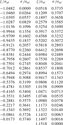
and, obviously, the hub geometry have to be prescribed. In all cases reported in this paper, the hub geometry detailed in table 1 and a value of
 $J=0.5$
are used. In addition, to properly assign the load distribution of an actuator disk with swirl the following conditions have to be satisfied:
 $$\begin{eqnarray}\displaystyle & \displaystyle \mathop{\sum }_{m=0}^{M}b_{m}=0, & \displaystyle\end{eqnarray}$$
 $$\begin{eqnarray}\displaystyle & \displaystyle b_{0}=0\quad \text{or}\quad b_{0}\neq 0\quad \text{and}\quad b_{1}=0, & \displaystyle\end{eqnarray}$$
as detailed in appendix A. Note that, for an actuator disk without wake rotation, the only condition to be met when assigning the load distribution is (3.1a
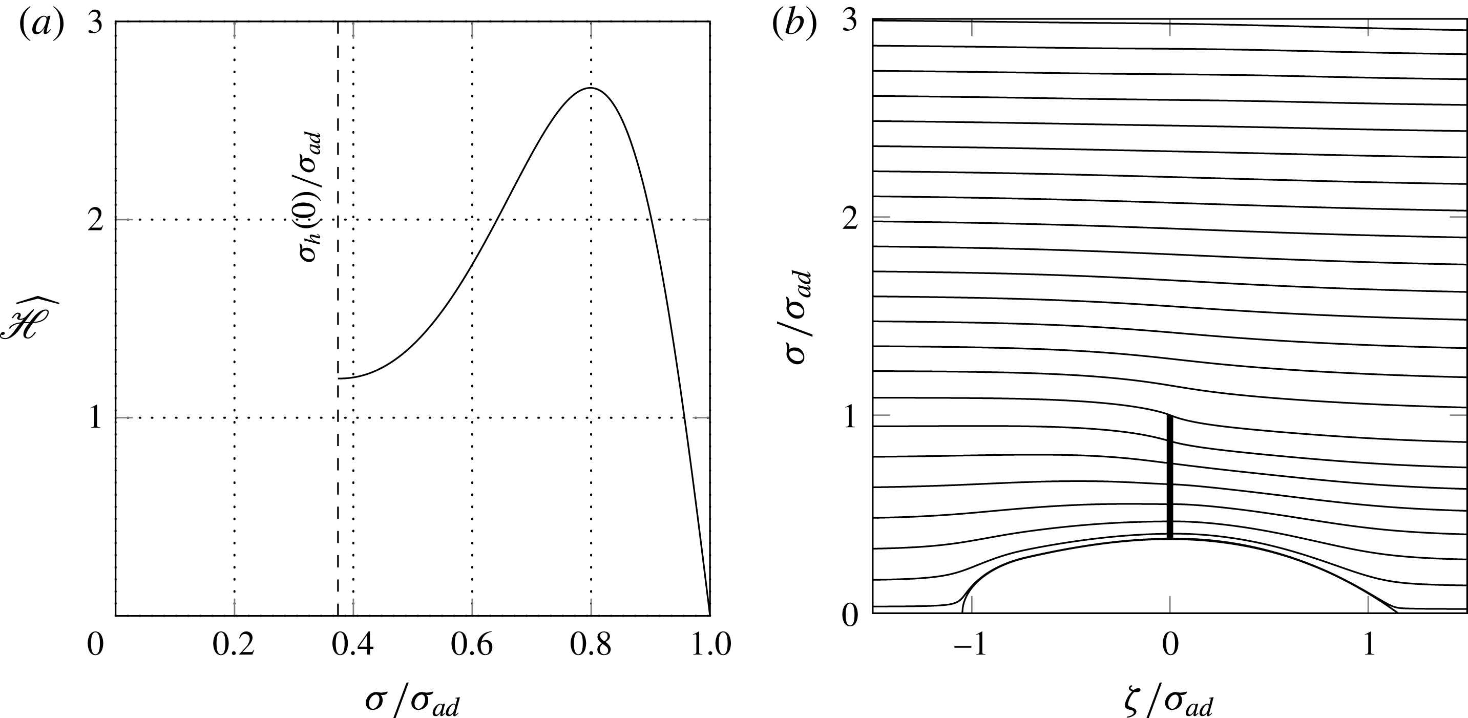
). Figure 1 shows the computed radial distribution of the load
 $\widehat{\mathscr{H}}(0,{\it\sigma}/{\it\sigma}_{ad})$
at the disk and the projection of the streamlines onto the through-flow plane obtained by prescribing
 $M=3$
,
 $b_{0}=1$
,
 $b_{1}=0$
,
 $b_{2}=10$
and
 $b_{3}=-11$
. Undoubtedly, the shape of the computed dimensionless load radial distribution
 $\widehat{\mathscr{H}}(0,{\it\sigma}/{\it\sigma}_{ad})$
has a good physical resemblance to that of a typical propeller (figure 1
a). Figure 1(b) clearly demonstrates that the no-penetration boundary condition at the hub section profile is fully satisfied. Moreover, figure 1(b) also highlights the nonlinear effect of the slipstream contraction which is completely taken into account by the present method.
Load radial distribution (a) and streamlines (b).

Hub coordinates.

Table 2 lists the predicted values of the global performance coefficients. As is customary, the following classical definitions for the thrust and power coefficients have been employed:
 $$\begin{eqnarray}C_{T,rot}=\frac{T_{rot}}{{\textstyle \frac{1}{2}}{\it\rho}U_{\infty }^{2}{\rm\pi}{\it\sigma}_{ad}^{2}},\quad C_{P}=\frac{P}{{\textstyle \frac{1}{2}}{\it\rho}U_{\infty }^{3}{\rm\pi}{\it\sigma}_{ad}^{2}},\end{eqnarray}$$
where
 $T_{rot}$
and
 $P$
are the rotor thrust and power, respectively. Moreover, the fluid also exerts a force on the hub surface. In particular, the force in the radial direction is zero for symmetry reasons, while that in the axial direction, i.e.
 $T_{hub}$
, is generally different from zero due to the presence of the propeller/turbine. In fact, without the disk vortical wake the flow must be considered as irrotational and then, from the D’Alembert’s paradox, all wall forces have to be zero. Conversely, the presence of the vortical wake region does not allow to apply the D’Alembert’s paradox, so that a thrust force on the hub may exist. Consequently, a hub thrust coefficient
 $$\begin{eqnarray}C_{T,hub}=\frac{T_{hub}}{{\textstyle \frac{1}{2}}{\it\rho}U_{\infty }^{2}{\rm\pi}{\it\sigma}_{ad}^{2}}\end{eqnarray}$$
can also be defined. With the help of the wall pressure coefficient
 $C_{p,w}=2(p-p_{\infty })/({\it\rho}U_{\infty }^{2})$
, it is easy to prove that the hub thrust coefficient can be cast in the following form (Bontempo & Manna Reference Bontempo and Manna2016b
):
 $$\begin{eqnarray}C_{T,hub}=-\frac{2\displaystyle \int _{C}p\boldsymbol{n}_{i}\boldsymbol{\cdot }\boldsymbol{i}_{{\it\zeta}}2{\rm\pi}{\it\sigma}\,\text{d}c}{{\it\rho}U_{\infty }^{2}{\rm\pi}{\it\sigma}_{ad}^{2}}=-2\int _{C}C_{p,w}\sin ({\it\beta})\frac{{\it\sigma}}{{\it\sigma}_{ad}}\,\text{d}\left(\frac{c}{{\it\sigma}_{ad}}\right),\end{eqnarray}$$
where
 $\boldsymbol{n}_{i}$
is the inward pointing normal to the hub surface and
 $\boldsymbol{i}_{{\it\zeta}}$
is the
 ${\it\zeta}$
axis unit vector. The minus sign appearing in the above equation is due to fact that
 $T_{hub}$
is customarily considered to be positive if it is concordant to
 $T_{rot}$
and vice versa. As can be appreciated in table 2, the propeller analysed in this section is characterised by a negative value of
 $C_{T,hub}$
, i.e. the fluid exerts on the hub a force opposite to the propulsive thrust. A detailed explanation for this behaviour will be provided afterwards, when the wall pressure coefficient distribution will be presented and discussed. Finally, the total thrust coefficient can be expressed as
 $C_{T}=C_{T,rot}+C_{T,hub}$
, while the propulsive efficiency is
 ${\it\eta}=C_{T}/C_{P}$
.
Semi-analytical actuator disk method: performance coefficients.

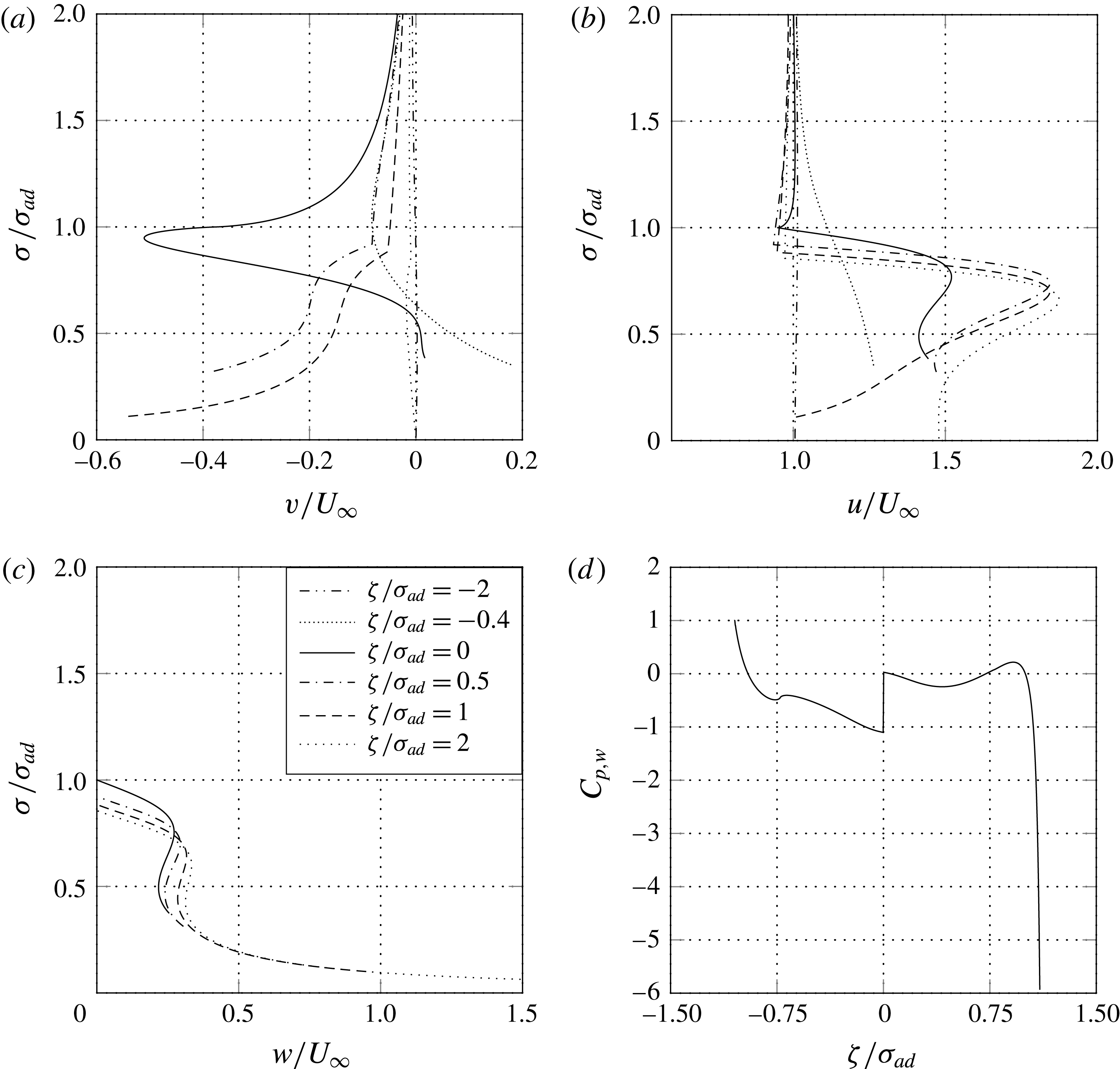
Figure 2 reports the radial distribution of the velocity components at different axial stations. More in particular, figure 2(a) shows that the radial velocity component is very small upstream and downstream the device (see the distribution of
 $v$
for
 ${\it\zeta}/{\it\sigma}_{ad}=-2$
and
 ${\it\zeta}/{\it\sigma}_{ad}=2$
). Instead, in the forepart of the hub (
 ${\it\zeta}/{\it\sigma}_{ad}=-0.4$
) the radial velocity is significant and, more precisely, it is positive near the hub and negative otherwise. This trend can be readily justified. In fact, the incoming fluid is carried outward in the spanwise direction by the forepart of the hub thus promoting a positive radial velocity. Conversely, the hub effect reduces as soon as the radius is increased and at a certain radial location the slipstream contraction effect prevails over the streamline divergence, thus giving rise to a negative radial velocity. In the back side of the hub (
 ${\it\zeta}/{\it\sigma}_{ad}=0.5,{\it\zeta}/{\it\sigma}_{ad}=1.0$
) the radial velocity is throughout negative since, in this region of the space, the hub and the slipstream contraction effects both produce a negative radial velocity.
Radial profiles of velocity components at different axial stations and wall pressure coefficient: (a) radial velocity; (b) axial velocity; (c) tangential velocity; (d) wall pressure coefficient.

Figure 2(b) shows that, for
 ${\it\zeta}/{\it\sigma}_{ad}=-2.0$
,
 $u$
is everywhere almost equal to the free stream velocity
 $U_{\infty }$
, while, for
 ${\it\zeta}/{\it\sigma}_{ad}=-0.4$
, both the hub and the actuator disk induce an increase of the axial velocity. At last, the typical propeller jet can be recognised for
 ${\it\zeta}/{\it\sigma}_{ad}\geqslant 0$
.
Figure 2(c) shows the tangential velocity radial distribution, while figure 2(d) presents the wall pressure coefficient. The
 $C_{p,w}$
jump at the disk (
 ${\it\zeta}/{\it\sigma}_{ad}=0$
) is obviously due to the non-zero value of the load at the hub
 $\mathscr{H}(0)\neq 0$
, i.e.
 $b_{0}\neq 0$
. Because of this,
 $w$
and
 $C_{p,w}$
have to approach
 $+\infty$
and
 $-\infty$
, respectively, moving towards the hub trailing edge. This can be better understood by considering that, since the hub is a stream surface,
 $\mathscr{H}$
is constant along the hub profile section from the disk
 $({\it\zeta}=0,{\it\sigma}={\it\sigma}_{h}(0))$
until the trailing edge
 $({\it\zeta}={\it\zeta}_{h,TE},{\it\sigma}=0)$
. So that, if a different from zero value of
 $\mathscr{H}$
is prescribed at the hub, namely if
 $b_{0}\neq 0$
, then
 $\mathscr{H}$
is not zero at the trailing edge. Consequently, from the angular momentum equation (2.3) the tangential velocity has to be infinite at the trailing edge, too. The same is true for the static pressure as it can be easily inferred from the definition of
 $\mathscr{H}$
. In conclusion, as is customary in all inviscid formulations, an infinite tangential velocity and wall pressure coefficient must exist at the hub trailing edge for an actuator disk with swirling wake and a rotor load different from zero at the hub. Having said that, the reason for the negative
 $C_{T,hub}$
value (see table 2) can be readily understood. In fact, as described previously,
 $C_{p,w}$
is large and negative in the trailing edge region. In this zone
 $\sin {\it\beta}$
is also negative and so, from (3.4), the trailing edge area has a predominant and negative contribution to the overall integral value of
 $C_{T,hub}$
.
The discontinuity, which appears in the radial derivative of all velocity components, is due to the discontinuity in the radial derivative of the prescribed load
 $\mathscr{H}=H-H_{\infty }$
at the slipstream edge. In fact, inside the wake,
 $\partial \mathscr{H}/\partial {\it\sigma}$
is negative near the slipstream edge (see figure 1), while it is zero outside the wake.
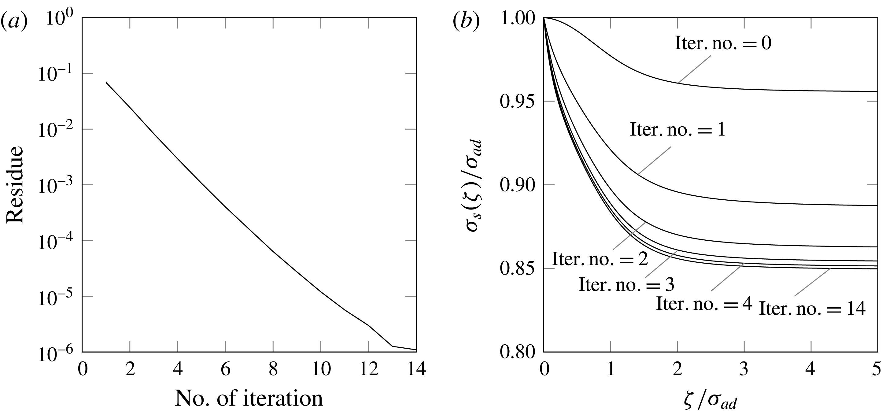
Figure 3 shows the convergence history (a) and the slipstream
 ${\it\sigma}_{s}({\it\zeta})$
at different iterations (b). The convergence rate is defined in terms of the absolute value of the difference between two successive slipstream radii evaluated at
 ${\it\zeta}=5{\it\sigma}_{ad}$
, normalised with
 ${\it\sigma}_{ad}$
. As anticipated in § 2.2, an under-relaxation technique has to be adopted in order to preserve the stability of the method. In particular, an under-relaxation factor
 ${\it\omega}_{rf}=0.5$
has been employed with success in all calculations. Figure 3 also shows that the nonlinear effects produce a significant contraction of the slipstream radius that reaches 85 % of the propeller radius at
 ${\it\zeta}/{\it\sigma}_{ad}=5$
.
Convergence analysis.

4 Error analysis and comparison with CFD
In the following section the results obtained with the semi-analytical actuator disk method are analysed and compared with those provided by a CFD-based approach. Two different cases are analysed. The first is an actuator disk without slipstream rotation and with the following values for the load distribution parameters defined in § 2.2:
 $M=3$
,
 $b_{0}=0.5$
,
 $b_{1}=1$
,
 $b_{2}=6$
and
 $b_{3}=-7.5$
. The second is an actuator disk with slipstream rotation (
 $J=0.5$
) and characterised by the following load parameters:
 $M=3$
,
 $b_{0}=0$
,
 $b_{1}=0$
,
 $b_{2}=6$
and
 $b_{3}=-6$
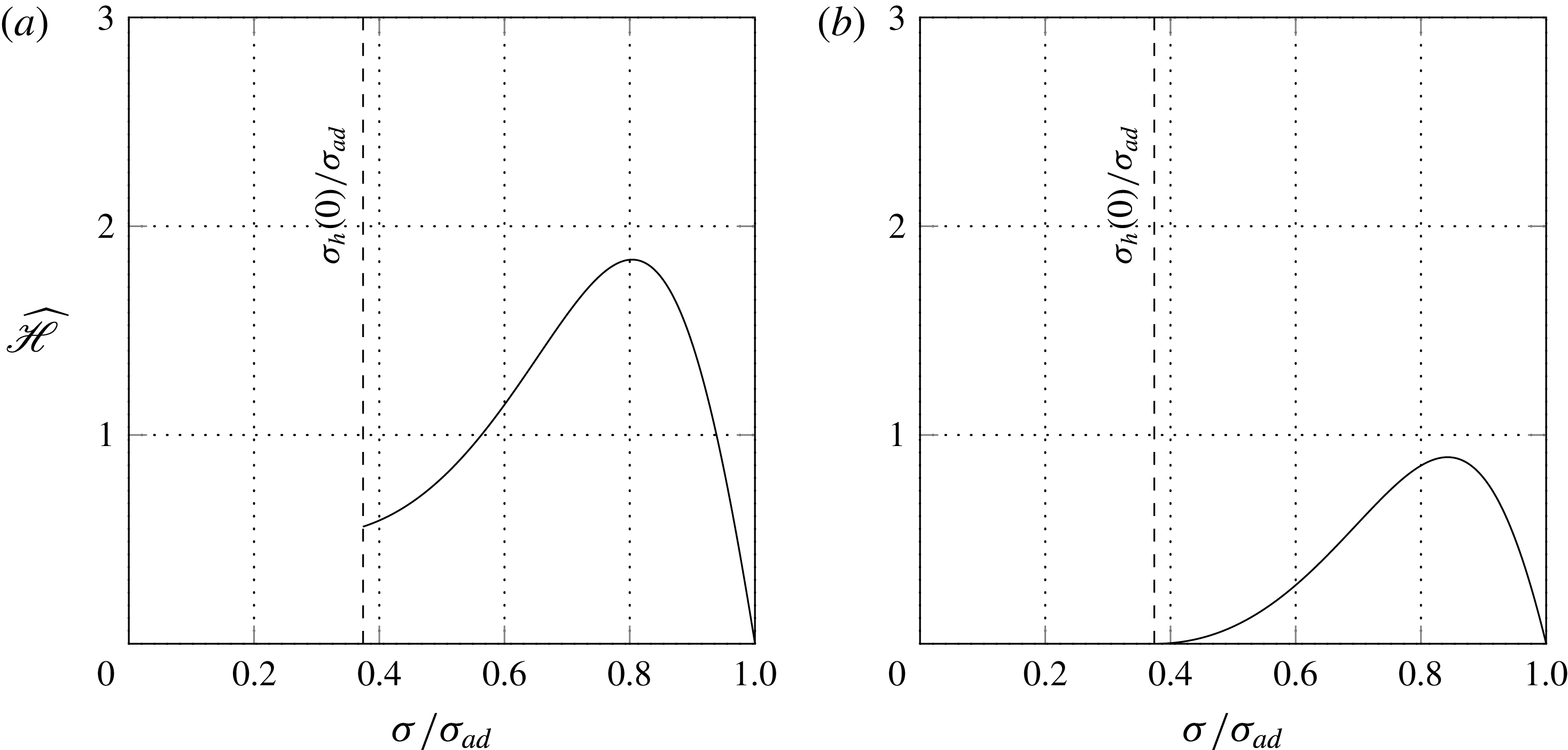
. Tables 3 and 4 list the performance coefficients related to these configurations, while the load radial distributions are shown in figure 4.
Load radial distributions: (a) without swirl (SA-5); (b) with swirl (
 $\text{SA}_{sw}$
-5).

Semi-analytical actuator disk method without slipstream rotation employed in § 4 (SA-5): performance coefficients.

Semi-analytical actuator disk method with slipstream rotation employed in § 4 (
 $\text{SA}_{sw}$
-5): performance coefficients.

In order to properly compare the results of the two methods, a detailed analysis of the numerical errors associated with the semi-analytical procedure described in § 2.2 is carried out in § 4.1. The error analysis allows to obtain a set of reference numerical data which can be compared with the results of a CFD actuator disk. The latter is a widely employed analysis tool that provides the solution of the discretised flow equations by simulating the rotor effects with a body forces distribution in the actuator disk plane. In particular, a mesh dependence analysis is first carried out in § 4.2 and then, in § 4.3, the results of the semi-analytical and CFD actuator disk methods are compared.
4.1 The nonlinear and semi-analytical actuator disk method: error analysis
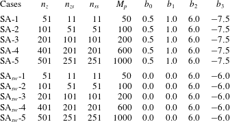
The solution procedure described in § 2.2 consists of both analytical and numerical steps. In order to gain some confidence on the accuracy of the present method, it is important to quantify the impact of the numerical errors associated with the solution procedure onto the quality of the results. To this end, the effects of the four parameters
 $n_{z}$
,
 $n_{zs}$
,
 $n_{rs}$
and
 $M_{p}$
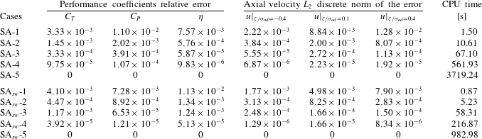
, introduced in § 2.2, are investigated and discussed. In particular, for the sake of conciseness, these parameters are made to grow all together in a five-level range (see table 5). For each flow analysis the accuracy of the performance coefficient values and of the velocity fields data is measured on the basis of the distance from the results obtained with the most accurate set (SA-5). In table 6, the relative errors of the performance coefficients and the axial velocity
 $L_{2}$
discrete norm of the errors are listed, where case SA-5 is assumed as a reference. In particular, if
 ${\it\varepsilon}({\it\sigma})$
is the absolute error between two radial distributions of the axial velocity, then, with the help of the trapezium rule, the discrete counterpart of the
 $L_{2}$
norm
 $\sqrt{\int _{0}^{{\it\sigma}_{ad}}{\it\varepsilon}^{2}\,\text{d}{\it\sigma}}$
reads
 $$\begin{eqnarray}\sqrt{\frac{{\rm\Delta}{\it\sigma}}{2}\left({\it\varepsilon}_{1}^{2}+2\mathop{\sum }_{i=2}^{I-1}{\it\varepsilon}_{i}^{2}+{\it\varepsilon}_{I}^{2}\right)}.\end{eqnarray}$$
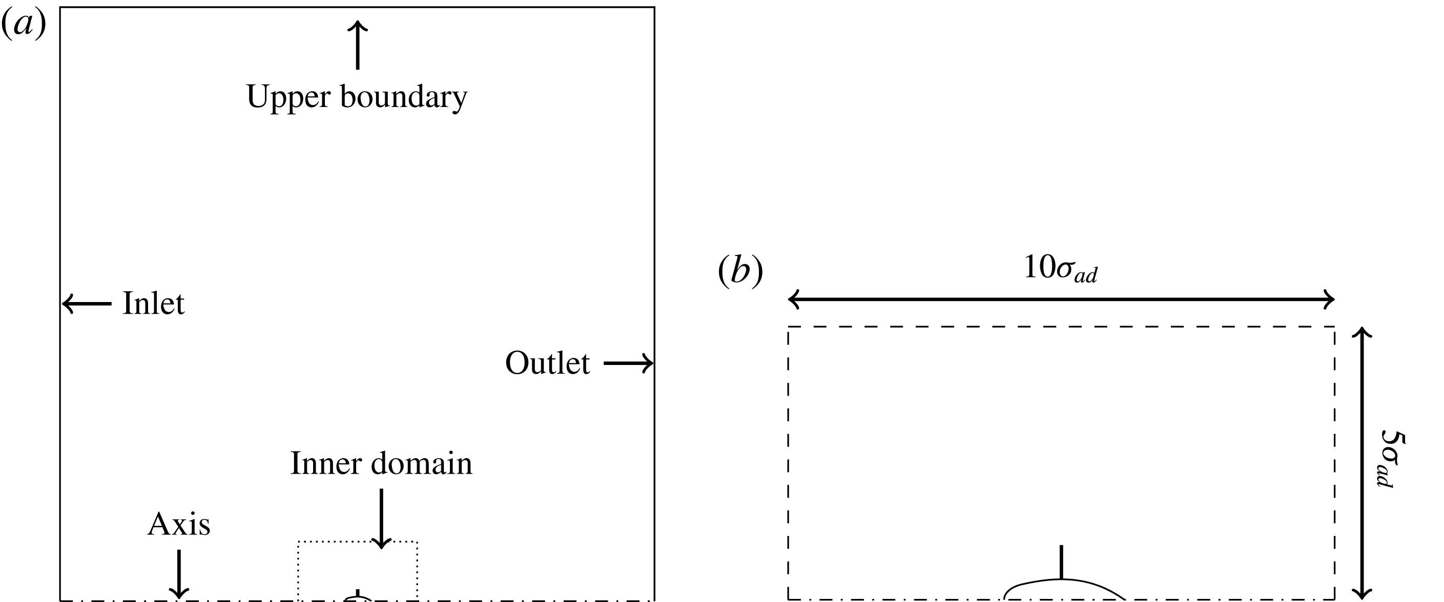
Computational domain: (a) full size; (b) inner domain.

Semi-analytical actuator disk method: numerical parameters.

Semi-analytical actuator disk method: error analysis and CPU time.

As can be easily inferred from table 6, a good accuracy level is already reached with the lowest value of the analysed numerical parameters (in both SA-1 and
 $\text{SA}_{sw}$
-1 cases the order of the relative errors for all performance coefficients is less than or equal to
 $10^{-2}$
), thus demonstrating the possibility to obtain an accurate solution in a very reduced computational time (about 1 second on an Intel Xeon CPU E5-1620 v2 3.70 GHz).
4.2 The CFD actuator disk method: mesh dependence analysis
Figure 5 shows the two-dimensional computational domain adopted in the CFD actuator disk simulations. The inlet boundary, which is located
 $25{\it\sigma}_{ad}$
ahead of the actuator disk plane, is treated as an uniform velocity boundary condition. At the outlet boundary, which is also placed
 $25{\it\sigma}_{ad}$
downstream of the rotor, a pressure-based outflow treatment is applied. At the upper boundary, which is located
 $50{\it\sigma}_{ad}$
far from the axis, and at the hub section profile an inviscid wall boundary condition is employed.
The rotor is represented through a disk-shaped region with a prescribed radial distribution of axial and tangential body forces. The axial forces return the rotor thrust when integrated over the span, while the tangential ones model the rotor torque. Obviously, these forces have to be obtained from reference cases (SA-5 and
 $\text{SA}_{sw}$
-5) of the semi-analytical method. In particular, the axial force per unit volume can be easily expressed as
 $$\begin{eqnarray}f_{{\it\zeta}}({\it\sigma})=\frac{{\rm\Delta}p({\it\sigma})}{{\rm\Delta}{\it\zeta}},\end{eqnarray}$$
where
 ${\rm\Delta}p({\it\sigma})$
is the static pressure jump across the disk and
 ${\rm\Delta}{\it\zeta}$
is the axial thickness of the disk zone in the CFD computational domain. In the swirling flow case, a radial distribution of tangential body forces must also be prescribed. From the angular momentum equation (2.3), it can be easily proven that the tangential force per unit volume is
 $$\begin{eqnarray}\displaystyle f_{{\it\theta}}({\it\sigma})=\frac{{\it\rho}u(0,{\it\sigma})w(0^{+},{\it\sigma})}{{\rm\Delta}{\it\zeta}}, & & \displaystyle\end{eqnarray}$$
where
 $u(0,{\it\sigma})$
and
 $w(0^{+},{\it\sigma})$
are the axial and tangential velocity at the disk.
Body-fitted structured multiblock meshes, generated with an elliptic solver, are used for all calculations. Different mesh densities in different parts of the computational domain have been adopted to enhance the computing efficiency. Specifically, a finer grid spacing is employed in the so-called inner domain (see figure 5 b), while the mesh density is progressively reduced moving towards the outer edges of the domain. The governing equation are solved using a pressure correction method consisting of a basic iterative procedure between the velocity and the pressure fields. Spatial discretisation is performed with a second-order scheme.
Characteristics of the mesh employed in the CFD grid dependence analysis.

Mesh dependence analysis for the CFD actuator disk method and CPU time.

The error analysis is conducted increasing the inner domain mesh density on a three-level range as detailed in table 7. Finally, table 8 reports the relative errors in the performance coefficient and the
 $L_{2}$
discrete norm of the errors in the axial velocity, assuming the fine grid level results (CFD-3 and
 $\text{CFD}_{sw}$
-3) as reference.
4.3 Comparison between the results of the semi-analytical and CFD actuator disk
As reported in Conway (Reference Conway1998), a verification procedure at downstream infinity can be carried out by means of asymptotic relations. However, such a procedure requires the knowledge of the wake radius far downstream. Instead, in the present paper, the correctness of the results is verified at all points of the computational domain and not only at downstream infinity. In particular, the results of the SA-5 (respectively
 $\text{SA}_{sw}$
-5) case have been compared with those obtained with the finest mesh CFD-3 (respectively
 $\text{CFD}_{sw}$
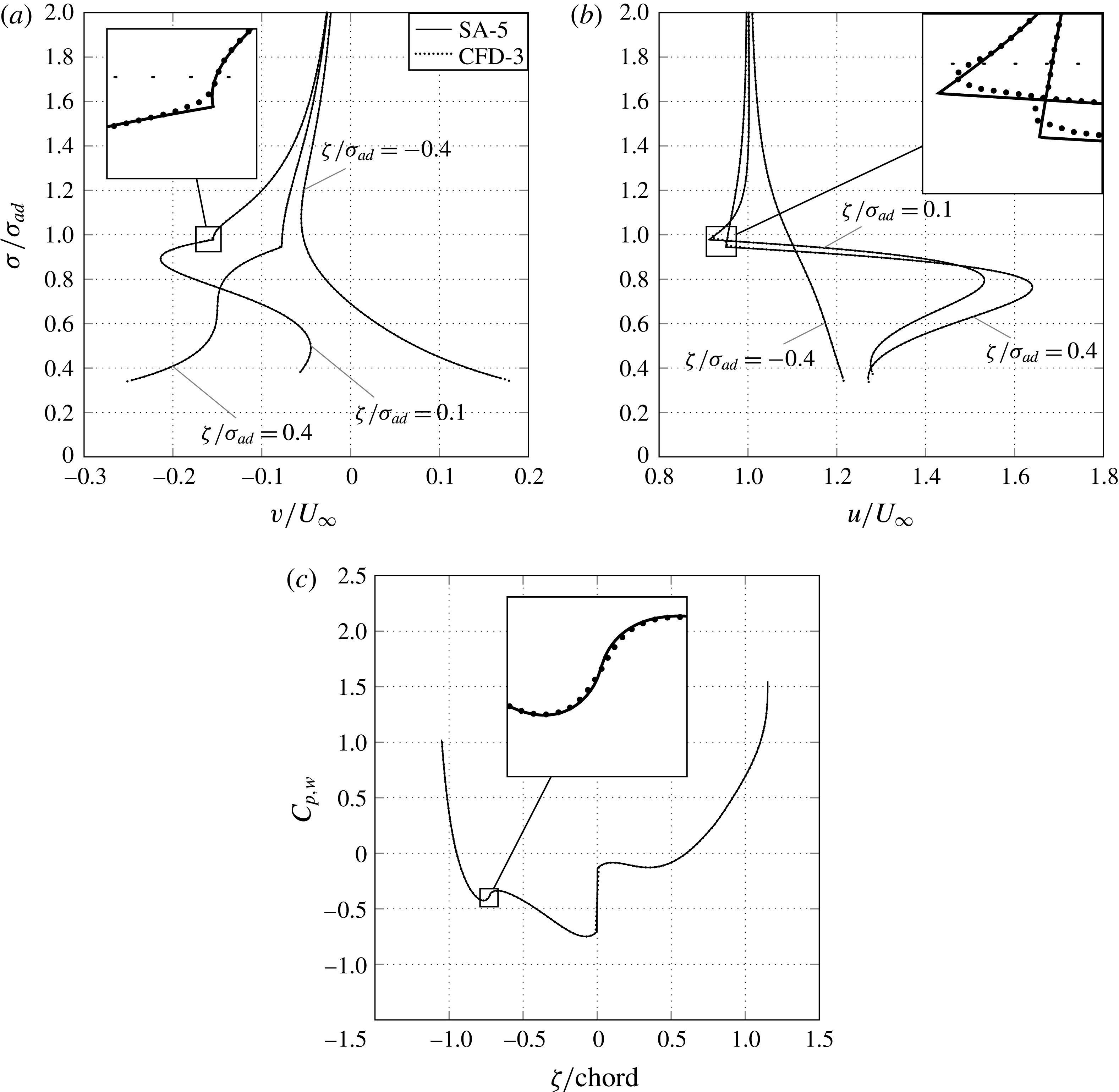
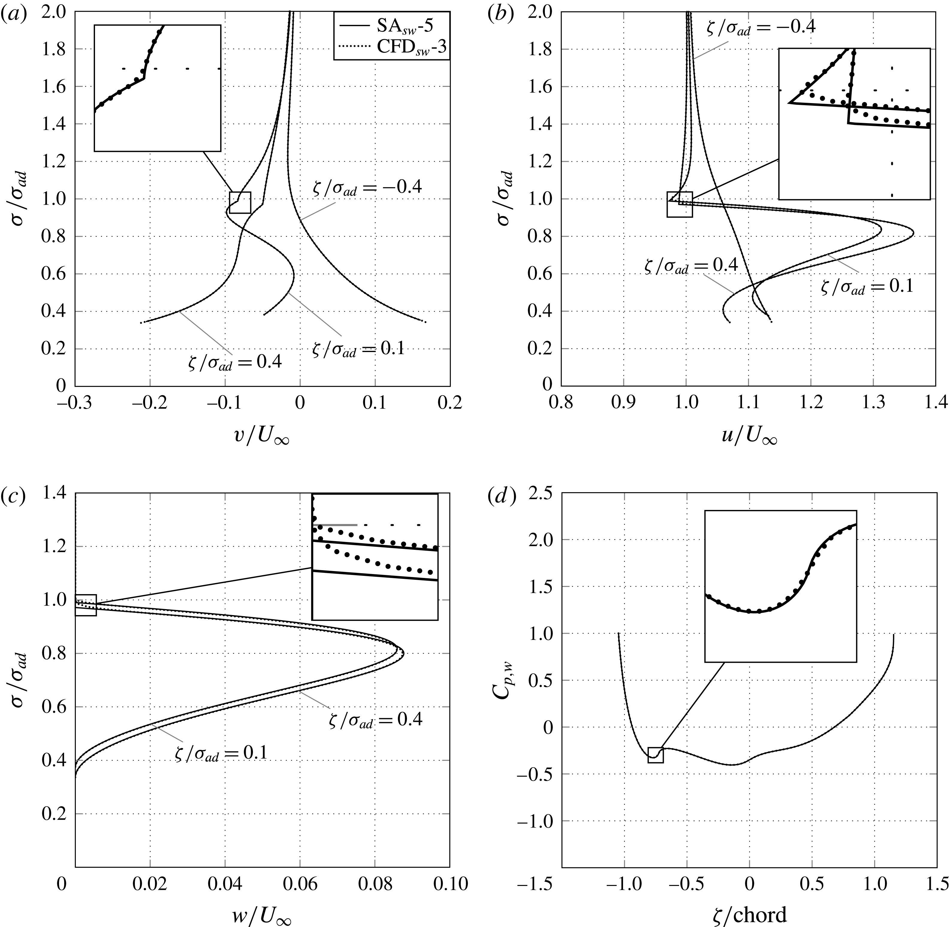
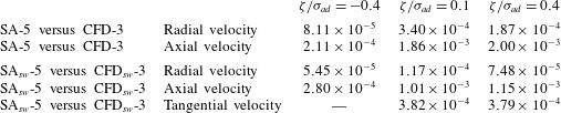
-3) through the CFD actuator disk described in the previous section. The comparisons between the velocity profiles at different axial stations and the wall pressure coefficient distributions obtained with the two methods are reported in figures 6 and 7 for the slipstream without and with swirl, respectively. In all cases the agreement is excellent as also witnessed by the errors reported in tables 9 and 10 which quantifies the differences between the results of the two models. This can be better appreciated with the help of the close-up views embedded in figures 6 and 7.
Comparison between the velocity profiles obtained with the semi-analytical (SA-5) and CFD (CFD-3) actuator disk methods: (a) radial velocity; (b) axial velocity; (c) wall pressure coefficient.

Comparison between the velocity profiles obtained with the semi-analytical (
 $\text{SA}_{sw}$
-5) and CFD (
 $\text{CFD}_{sw}$
-3) actuator disk methods: (a) radial velocity; (b) axial velocity; (c) axial velocity; (d) wall pressure coefficient.

Comparison between semi-analytical and CFD actuator disk methods:
 $L_{2}$
discrete norm of the error in the velocity components.

Comparison between semi-analytical and CFD actuator disk methods: relative error in the performance coefficients and
 $L_{2}$
discrete norm of the error in the pressure coefficient.

Also note the different behaviour of the wall pressure coefficient at the hub trailing edge in comparison to the data shown in figure 2(d). Although a rotor load different from zero is prescribed at the hub (see figure 4
a), the wall pressure coefficient is finite at the trailing edge for case SA-5 (see figure 6
c). This is obviously due to the absence of a tangential component of the velocity in the wake. In case
 $\text{SA}_{sw}$
-5, the load at the hub is zero (see figure 4
b) and then a singular behaviour of
 $w$
and
 $C_{p,w}$
is naturally avoided (see figure 7
d). As a consequence, the value of
 $C_{T,hub}$
is positive both in SA-5 and
 $\text{SA}_{sw}$
-5 cases (see tables 3 and 4).
Finally, consider the very different computational times required by the two methods (see tables 6 and 8). For example, for all performance coefficients, a relative error of the order
 $10^{-2}$
can be obtained with the numerical parameters set associated with case SA-1 and
 $\text{SA}_{sw}$
-1. The computational time is about 1 second for both cases. In contrast, a very high computational cost is required by the CFD method to obtain a result with the same accuracy (relative error of the order
 $10^{-2}$
). In fact, both cases CFD-1 and
 $\text{CFD}_{sw}$
-1 require about 500 s on the same computing platform.
5 Conclusions
In this paper the exact solution of the steady, axysimmetric, incompressible and inviscid flow around an open rotor with a hub of general shape has been derived as the superposition of ring vortices. In comparison with other simplified methods available in the open literature, the proposed approach can account for the presence of hubs of general shape, for the effects of the wake divergence/contraction and for those associated with the wake rotation. Furthermore, quite general shape of the rotor load distribution can be prescribed as input data to the method. Specifically, the load at the hub can be prescribed both equal or different from zero. In the latter case a zero value of the load radial derivative at the hub is also required to avoid a singular behaviour of the tangential vorticity on the rotor axis.
Since the exact solution is provided in an implicit formulation, an original semi-analytical and iterative procedure has been developed to make explicit the overall stream function
 ${\it\Psi}$
. The effects of the most important numerical parameters involved in the semi-analytical procedure onto the solution have also been analysed, and a set of numerical data with controlled accuracy has been obtained. Finally, the results of the semi-analytical method have been compared with those of a well-established actuator disk model based on CFD techniques. Although the two procedures are characterised by very different computational cost, an excellent agreement between the predicted flow fields has been documented.
Appendix A
This appendix deals with the features of the load distribution at the disk. First of all, as is customary in engineering applications, the load
 $\mathscr{H}$
is required to fall to zero at the disk radius
 ${\it\sigma}_{ad}$
; this implies that
 $\sum _{m=0}^{M}b_{m}=0$
(see (2.12)). Instead, the load at the hub
 $\mathscr{H}(0,{\it\sigma}_{h}(0))$
can be equal or different from zero. In particular, from (2.12), the value of the coefficient
 $b_{0}$
can be directly related to the load at the hub
 $\mathscr{H}(0,{\it\sigma}_{h}(0))$
 $$\begin{eqnarray}b_{0}=\frac{\mathscr{H}(0,{\it\sigma}_{h}(0)){\it\sigma}_{ad}^{2}}{U_{\infty }{\it\Psi}_{ad}}=\frac{\widehat{\mathscr{H}}(0,{\it\sigma}_{h}(0))}{2\widehat{{\it\Psi}}_{ad}}.\end{eqnarray}$$
Furthermore, from (2.12), it readily follows that the value of the coefficient
 $b_{1}$
is proportional to the load derivative with respect to
 ${\it\Psi}$
evaluated at the hub:
 $$\begin{eqnarray}b_{1}=\left.\frac{{\it\sigma}_{ad}^{2}}{U_{\infty }}\frac{\text{d}\mathscr{H}}{\text{d}{\it\Psi}}\right|_{{\it\Psi}=0}=\left.2\frac{\text{d}\widehat{\mathscr{H}}}{\text{d}\widehat{{\it\Psi}}}\right|_{{\it\Psi}=0}.\end{eqnarray}$$
The load
 $\mathscr{H}(0)$
and its derivative
 $\text{d}\mathscr{H}/\text{d}{\it\Psi}|_{{\it\Psi}=0}$
at the hub, i.e. the coefficients
 $b_{0}$
and
 $b_{1}$
, should enforce the boundedness of the tangential vorticity on the
 ${\it\zeta}$
axis. In fact, by prescribing both
 $\mathscr{H}(0)$
and
 $\text{d}\mathscr{H}/\text{d}{\it\Psi}|_{{\it\Psi}=0}$
different from zero at the rotor hub, it is easy to show that, as is customary in all inviscid formulations, the function
 ${\it\omega}_{{\it\theta}}/{\it\sigma}$
tends to
 $\infty$
as
 ${\it\sigma}\rightarrow 0$
, i.e. at the hub trailing edge (see the second part of (2.1)).
Instead, by assuming
 $\mathscr{H}(0)\neq 0$
and
 $\text{d}\mathscr{H}\!/\text{d}{\it\Psi}|_{{\it\Psi}=0}=0$
, (2.1) returns the indeterminate form
 $\infty \cdot 0$
as
 ${\it\sigma}\rightarrow 0$
which can be evaluated as shown in the following. The tangential component of the vorticity can be evaluated by fixing
 $b_{1}=0$
in (2.13) that, with some algebra, returns
 $$\begin{eqnarray}\lim _{{\it\sigma}\rightarrow 0}\frac{{\it\omega}_{{\it\theta}}}{{\it\sigma}}=\lim _{{\it\sigma}\rightarrow 0}\left\{\left[\frac{J^{2}{\it\Psi}}{{\rm\pi}^{2}U_{\infty }{\it\sigma}^{2}}\left(b_{0}+\mathop{\sum }_{m=2}^{M}b_{m}\left(\frac{{\it\Psi}}{{\it\Psi}_{ad}}\right)^{m-1}\right)\right]\frac{U_{\infty }}{{\it\sigma}_{ad}^{2}}\mathop{\sum }_{m=2}^{M}mb_{m}\left(\frac{{\it\Psi}}{{\it\Psi}_{ad}}\right)^{m-2}\right\}.\end{eqnarray}$$
Then, by applying the algebraic limit theorem, yields
 $$\begin{eqnarray}\lim _{{\it\sigma}\rightarrow 0}\frac{{\it\omega}_{{\it\theta}}({\it\zeta},{\it\sigma})}{{\it\sigma}}=\frac{2J^{2}}{{\rm\pi}^{2}{\it\sigma}_{ad}^{2}}b_{2}b_{0}\lim _{{\it\sigma}\rightarrow 0}\frac{{\it\Psi}}{{\it\sigma}^{2}}\end{eqnarray}$$
which results in the form
 $0/0$
. Lastly, employing the l’Hôpital’s rule and making use of the Stokes stream function definition, the tangential vorticity on the axis reads
 $$\begin{eqnarray}\lim _{{\it\sigma}\rightarrow 0}\frac{{\it\omega}_{{\it\theta}}({\it\zeta},{\it\sigma})}{{\it\sigma}}=\frac{J^{2}}{{\rm\pi}^{2}{\it\sigma}_{ad}^{2}}b_{2}b_{0}u({\it\zeta},0)\quad b_{0}\neq 0,b_{1}=0\end{eqnarray}$$
which is not a singular function.
Finally, the tangential component of the vorticity also does not exhibit a singular behaviour on the axis for
 $\mathscr{H}(0)=0$
, i.e. for
 $b_{0}=0$
. In this case the second part of (2.1) returns the indeterminate form
 $0/0$
. Fixing
 $b_{0}=0$
in (2.13) and applying the algebraic limit theorem, with some algebra, returns
 $$\begin{eqnarray}\lim _{{\it\sigma}\rightarrow 0}\frac{{\it\omega}_{{\it\theta}}({\it\zeta},{\it\sigma})}{{\it\sigma}}=\left[\frac{J^{2}}{{\rm\pi}^{2}}\frac{{\it\Psi}_{ad}}{U_{\infty }}\left(\lim _{{\it\sigma}\rightarrow 0}\frac{\displaystyle \mathop{\sum }_{m=1}^{M}b_{m}\left({\displaystyle \frac{{\it\Psi}}{{\it\Psi}_{ad}}}\right)^{m}}{{\it\sigma}^{2}}\right)-1\right]\frac{U_{\infty }}{{\it\sigma}_{ad}^{2}}b_{1}.\end{eqnarray}$$
At the end, using the l’Hôpital’s rule, the tangential vorticity on the axis becomes
 $$\begin{eqnarray}\lim _{{\it\sigma}\rightarrow 0}\frac{{\it\omega}_{{\it\theta}}({\it\zeta},{\it\sigma})}{{\it\sigma}}=\frac{U_{\infty }b_{1}}{{\it\sigma}_{ad}^{2}}\left(\frac{J^{2}}{2{\rm\pi}^{2}}b_{1}\frac{u({\it\zeta},0)}{U_{\infty }}\right),\end{eqnarray}$$
a finite value, which has been obtained enforcing
 $b_{0}=0$
.