1 Introduction
In 1935, Geoffrey Taylor outlined his statistical theory for turbulence, which included the definition of what became known as the Taylor length scale,
 $\unicode[STIX]{x1D706}$
. He stated that this length corresponds to the diameter of the smallest eddies responsible for the dissipation of energy (Taylor Reference Taylor1935). Subsequent work established that the characteristic length scale for the smallest eddies is the Kolmogorov scale,
 $\unicode[STIX]{x1D702}=(\unicode[STIX]{x1D708}^{3}/\unicode[STIX]{x1D716})^{1/4}$
, where
 $\unicode[STIX]{x1D708}$
is the kinematic viscosity and
 $\unicode[STIX]{x1D716}$
is the dissipation rate (Kolmogorov Reference Kolmogorov1941). However, there has been increasing interest in the role of the Taylor scale for turbulence dissipation in recent years in terms of spectral-based studies of energy transfer (George Reference George1992), the discovery that the Einstein–Markov coherence length for turbulence is typically
 ${\sim}0.8\unicode[STIX]{x1D706}$
(Lück et al.
Reference Lück, Renner, Peinke and Friedrich2006) and the result that the maximum dissipation length is similar to the Taylor scale and exhibits a square-root scaling with Reynolds number (Yakhot Reference Yakhot2003). In addition, there is work showing that the dissipation rate coefficient can also be related to the stagnation point structure in the flow, which in turn implies a Taylor length scaling because the mean separation of stagnation points is proportional to
 $\unicode[STIX]{x1D706}$
(Goto & Vassilicos Reference Goto and Vassilicos2009). Hence, the fluctuating velocity is much rougher at scales larger than
 $\unicode[STIX]{x1D706}$
than at smaller scales, providing the rationale for intermittency-based studies of turbulence (Batchelor & Townsend Reference Batchelor and Townsend1949; Kolmogorov Reference Kolmogorov1962; Frisch, Sulem & Nelkin Reference Frisch, Sulem and Nelkin1978; Meneveau & Sreenivasan Reference Meneveau and Sreenivasan1987; Lashermes et al.
Reference Lashermes, Roux, Abry and Jaffard2008). The link that Goto & Vassilicos (Reference Goto and Vassilicos2009) established between dissipation coefficient and stagnation structure is a statement about flow topology because the large eddies in the flow determine this structure. Research undertaken by Elsinga & Marusic (Reference Elsinga and Marusic2010) looked into the small-scale properties of turbulent boundary layers, channel flows and homogeneous, isotropic turbulence (HIT), using simulations and particle imaging velocimetry data. Their results supported a model for turbulence where vortices are found at the edge of uniform flow regions, and for all flows studied, the distance between vortex cores was between
 $1.4\unicode[STIX]{x1D706}$
and
 $1.8\unicode[STIX]{x1D706}$
, consistent with the imprint of the large eddies on the stagnation point structure.
It is not immediately clear from the basic equations why such structures play a role in dissipation because local dissipation is defined as
 $$\begin{eqnarray}\unicode[STIX]{x1D716}=\unicode[STIX]{x1D708}\,\text{tr}(\unicode[STIX]{x1D64E}_{A}^{2}),\end{eqnarray}$$
where the strain rate is
 $$\begin{eqnarray}\unicode[STIX]{x1D64E}_{A}={\textstyle \frac{1}{2}}(\unicode[STIX]{x1D63C}+\unicode[STIX]{x1D63C}^{\ast }),\end{eqnarray}$$
with the velocity gradient tensor (VGT),
 $\unicode[STIX]{x1D63C}$
, is given by
 $\unicode[STIX]{x1D608}_{ij}=\unicode[STIX]{x2202}u_{i}/\unicode[STIX]{x2202}x_{j}$
, where
 $u$
is an orthogonal velocity component,
 $x$
is an orthogonal spatial direction and the asterisk is the transpose. To complete this picture, the additive decomposition of the VGT into Hermitian (strain rate) and skew-Hermitian (rotation rate) components is
 $$\begin{eqnarray}\unicode[STIX]{x1D63C}=\unicode[STIX]{x1D64E}_{A}+\unicode[STIX]{x03A9}_{A},\end{eqnarray}$$
where
 $$\begin{eqnarray}\unicode[STIX]{x03A9}_{A}={\textstyle \frac{1}{2}}(\unicode[STIX]{x1D63C}-\unicode[STIX]{x1D63C}^{\ast }).\end{eqnarray}$$
While (1.1) shows that rotation rate, vorticity or enstrophy plays no direct role in local dissipation, the equation for the evolution of the total strain contains terms corresponding to both strain production,
 $-\text{det}(\unicode[STIX]{x1D64E}_{A})$
, and enstrophy production,
 $\text{tr}(\unicode[STIX]{x03A9}_{A}^{2}\unicode[STIX]{x1D64E}_{A})$
, (Tsinober Reference Tsinober, Hunt and Vassilicos2001)
 $$\begin{eqnarray}\frac{1}{2}\frac{\text{D}\,\text{tr}(\unicode[STIX]{x1D64E}_{A}^{2})}{\text{D}t}=-3\,\text{det}(\unicode[STIX]{x1D64E}_{A})-\frac{1}{4}\text{tr}(\unicode[STIX]{x03A9}_{A}^{2}\unicode[STIX]{x1D64E}_{A})-\unicode[STIX]{x1D64E}_{A}\frac{\unicode[STIX]{x2202}^{2}p}{\unicode[STIX]{x2202}x_{i}\unicode[STIX]{x2202}x_{j}}+\unicode[STIX]{x1D708}\unicode[STIX]{x1D64E}_{A}\unicode[STIX]{x1D6FB}^{2}\unicode[STIX]{x1D64E}_{A},\end{eqnarray}$$
and there is a long history to considering the role of enstrophy production in dissipation physics (Taylor Reference Taylor1938a ). In particular, the relative alignment between the vortical and straining components of the flow are a crucial for determining the magnitude of this term (Hamlington, Schumacher & Dahm Reference Hamlington, Schumacher and Dahm2008). A key result from the early numerical investigations into the properties of HIT was the preferential alignment between the vorticity vector and the strain eigenvector corresponding to the intermediate strain eigenvalue (Kerr Reference Kerr1985; Ashurst et al. Reference Ashurst, Kerstein, Kerr and Gibson1987). Ohkitani (Reference Ohkitani2002) has shown the importance of viscosity for preserving this alignment between the vorticity vector and the intermediate eigenvector, highlighting the limitations of models based on the Euler equations for capturing the full dynamics of turbulence. While the evolution of total strain is (indirectly) dependent on enstrophy production and, thus, the behaviour of vortices in the flow, the evolution of the enstrophy itself is directly proportional to the enstrophy production
 $$\begin{eqnarray}\frac{1}{2}\frac{\text{D}\,\text{tr}(\unicode[STIX]{x03A9}_{A}^{2})}{\text{D}t}=\text{tr}(\unicode[STIX]{x03A9}_{A}^{2}\unicode[STIX]{x1D64E}_{A})+\unicode[STIX]{x1D708}\unicode[STIX]{x03A9}_{A}\unicode[STIX]{x1D6FB}^{2}\unicode[STIX]{x03A9}_{A},\end{eqnarray}$$
and the mean enstrophy production,
 $\langle \text{tr}(\unicode[STIX]{x03A9}_{A}^{2}\unicode[STIX]{x1D64E}_{A})\rangle$
is positive (Taylor Reference Taylor1938a
).
This paper is concerned with the role of vortical motions in dissipation physics, but is focussed on the partitioning of the total strain and enstrophy at a point in the flow field between local and non-local processes. Non-locality is, with nonlinearity and non-integrability, one of the ‘three Ns’ of turbulence (Tsinober Reference Tsinober2009) that make the analysis of the Navier–Stokes equations so difficult. The novel aspect of our approach is to introduce a mathematical bound on the behaviour of the VGT. We then examine the manner in which the bound is attained, and the typical statistics for the flow when the bound is attained compared with other times and locations. We show that the Taylor scale plays a role in determining the maximum size of the regions that attain the bound and, how the genuinely local contribution to strain virtually disappears in such regions, while the values for total strain and the production terms,
 $\text{tr}(\unicode[STIX]{x03A9}_{A}^{2}\unicode[STIX]{x1D64E}_{A})$
and
 $-\text{det}(\unicode[STIX]{x1D64E}_{A})$
, remain essentially constant. In other words, there is an intermittency to dissipation, not in terms of the standard conceptualisation of this phenomenon (Kolmogorov Reference Kolmogorov1962; Frisch et al.
Reference Frisch, Sulem and Nelkin1978), but in terms of the partitioning of the total strain between local and non-local contributions and the decline of the former.
2 The Lee bound for the velocity gradient tensor
There are typically two approaches to the analysis of turbulent flows in terms of the VGT. The first focusses on the decomposition into strain rate and rotation rate tensors as discussed above, where it is also common to express the rotation tensor as a vorticity vector,
 $\unicode[STIX]{x1D74E}$
, where each term is
 $$\begin{eqnarray}\unicode[STIX]{x1D714}_{i}^{(A)}=-\unicode[STIX]{x1D716}_{ijk}\unicode[STIX]{x1D6FA}_{jk}^{(A)},\end{eqnarray}$$
and
 $\unicode[STIX]{x1D716}_{ijk}$
is the Levi-Cevita symbol. The second approach considers the invariants of the characteristic equation of
 $\unicode[STIX]{x1D63C}$
 $$\begin{eqnarray}e_{i}^{3}+P_{A}e_{i}^{2}+Q_{A}e_{i}+R_{A}=0,\end{eqnarray}$$
which intrinsically requires a consideration of the eigenvalues,
 $e_{i}$
. For incompressible turbulence,
 $P_{A}=-\sum e_{i}=0$
, leading to a compact expression for the discriminant function separating regions where the eigenvalues are real (
 $\unicode[STIX]{x1D6E5}<0$
) and where they form a conjugate pair (
 $\unicode[STIX]{x1D6E5}>0$
) (Chong, Perry & Cantwell Reference Chong, Perry and Cantwell1990; Rabey, Wynn & Buxton Reference Rabey, Wynn and Buxton2015):
 $$\begin{eqnarray}\unicode[STIX]{x1D6E5}=Q_{A}^{3}+{\textstyle \frac{27}{4}}R_{A}^{2}.\end{eqnarray}$$
It is then possible to write equations for the Lagrangian evolution of the flow in terms of the remaining two invariants, and their constituent terms (Girimaji & Pope Reference Girimaji and Pope1990; Martin, Dopazo & Valiño Reference Martin, Dopazo and Valiño1998; Biferale et al. Reference Biferale, Chevillard, Meneveau and Toschi2007; Li & Meneveau Reference Li and Meneveau2007; Chevillard et al. Reference Chevillard, Meneveau, Biferale and Toschi2008; Wilczek & Meneveau Reference Wilczek and Meneveau2014; Johnson & Meneveau Reference Johnson and Meneveau2016). The most celebrated approach due to the need to only consider the invariants is the restricted Euler model (Cantwell Reference Cantwell1992)
 $$\begin{eqnarray}\displaystyle & \displaystyle \frac{\text{d}Q_{A}}{\text{d}t}=-3R_{A} & \displaystyle\end{eqnarray}$$
 $$\begin{eqnarray}\displaystyle & \displaystyle \frac{\text{d}R_{A}}{\text{d}t}=\frac{2}{3}Q_{A}^{2}, & \displaystyle\end{eqnarray}$$
where it is assumed that viscous effects may be ignored and that the pressure Hessian is isotropic. This model replicates a number of the features of turbulence (Meneveau Reference Meneveau2011), but cannot capture the observed clockwise circulation of Lagrangian trajectories around a space formed from
 $Q_{A}$
and
 $R_{A}$
, which is demonstrated later in this paper. This is because trajectories maintain a constant value for
 $\unicode[STIX]{x1D6E5}$
in the restricted Euler model. In addition, the model is unable to capture the role of viscous effects (Ohkitani Reference Ohkitani2002) or the deviatoric part of the pressure Hessian on the preservation of the alignment between the vorticity vector and the intermediate strain eigenvector.
It has recently been suggested that there are advantages in introducing an additive decomposition of the velocity gradient tensor,
 $\unicode[STIX]{x1D63C}=\unicode[STIX]{x1D63D}+\unicode[STIX]{x1D63E}$
that isolates the eigenvalue-related normal contributions in
 $\unicode[STIX]{x1D63D}$
, with
 $\unicode[STIX]{x1D63E}$
containing the non-normal contributions (Keylock Reference Keylock2018). This approach is based on a complex Schur decomposition of
 $\unicode[STIX]{x1D63C}$
(Schur Reference Schur1909), given by
 $$\begin{eqnarray}\unicode[STIX]{x1D63C}=\unicode[STIX]{x1D650}\unicode[STIX]{x1D64F}\unicode[STIX]{x1D650}^{\ast },\end{eqnarray}$$
where
 $\unicode[STIX]{x1D650}$
is unitary and the upper triangular tensor
 $\unicode[STIX]{x1D64F}=\unicode[STIX]{x1D640}+\unicode[STIX]{x1D649}$
consists of a diagonal matrix of eigenvalues,
 $\unicode[STIX]{x1D640}$
, where
 $E_{i,i}=e_{i}$
, and the non-normal contribution,
 $\unicode[STIX]{x1D649}$
. Decomposing
 $\unicode[STIX]{x1D64F}$
in this way leads to
 $$\begin{eqnarray}\displaystyle \left.\begin{array}{@{}c@{}}\unicode[STIX]{x1D63D}=\unicode[STIX]{x1D650}\unicode[STIX]{x1D640}\unicode[STIX]{x1D650}^{\ast }\\ \unicode[STIX]{x1D63E}=\unicode[STIX]{x1D650}\unicode[STIX]{x1D649}\unicode[STIX]{x1D650}^{\ast }.\end{array}\right\} & & \displaystyle\end{eqnarray}$$
This permits, for example, a simple rewriting of the restricted Euler model as
 $$\begin{eqnarray}\displaystyle & \displaystyle \frac{\text{d}Q_{B}}{\text{d}t}=-3R_{B} & \displaystyle\end{eqnarray}$$
 $$\begin{eqnarray}\displaystyle & \displaystyle \frac{\text{d}R_{B}}{\text{d}t}=\frac{2}{3}Q_{B}^{2}. & \displaystyle\end{eqnarray}$$
That the non-normal contributions from
 $\unicode[STIX]{x1D63E}$
are excluded from the restricted Euler model highlights that the effects captured in the non-normal term are those due to the deviatoric part of the pressure Hessian, i.e. the non-local aspects of the turbulence structure (Ohkitani & Kishiba Reference Ohkitani and Kishiba1995; Hamlington et al.
Reference Hamlington, Schumacher and Dahm2008). The equation for
 $Q_{A}$
may be written as
 $$\begin{eqnarray}Q_{A}={\textstyle \frac{1}{2}}(\Vert \unicode[STIX]{x03A9}_{A}\Vert ^{2}-\Vert \unicode[STIX]{x1D64E}_{A}\Vert ^{2}),\end{eqnarray}$$
where, e.g.
 $\Vert \unicode[STIX]{x1D64E}_{A}\Vert \equiv \sqrt{\text{tr}(\unicode[STIX]{x1D64E}_{A}\unicode[STIX]{x1D64E}_{A}^{\ast })}$
is the Frobenius norm. The equivalent expression for
 $R_{A}$
is
 $$\begin{eqnarray}R_{A}=-\text{det}(\unicode[STIX]{x1D64E}_{A})-\text{tr}(\unicode[STIX]{x03A9}_{A}^{2}\unicode[STIX]{x1D64E}_{A}),\end{eqnarray}$$
and the full set of five ordinary differential equations for the evolution of the velocity gradient tensor (Martin et al.
Reference Martin, Dopazo and Valiño1998) consists of the semi-autonomous pair of equations given in (2.4) and (2.5) as well as evolution equation for the total strain,
 $\Vert \boldsymbol{S}_{A}\Vert ^{2}$
, and strain production,
 $-\text{det}(\unicode[STIX]{x1D64E}_{A})$
, and the square of the vortex stretching vector,
 $V=\unicode[STIX]{x1D74E}_{A}\unicode[STIX]{x1D64E}_{A}$
(Tsinober, Shtilman & Vaisburd Reference Tsinober, Shtilman and Vaisburd1997). This system of five equations is derived by using (2.10) and (2.11) to eliminate equations for the enstrophy,
 $\Vert \unicode[STIX]{x03A9}_{A}\Vert ^{2}$
and enstrophy production
 $\text{tr}(\unicode[STIX]{x03A9}_{A}^{2}\unicode[STIX]{x1D64E}_{A})$
. It is through these latter three evolution equations that non-normality is captured, not via (2.10) and (2.11). This is explained in greater detail in the text surrounding (3.1)–(3.4), below.
2.1 Non-normality and the Lee bound
Taking the Frobenius norm of
 $\unicode[STIX]{x1D649}$
, i.e.
 $n=\Vert \unicode[STIX]{x1D649}\Vert$
gives one form for tensor non-normality. An alternative is given by
 $$\begin{eqnarray}h=\Vert \unicode[STIX]{x1D63C}\unicode[STIX]{x1D63C}^{\ast }-\unicode[STIX]{x1D63C}^{\ast }\unicode[STIX]{x1D63C}\Vert ,\end{eqnarray}$$
and there has been a significant amount of work formulating bounds for
 $n$
given
 $h$
or vice versa (Henrici Reference Henrici1962; Eberlein Reference Eberlein1965; Kress, De Vies & Wegmann Reference Kress, De Vies and Wegmann1974). A tight bound was proposed by Lee (Reference Lee1995), which considers complex shifts of
 $\unicode[STIX]{x1D63C}$
and also uses the Hermitian/skew-Hermitian decomposition of the tensor. The latter is important because non-normality is partitioned equally between strain and rotation components in this frame (Keylock Reference Keylock2018; Dong, Gao & Liu Reference Dong, Gao and Liu2019), leading to
 $$\begin{eqnarray}\displaystyle \left.\begin{array}{@{}c@{}}\displaystyle \Vert \unicode[STIX]{x1D64E}_{A}\Vert ^{2}=\Vert \text{Re}\{\unicode[STIX]{x1D640}\}\Vert ^{2}+{\textstyle \frac{1}{2}}\Vert \unicode[STIX]{x1D649}\Vert ^{2}\\ \displaystyle \Vert \unicode[STIX]{x03A9}_{A}\Vert ^{2}=\Vert \text{Im}\{\unicode[STIX]{x1D640}\}\Vert ^{2}+{\textstyle \frac{1}{2}}\Vert \unicode[STIX]{x1D649}\Vert ^{2},\end{array}\right\} & & \displaystyle\end{eqnarray}$$
where
 $\text{Re}$
and
 $\text{Im}$
are the real and imaginary parts.
Introducing a complex scalar,
 $\unicode[STIX]{x1D6FC}$
, such that the perturbed VGT is
 $\unicode[STIX]{x1D63C}-\unicode[STIX]{x1D6FC}\unicode[STIX]{x1D644}$
, where
 $\unicode[STIX]{x1D644}$
is the identity matrix, the perturbed strain and rotation tensors are given, respectively, by
 $\unicode[STIX]{x1D64E}_{A}-\text{Re}(\unicode[STIX]{x1D6FC})\unicode[STIX]{x1D644}$
and
 $\unicode[STIX]{x03A9}_{A}-\text{Im}(\unicode[STIX]{x1D6FC})\unicode[STIX]{x1D644}$
. The upper Lee bound for
 $n$
,
 $b^{L}(n)$
, is
 $$\begin{eqnarray}b^{L}(n)=b^{L}(\unicode[STIX]{x1D63C}-\unicode[STIX]{x1D6FC}\unicode[STIX]{x1D644})=\text{min}\left\{\begin{array}{@{}c@{}}\sqrt{2}(\Vert \unicode[STIX]{x1D64E}_{A}-\text{Re}\{\unicode[STIX]{x1D6FC}\}\unicode[STIX]{x1D644}\Vert ^{2}-\Vert \text{Re}\{\unicode[STIX]{x1D640}\}-\text{Re}\{\unicode[STIX]{x1D6FC}\}\unicode[STIX]{x1D644}\Vert ^{2})^{1/2}\\ \sqrt{2}(\Vert \unicode[STIX]{x03A9}_{A}-i\text{Im}\{\unicode[STIX]{x1D6FC}\}\unicode[STIX]{x1D644}\Vert ^{2}-\Vert \text{Im}\{\unicode[STIX]{x1D640}\}-\text{Im}\{\unicode[STIX]{x1D6FC}\}\unicode[STIX]{x1D644}\Vert ^{2})^{1/2}.\end{array}\right.\end{eqnarray}$$
Taking each of these expressions and minimising the term containing the eigenvalues establishes that
 $$\begin{eqnarray}\unicode[STIX]{x1D6FC}=\frac{1}{3}\sum \text{Re}\{e_{i}\}+\frac{1}{3}i\sum \text{Im}\{e_{i}\}=\frac{1}{3}\text{tr}(\unicode[STIX]{x1D63C}).\end{eqnarray}$$
For incompressible turbulence, where
 $\text{tr}(\unicode[STIX]{x1D63C})=0$
, the Lee bound may be simplified to the following, tight expression:
 $$\begin{eqnarray}b^{L}(n)\leqslant \sqrt{2}\min (\Vert \unicode[STIX]{x1D64E}_{A}\Vert ,\Vert \unicode[STIX]{x03A9}_{A}\Vert ).\end{eqnarray}$$
In terms of the invariants in (2.2), and given (2.10), it follows that
 $\Vert \unicode[STIX]{x1D64E}_{A}\Vert$
will control the bound in rotational regions with positive
 $Q_{A}$
, and
 $\Vert \unicode[STIX]{x03A9}_{A}\Vert$
dictates the bound for negative
 $Q_{A}$
. Beneath the discriminant function, where
 $\unicode[STIX]{x1D6E5}<0$
, it can be shown that
 $\Vert \unicode[STIX]{x03A9}_{B}\Vert =0$
(Keylock Reference Keylock2018). Given the equipartition of non-normality between strain and rotation in (2.13) it then follows from (2.16) that for
 $\unicode[STIX]{x1D6E5}<0$
,
 $b^{L}=\sqrt{2}\Vert \unicode[STIX]{x03A9}_{C}\Vert =\sqrt{2}\Vert \unicode[STIX]{x1D64E}_{C}\Vert$
. Hence, the Lee bound must be fulfilled in this region. However, where
 $\unicode[STIX]{x1D6E5}>0$
no such constraint exists and the attainment of the bound in these vortical regions is non-trivial. This forms the focus of this paper.
2.2 Vortical flow regions and attainment of the Lee bound
In this paper, for consistency with the above statement, we adopt a common, practical definition of a vortical region in the flow as one where a conjugate pair of eigenvalues exists, i.e.
 $\unicode[STIX]{x1D6E5}>0$
(Chong et al.
Reference Chong, Perry and Cantwell1990). This means that in the Lagrangian frame, there is a closed streamline. Such a definition also underpins other measures of coherent structures that are based on the imaginary part of the eigenvalues (Zhou et al.
Reference Zhou, Adrian, Balachandar and Kendall1999; Chakraborty, Balachandar & Adrian Reference Chakraborty, Balachandar and Adrian2005). Thus, given
 $\unicode[STIX]{x1D6E5}>0$
, we can define the degree to which the Lee bound is attained as
 $$\begin{eqnarray}\unicode[STIX]{x1D6F7}=\frac{\Vert \unicode[STIX]{x1D649}\Vert }{\sqrt{2}\min (\Vert \unicode[STIX]{x1D64E}_{A}\Vert ,\Vert \unicode[STIX]{x03A9}_{A}\Vert )},\end{eqnarray}$$
where the implication of (2.10) for (2.17) is that where
 $Q_{A}>0$
the bound is imposed by
 $\Vert \unicode[STIX]{x1D64E}_{A}\Vert$
and where
 $Q_{A}<0$
it is based on
 $\Vert \unicode[STIX]{x03A9}_{A}\Vert$
, with the bound obtained in a trivial fashion for
 $\unicode[STIX]{x1D6E5}<0$
. From this, we consider the practical attainment of the Lee bound to be indicated by the binary variable,
 $\ell$
, where
 $$\begin{eqnarray}\displaystyle \left.\begin{array}{@{}c@{}}\displaystyle \ell =1\quad \text{if}~\unicode[STIX]{x1D6F7}>0.9999\\ \displaystyle \ell =0\quad \text{if}~\unicode[STIX]{x1D6F7}\leqslant 0.9999.\end{array}\right\} & & \displaystyle\end{eqnarray}$$
3 Numerical simulation and Eulerian results
3.1 Direct numerical simulation
This study makes use of the Johns Hopkins Turbulence Database direct numerical simulation of steady HIT at a Taylor Reynolds number of 433 (Li et al.
Reference Li, Perlman, Wan, Yang, Burns, Meneveau, Chen, Szalay and Eyink2008; Wan et al.
Reference Wan, Chen, Eyink, Meneveau, Perlman, Burns, Li, Szalay and Hamilton2016), which has been employed in a number of other turbulence studies (Lüthi, Holzner & Tsinober Reference Lüthi, Holzner and Tsinober2009; Wan et al.
Reference Wan, Xiao, Meneveau, Eyink and Chen2010; Keylock Reference Keylock2017; Ballouz & Ouellette Reference Ballouz and Ouellette2018). The simulation was performed on a
 $1024^{3}$
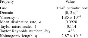
grid using a pseudo-spectral method. The energy was injected to maintain the total energy in the Fourier modes, while also retaining a wavenumber magnitude less than or equal to 2 in each mode. Some properties of the simulation are summarised in table 1.
Summary properties of the HIT simulation in the Johns Hopkins database (Li et al. Reference Li, Perlman, Wan, Yang, Burns, Meneveau, Chen, Szalay and Eyink2008). All quantities are dimensionless.

3.2 Attainment of the Lee bound in
 $Q_{A}-R_{A}$
space

A sketch of the
 $Q_{A}-R_{A}$
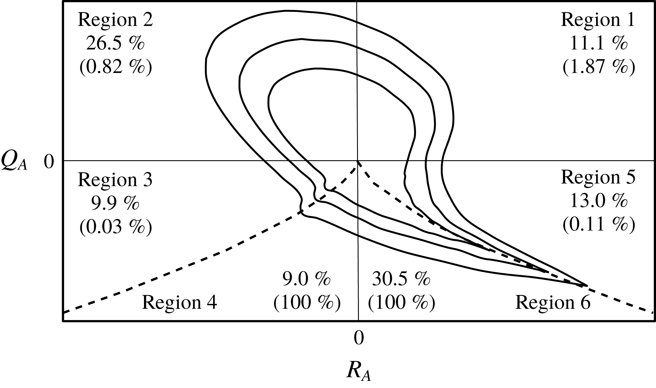
diagram showing contours for the typical joint distribution function, as well as the percentage occupancy of each region for the HIT numerical simulation and the efficiency of attaining the Lee bound (values in brackets). Thus, 1.87 % of occurrences in region 1 attain
 $\ell =1$
. The dashed line indicates the discriminant,
 $\unicode[STIX]{x1D6E5}=0$
, which defines the divide between regions 3 and 4, and 5 and 6, respectively. The Vieillefosse tail is depicted by the contours extending along the discriminant between regions 5 and 6.

To illustrate how efficient different regions in
 $Q_{A}-R_{A}$
space are at attaining the Lee bound, figure 1 is a sketch of the
 $Q_{A}-R_{A}$
diagram, with regions identified according to the typology adopted in our previous work (Keylock Reference Keylock2018):
(i) Region 1 –
$Q_{A}>0$
,
$R_{A}>0$
;(ii) Region 2 –
$Q_{A}>0$
,
$R_{A}<0$
;(iii) Region 3 –
$Q_{A}<0$
,
$\unicode[STIX]{x1D6E5}>0$
,
$R_{A}<0$
;(iv) Region 4 –
$Q_{A}<0$
,
$\unicode[STIX]{x1D6E5}<0$
,
$R_{A}<0$
;(v) Region 5 –
$Q_{A}<0$
,
$\unicode[STIX]{x1D6E5}>0$
,
$R_{A}>0$
;(vi) Region 6 –
$Q_{A}<0$
,
$\unicode[STIX]{x1D6E5}<0$
,
$R_{A}>0$
.


The dashed line in figure 1 is the discriminant,
 $\unicode[STIX]{x1D6E5}=0$
, and beneath it, corresponding to
 ${\sim}40\,\%$
of VGTs,
 $\ell =1$
is imposed by definition as discussed above. However, for
 $\unicode[STIX]{x1D6E5}>0$
the average occurrence over all regions is
 ${\sim}0.7\,\%$
of tensors, facilitated by
 $R_{A}>0$
and
 $Q_{A}>0$
. Thus, the net effect of the more efficient generation of
 $\ell =1$
states in region 1 is that regions 1 and 2 generate occurrences at the Lee bound at the same frequency as each other despite the 11.1 to 26.5 difference in relative frequency. In effect, this acts to induce a symmetry to the
 $Q_{A}-R_{A}$
diagram in the enstrophy-dominated regions if only the
 $\ell =1$
occurrences are considered. This potentially implies a relation between the
 $\ell =1$
occurrences and energetic flow structures as work using a triple decomposition into mean, coherent and fluctuating velocities, and extracting the coherent part using proper orthogonal decomposition, has found that the
 $Q_{A}-R_{A}$
diagram is approximately symmetric for the coherent part as shown in figure 6 of Buxton, Breda & Chen (Reference Buxton, Breda and Chen2017). We examine the relation between
 $\ell =1$
occurrences and coherent flow structures in greater detail below.
As shown in (2.11), the third invariant of the characteristic equation for the velocity gradient tensor,
 $R_{A}$
, may be decomposed into constituent strain production and enstrophy production terms,
 $-\text{det}(\unicode[STIX]{x1D64E}_{A})$
, and
 $\text{tr}(\unicode[STIX]{x03A9}_{A}^{2}\unicode[STIX]{x1D64E}_{A})$
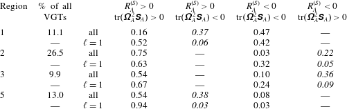
. Table 2 sub-divides the results for each region of the
 $Q_{A}-R_{A}$
diagram by the signs for these production terms, while also highlighting the differences that arise when
 $\ell =1$
. The region that is in strongest agreement with the results of Taylor (Reference Taylor1938b
) and Betchov (Reference Betchov1956) for the mean values is region 5, where 94 % of tensors had positive values for both strain production and enstrophy production. A similar magnitude of change is also seen for region 1, and the even clearer result is the near absence of cases where these terms are opposite in sign once
 $\ell =1$
.
Proportional occupancy of different regions of the
 $Q_{A}-R_{A}$
diagram as a function of region as well as strain production state and enstrophy production state. The sum of the values in each row of columns four to seven is 1.0. The second column therefore provides a means to weight the values in those columns to determine the proportional occupancy for all VGTs in HIT. The one value italicised in each row is the one possibility for the signs of
 $-\text{det}(\unicode[STIX]{x1D64E}_{B})$
and
 $\text{tr}(\unicode[STIX]{x03A9}_{B}^{2}\unicode[STIX]{x1D64E}_{B})$
for each region. Overall results are in the upper row for each region, and the results for
 $\ell =1$
are given beneath this.

To investigate this further, it is useful to expand the terms constituting
 $Q_{A}$
and
 $R_{A}$
to isolate the contributions from normal and non-normal terms. The second invariant of the VGT is traditionally written as stated in (2.10). Following Keylock (Reference Keylock2018) we may instead state that
 $$\begin{eqnarray}\displaystyle Q_{A}={\textstyle \frac{1}{2}}[(\Vert \unicode[STIX]{x03A9}_{B}\Vert ^{2}+\Vert \unicode[STIX]{x03A9}_{C}\Vert ^{2})-(\Vert \unicode[STIX]{x1D64E}_{B}\Vert ^{2}+\Vert \unicode[STIX]{x03A9}_{C}\Vert ^{2})], & & \displaystyle\end{eqnarray}$$
i.e.
 $Q_{A}=Q_{B}$
, where
 $$\begin{eqnarray}\displaystyle Q_{B}={\textstyle \frac{1}{2}}(\Vert \unicode[STIX]{x03A9}_{B}\Vert ^{2}-\Vert \unicode[STIX]{x1D64E}_{B}\Vert ^{2}), & & \displaystyle\end{eqnarray}$$
and the non-normal contribution cancels in the restricted Euler analysis. With regard to the production terms, we expand (2.11) as
 $$\begin{eqnarray}\displaystyle \left.\begin{array}{@{}c@{}}\displaystyle -\text{det}(\unicode[STIX]{x1D64E}_{A})=-\text{det}(\unicode[STIX]{x1D64E}_{B})-\text{det}(\unicode[STIX]{x1D64E}_{C})+\text{tr}(\unicode[STIX]{x03A9}_{C}^{2}\unicode[STIX]{x1D64E}_{B})\\ \displaystyle \text{tr}(\unicode[STIX]{x03A9}_{A}^{2}\unicode[STIX]{x1D64E}_{A})=\text{tr}(\unicode[STIX]{x03A9}_{B}^{2}\unicode[STIX]{x1D64E}_{B})-\text{det}(\unicode[STIX]{x1D64E}_{C})+\text{tr}(\unicode[STIX]{x03A9}_{C}^{2}\unicode[STIX]{x1D64E}_{B}).\end{array}\right\} & & \displaystyle\end{eqnarray}$$
The first term on the right-hand side of each equation in (3.3) is the normal term (strain production then enstrophy production), while the second and third terms have been termed the non-normal production and interaction production, respectively (Keylock Reference Keylock2018). The signs for the two normal terms in (3.3) are dictated by the sign for
 $R_{A}$
because
 $R_{A}=-\text{det}(\unicode[STIX]{x1D63C})=-\prod e_{i}$
, i.e.
 $$\begin{eqnarray}\displaystyle \left.\begin{array}{@{}c@{}}\text{sgn}[-\text{det}(\unicode[STIX]{x1D64E}_{B})]=\text{sgn}(R_{A})\\ \text{sgn}[\text{tr}(\unicode[STIX]{x03A9}_{B}^{2}\unicode[STIX]{x1D64E}_{B})]=-\text{sgn}(R_{A}).\end{array}\right\} & & \displaystyle\end{eqnarray}$$
The appropriate combination of these terms is italicised in each row of table 2 and it is clear that for HIT, only between 22 % and 38 % of cases retain the sign combination for
 $\unicode[STIX]{x1D63C}$
that is anticipated from the consideration of
 $\unicode[STIX]{x1D63D}$
. This highlights the importance of the non-normal and interaction terms from (3.3) for dictating the behaviour of
 $\unicode[STIX]{x1D63C}$
. For regions 1, 2 and 3, the most frequently occupied category has the same sign for enstrophy production, but a change in the sign for strain production relative to the italicised term. In contrast, for region 5, it is enstrophy production that changes sign. This is consistent with high strain production close to the Vieillefosse tail (Vieillefosse Reference Vieillefosse1984), which exists along
 $\unicode[STIX]{x1D6E5}=0$
for
 $R_{A}>0$
, i.e. between regions 5 and 6 in figure 1.
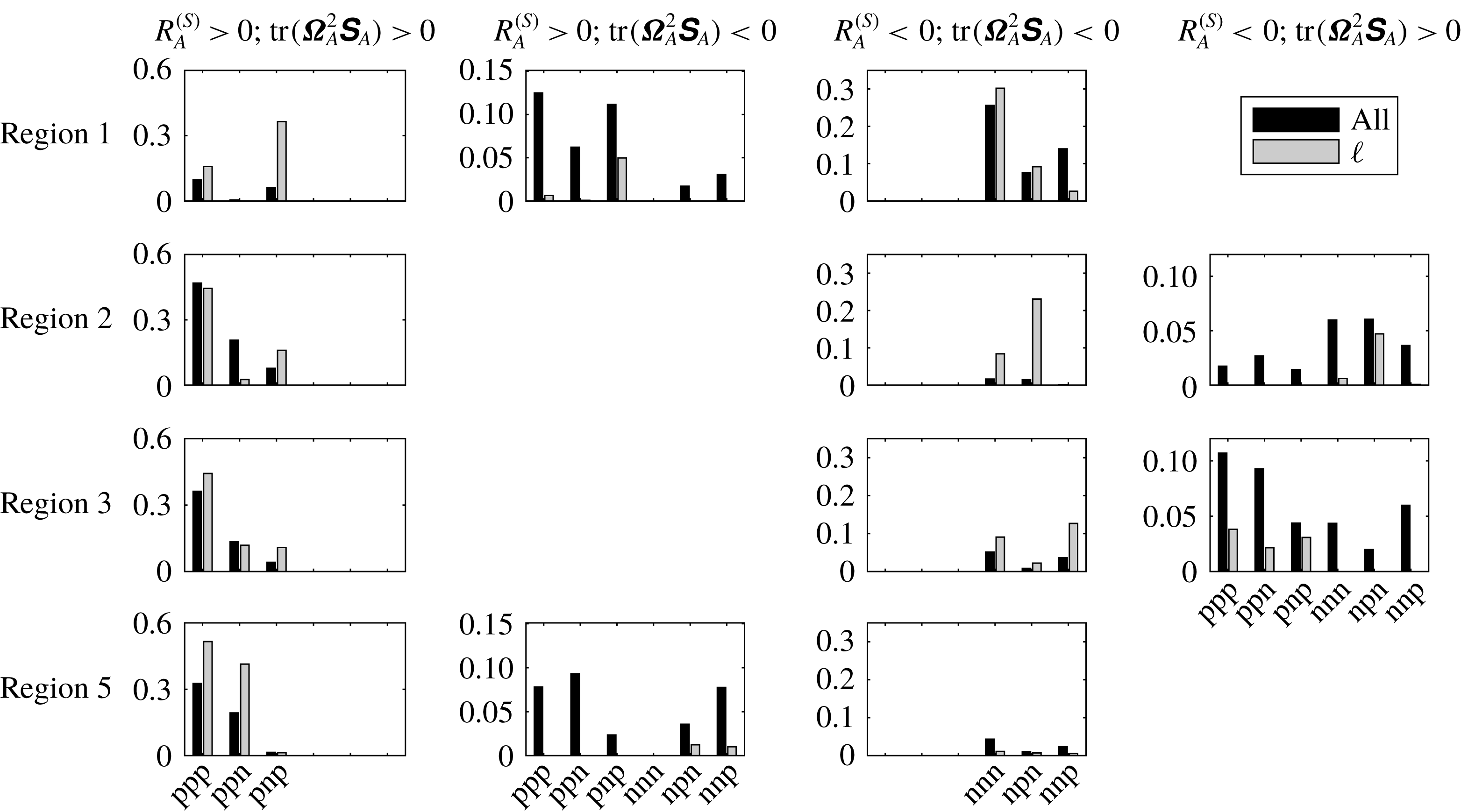
A partitioning of the results in table 2 by the values for the interaction production and non-normal production terms, and their sum. The abscissa for each panel indicates the possible sign combinations for these terms (‘p’
 $=$
positive, ‘n’
 $=$
negative). From left to right, each block of three characters gives the sign for
 $\text{tr}(\unicode[STIX]{x03A9}_{C}^{2}\unicode[STIX]{x1D64E}_{B})-\text{det}(\unicode[STIX]{x1D64E}_{C})$
,
 $\text{tr}(\unicode[STIX]{x03A9}_{C}^{2}\unicode[STIX]{x1D64E}_{B})$
and
 $-\text{det}(\unicode[STIX]{x1D64E}_{C})$
, respectively. The black bars are the results for all the data, while the light grey are the results for
 $\ell =1$
.

When examining the results for the
 $\ell =1$
regions in table 2, the effect of non-normality is very marked with only between 3 % and 9 % of cases retaining the sign combination anticipated based on the signs for
 $-\text{det}(\unicode[STIX]{x1D64E}_{B})$
and
 $\text{tr}(\unicode[STIX]{x03A9}_{B}^{2}\unicode[STIX]{x1D64E}_{B})$
. While one would expect a large effect of the non-normal contributions on the dynamics for the
 $\ell =1$
regions by definition, it is not necessarily the case that this would change the signs of
 $-\text{det}(\unicode[STIX]{x1D64E}_{A})$
and
 $\text{tr}(\unicode[STIX]{x03A9}_{A}^{2}\unicode[STIX]{x1D64E}_{A})$
because the non-normal and interaction production terms could act in a similar direction to the normal production terms. Instead, we find that between 52 % and 94 % of the VGTs in a given region with
 $\ell =1$
have positive values for both
 $-\text{det}(\unicode[STIX]{x1D64E}_{A})$
and
 $\text{tr}(\unicode[STIX]{x03A9}_{A}^{2}\unicode[STIX]{x1D64E}_{A})$
, with between 91 % and 97 % of cases having the same sign for these two production terms. This implies a pattern to the mutual alignment structure of the respective vorticity vectors and strain eigenvectors, which is examined further below.
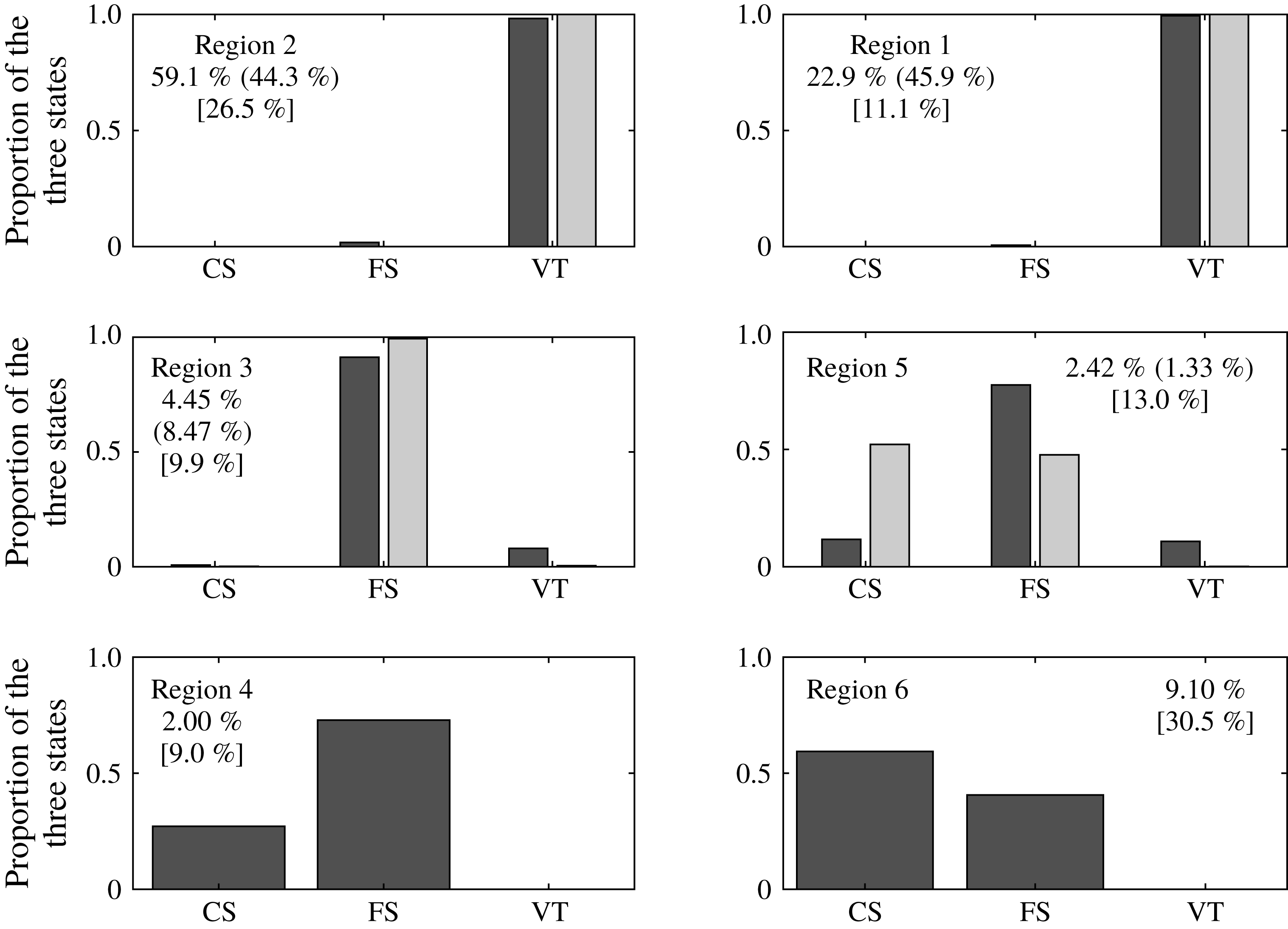
To understand in more detail how the terms in (3.3) lead to this result, we disaggregate each grouping from table 2 into the signs (‘p’ for positive, ‘n’ for negative) of the interaction production and non-normal production terms, and their sum in figure 2, where the black bars are the results for all VGTs and the light grey are for the
 $\ell =1$
cases. The terms are ordered such that the label ‘pnp’ on the abscissa means that the sum of interaction production and non-normal production is positive (first ‘p’), interaction production is negative, and non-normal production is positive (final ‘p’). The signs of the normal terms for each region are given in (3.4). Hence, in region 1, where normal strain production is already positive, the non-normal production and interaction production terms must counteract the sign for
 $\text{tr}(\unicode[STIX]{x03A9}_{B}^{2}\unicode[STIX]{x1D64E}_{B})$
in order to give a positive
 $\text{tr}(\unicode[STIX]{x03A9}_{A}^{2}\unicode[STIX]{x1D64E}_{A})$
. It is clear from the top-left panel of figure 2 that relative to all VGTs in region 1, the
 $\ell =1$
cases are particularly prone to have a negative interaction production and positive non-normal production, with the latter so great that not only is the sum of these two terms positive but
 $\text{tr}(\unicode[STIX]{x03A9}_{A}^{2}\unicode[STIX]{x1D64E}_{A})$
is also positive. As a consequence, the proportion of
 $\ell =1$
tensors in the top-left panel where
 $-\text{det}(\unicode[STIX]{x1D64E}_{A})>0$
and
 $\text{tr}(\unicode[STIX]{x03A9}_{A}^{2}\unicode[STIX]{x1D64E}_{A})>0$
is much greater than in the second panel where
 $-\text{det}(\unicode[STIX]{x1D64E}_{A})>0$
and
 $\text{tr}(\unicode[STIX]{x03A9}_{A}^{2}\unicode[STIX]{x1D64E}_{A})<0$
.
In region 2, there is a tendency for both
 $\text{tr}(\unicode[STIX]{x03A9}_{A}^{2}\unicode[STIX]{x1D64E}_{A})$
and
 $-\text{det}(\unicode[STIX]{x1D64E}_{A})$
to be positive for all cases, but this is focussed to a greater extent on the ‘ppp’ case, although there is still a relative excess for
 $\ell =1$
states in the ‘pnp’ category for
 $-\text{det}(\unicode[STIX]{x1D64E}_{A})>0$
and
 $\text{tr}(\unicode[STIX]{x03A9}_{A}^{2}\unicode[STIX]{x1D64E}_{A})>0$
seen in region 1. However, the mirror image of the result for region 1 also holds: a positive interaction production combines with negative non-normal production to give a negative sum, resulting in
 $\text{tr}(\unicode[STIX]{x03A9}_{A}^{2}\unicode[STIX]{x1D64E}_{A})<0$
; this arises largely at the expense of the probability of both constituents and their sum being negative, with
 $-\text{det}(\unicode[STIX]{x1D64E}_{A})<0$
and
 $\text{tr}(\unicode[STIX]{x03A9}_{A}^{2}\unicode[STIX]{x1D64E}_{A})>0$
. In regions 3 and 5, the dramatic decline in the probability that
 $-\text{det}(\unicode[STIX]{x1D64E}_{A})$
and
 $\text{tr}(\unicode[STIX]{x03A9}_{A}^{2}\unicode[STIX]{x1D64E}_{A})$
are opposite in sign is compensated by an increase for
 $\ell =1$
in the ‘ppp’ case for
 $-\text{det}(\unicode[STIX]{x1D64E}_{A})>0$
and
 $\text{tr}(\unicode[STIX]{x03A9}_{A}^{2}\unicode[STIX]{x1D64E}_{A})>0$
. The difference between these two regions is largely that in region 5,
 $\ell =1$
cases also exhibit a relative excess in the ‘ppn’ state for
 $-\text{det}(\unicode[STIX]{x1D64E}_{A})>0$
and
 $\text{tr}(\unicode[STIX]{x03A9}_{A}^{2}\unicode[STIX]{x1D64E}_{A})>0$
, implying that non-normal production is weak here. The related phenomenon in region 3 is the mirror image case where the ‘nnp’ state for
 $-\text{det}(\unicode[STIX]{x1D64E}_{A})<0$
and
 $\text{tr}(\unicode[STIX]{x03A9}_{A}^{2}\unicode[STIX]{x1D64E}_{A})<0$
becomes important.
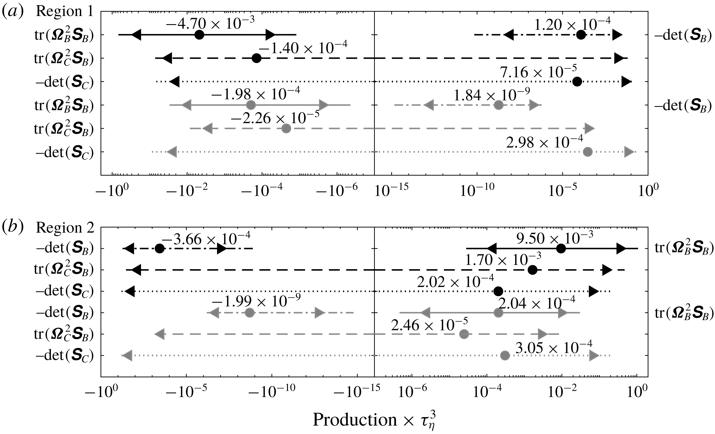
The range of observed values for the normal enstrophy production term (solid lines), normal strain production (dash-dotted lines), interaction production (dashed lines) and non-normal production (dotted lines) in region 1 (a) and region 2 (b). The black lines are for the full dataset and the grey are for the
 $\ell =1$
cases. All results are non-dimensionalised by
 $\unicode[STIX]{x1D70F}_{\unicode[STIX]{x1D702}}^{3}$
, and the lines extend from the 0.5 to the 99.5 percentile with the triangles at the 2.5 and 97.5 percentiles, and the median shown as a circle. The values for the medians are stated above each line.

3.3 The magnitudes of the constituent production terms
Moving away from an examination of the signs of the constituents, figure 3 shows boxplots of the values for the four production terms for region 1 (a) and region 2 (b) on logarithmically distributed axes. These were constructed for the negative and positive values separately and then re-combined, with values in grey those that attain the Lee bound. The signs of the normal enstrophy production and normal strain production are opposite for regions 1 and 2, which explains why they appear in different positions in the upper and lower panels. The typical magnitude of the normal enstrophy production is twice as great in region 2 (
 $9.50\times 10^{-3}$
) compared with region 1 (
 $-4.70\times 10^{-3}$
), while the median value for
 $|\text{det}(\unicode[STIX]{x1D64E}_{B})|$
is three times greater in region 2. Furthermore, the interaction production in the second row is twelve times greater in magnitude in region 2, with a sign difference for the median values, while non-normal production in the third row is 2.8 times greater, but positive on average in both regions.
When the flow attains the
 $\ell =1$
state (fourth to sixth rows in each panel), these differences in magnitude largely disappear. Values for the normal strain production are tiny, as expected, with those in region 2 only 8 % greater than for region 1. The equivalent percentage differences for normal enstrophy production, interaction production and non-normal production are 3 %, 9 % and 2 % respectively. There is also a clear change in the relative magnitude of the production terms in a given region for the
 $\ell =1$
states: normal strain production decreases from the third to the fourth term in magnitude, with non-normal production moving from fourth to the most important term. In this latter case, the median values increase by a factor of 4.2 in region 1 (from
 $7.16\times 10^{-5}$
to
 $2.98\times 10^{-4}$
) and by 50 % in region 2 (from
 $2.04\times 10^{-4}$
to
 $3.05\times 10^{-4}$
). While the median values for interaction production decrease for the
 $\ell =1$
states compared with all the remaining data, in region 1 this is by a factor of 6, compared with a factor of 69 in region 2. Similarly, values for normal enstrophy production decrease by a factor of 23.7 in region 1 and 46.6 in region 2.
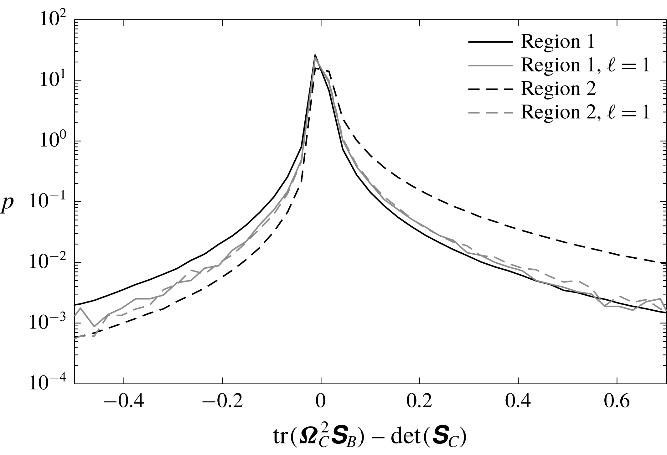
Probability density functions of the combined effect of the non-normal and interaction production terms in regions 1 (solid lines) and 2 (dashed lines). The black lines are for the full dataset and the grey are for the
 $\ell =1$
cases. All results are non-dimensionalised by
 $\unicode[STIX]{x1D70F}_{\unicode[STIX]{x1D702}}^{3}$
.

The above results suggest that region 1 is innately nearer the
 $\ell =1$
state compared with region 2 and probability density functions showing the impact of these changes on the combined production term,
 $\text{tr}(\unicode[STIX]{x03A9}_{C}^{2}\unicode[STIX]{x1D64E}_{B})-\text{det}(\unicode[STIX]{x1D64E}_{C})$
, are shown in figure 4, where the reduced smoothness of the grey lines (
 $\ell =1$
cases) is because fewer than 1 % of the overall cases are being sampled. This figure shows the overall consequences of the results in figure 3, where a typically positive non-normal production in both regions combines with an interaction production term with a median that changes sign following that for
 $\text{tr}(\unicode[STIX]{x03A9}_{B}^{2}\unicode[STIX]{x1D64E}_{B})$
. However, the difference declines greatly in magnitude for the
 $\ell =1$
cases. Thus, the explanation for why region 1 is more effective at generating
 $\ell =1$
states relative to region 2 is that the flow at the Lee bound has a particular and common probability distribution function for
 $\text{tr}(\unicode[STIX]{x03A9}_{C}^{2}\unicode[STIX]{x1D64E}_{B})-\text{det}(\unicode[STIX]{x1D64E}_{C})$
as seen in figure 4 and the flow in region 1 is typically nearer this state than that in region 2, particularly for positive values of
 $\text{tr}(\unicode[STIX]{x03A9}_{C}^{2}\unicode[STIX]{x1D64E}_{B})-\text{det}(\unicode[STIX]{x1D64E}_{C})$
. This result is useful as it implies that the two terms in (3.3) with contributions from
 $\unicode[STIX]{x1D63E}$
can be treated together for the purpose of understanding the development of
 $\ell =1$
states as the differences in interaction production seen in figure 3 are small enough in magnitude.
In summary the examination of the Eulerian properties of the
 $\ell =1$
occurrences show that they develop much more readily in region 1 where enstrophy exceeds total strain and the balance of strain production and enstrophy production is also positive. In this region it was shown in figure 2 that the key difference between
 $\ell =1$
instances and the flow in general was the relative excess of cases where both strain production and enstrophy production for
 $\boldsymbol{A}$
were positive, and the sum
 $\text{tr}(\unicode[STIX]{x03A9}_{C}^{2}\unicode[STIX]{x1D64E}_{B})-\text{det}(\unicode[STIX]{x1D64E}_{C})$
was also positive, but
 $\text{tr}(\unicode[STIX]{x03A9}_{C}^{2}\unicode[STIX]{x1D64E}_{B})$
was negative, meaning that
 $-\text{det}(\unicode[STIX]{x1D64E}_{C})$
must be large in magnitude. This is surprising in the sense that of the four production terms, this one is typically smallest in magnitude (Keylock Reference Keylock2018). Figure 3 shows that for both regions 1 and 2, when
 $\ell =1$
this non-normal production term is positive on average and larger in magnitude than the other terms. Figure 4 highlights that the nature of
 $\text{tr}(\unicode[STIX]{x03A9}_{C}^{2}\unicode[STIX]{x1D64E}_{B})-\text{det}(\unicode[STIX]{x1D64E}_{C})$
is similar in regions 1 and 2 when
 $\ell =1$
and this state is nearer the typical situation for region 1, explaining the difference in the relative frequency of attaining this flow state.
4 Lagrangian results
It is informative to undertake a Lagrangian analysis of the trajectories of fluid packets in HIT to determine how, and under what circumstances, the
 $\ell =1$
states arise. A total of
 $27^{3}$
fluid packets were tracked for
 $240\unicode[STIX]{x1D70F}_{\unicode[STIX]{x1D702}}$
at a temporal sampling interval of
 $0.05\unicode[STIX]{x1D70F}_{\unicode[STIX]{x1D702}}$
, with each packet initially spaced
 $2\unicode[STIX]{x1D706}$
from its neighbours to establish an initial spatial independence between samples. The domain size was
 ${\sim}(56\unicode[STIX]{x1D706})^{3}$
so 27 samples could be realised between
 $\unicode[STIX]{x1D706}$
and
 $2\unicode[STIX]{x03C0}-\unicode[STIX]{x1D706}$
in each direction. In total, 335 000
 $\ell =1$
events occurred with a duration ranging from
 $0.05<\unicode[STIX]{x1D70F}_{\unicode[STIX]{x1D702}}<3.25$
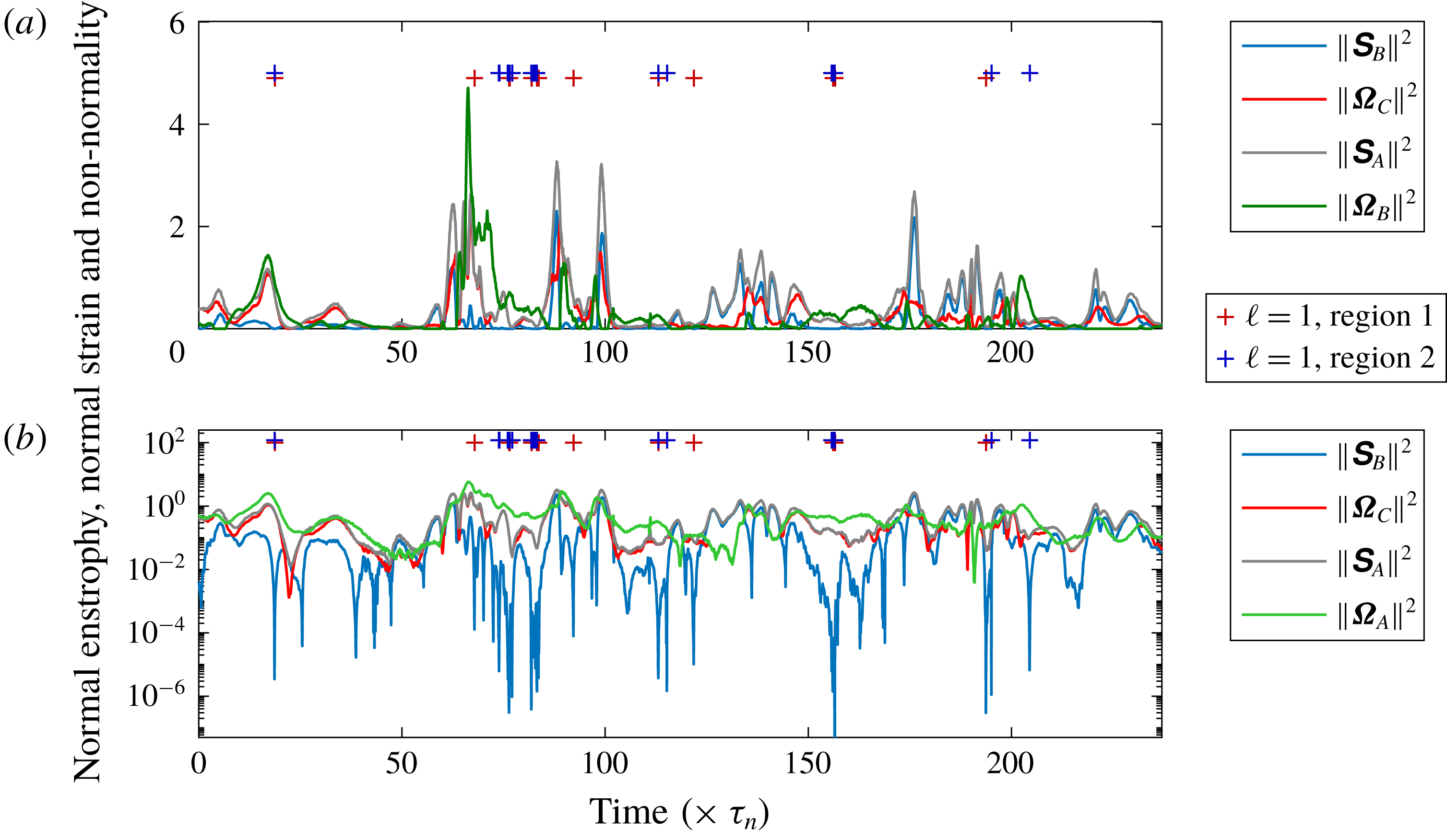
. The example Lagrangian trace shown in figure 5 had 51 individual
 $\ell =1$
occurrences, with 22 arising in region 1, 28 in region 2 and one in region 3. Altogether, there are 197 changes in region of the
 $Q_{A}-R_{A}$
diagram for this trace, with a median duration in a region of
 $0.5\unicode[STIX]{x1D70F}_{\unicode[STIX]{x1D702}}$
, and a 95th percentile of
 $4.3\unicode[STIX]{x1D70F}_{\unicode[STIX]{x1D702}}$
. The sign for
 $Q_{A}$
may be discerned in panel (a) by the difference between the green and blue traces, and in panel (b) by the green and grey traces. Panel (a) highlights some intensive and intermittent dissipative events where the normal enstrophy is very small or zero at
 $t\approx 100\unicode[STIX]{x1D70F}_{\unicode[STIX]{x1D702}}$
and
 $t\approx 175\unicode[STIX]{x1D70F}_{\unicode[STIX]{x1D702}}$
, as well as an occurrence at
 $t\approx 90\unicode[STIX]{x1D70F}_{\unicode[STIX]{x1D702}}$
, where normal enstrophy is less than normal strain but significantly non-zero. This forms the tail end of a
 ${\approx}40\unicode[STIX]{x1D70F}_{\unicode[STIX]{x1D702}}$
duration period where normal enstrophy is heightened, and the trajectory moves between regions 1 and 2 exclusively for the first 22.4
 $\unicode[STIX]{x1D70F}_{\unicode[STIX]{x1D702}}$
of this period (from
 $t=63.5\unicode[STIX]{x1D70F}_{\unicode[STIX]{x1D702}}$
to
 $t=85.9\unicode[STIX]{x1D70F}_{\unicode[STIX]{x1D702}}$
). Panel (b) shows that the values for normal straining are very low for these times as the trajectory passes through a region that can be legitimately termed a coherent flow structure in the sense that normal enstrophy is orders of magnitude greater than normal straining. The low normal straining drives the flow towards the
 $\ell =1$
state and twenty three of the 51
 $\ell =1$
occurrences arise in this 22.4
 $\unicode[STIX]{x1D70F}_{\unicode[STIX]{x1D702}}$
window.
An illustration of one of the
 $27^{3}$
Lagrangian paths followed for a duration of
 $240\unicode[STIX]{x1D70F}_{\unicode[STIX]{x1D702}}$
shown on a linear ordinate (a) and a logarithmic ordinate (b). The red and blue crosses show the occurrences where
 $\ell =1$
for regions 1 and 2, respectively, with the region 2 crosses displaced slightly above those for region 1. Because
 $\Vert \unicode[STIX]{x03A9}_{B}\Vert ^{2}=0$
in regions 4 and 6, these data are only plotted in panel (a), with
 $\Vert \unicode[STIX]{x03A9}_{A}\Vert ^{2}$
shown instead in panel (b).

4.1 Lagrangian trajectories and durations for the
$\ell =1$
states

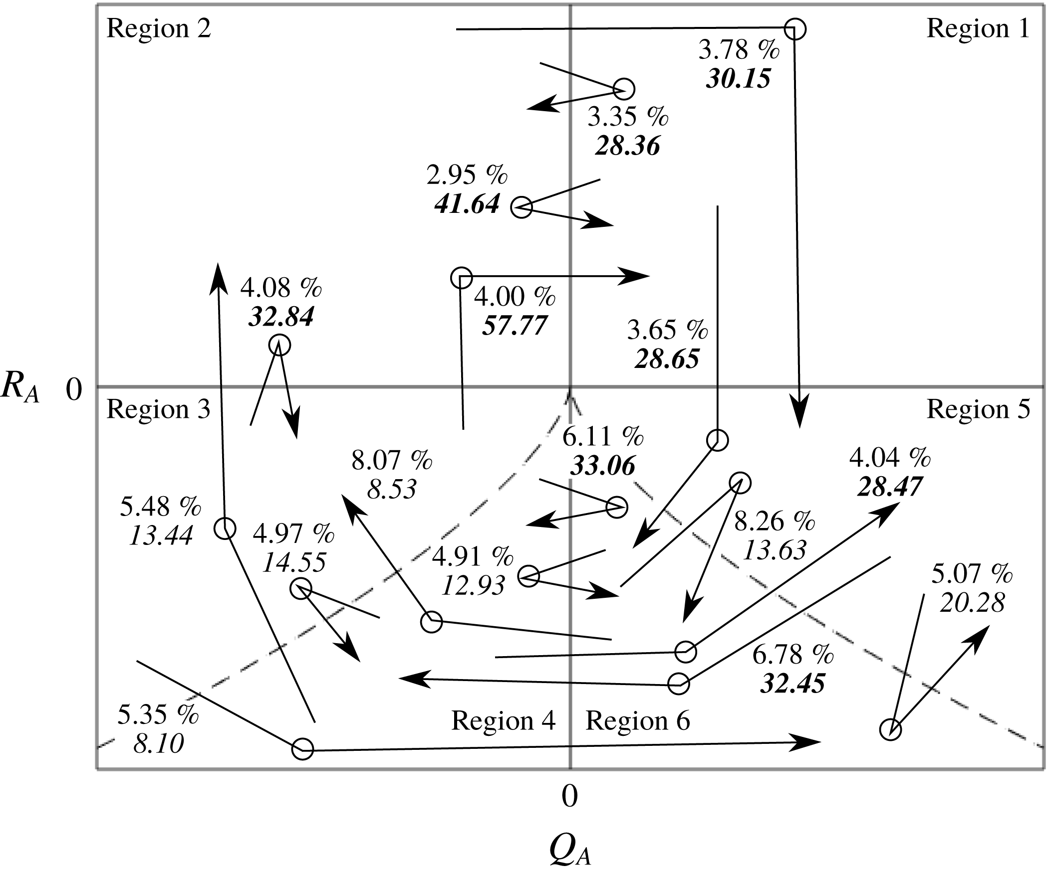
Figure 6 is a sketch of sixteen Lagrangian trajectory segments, each of which exhibits a change in region in
 $Q_{A}-R_{A}$
space. The arrow shown passes from the region of origin to termination for the chosen trajectory, and the circle half-way along the arrow is the intermediate region where the flow primarily resides while on such a trajectory. All told these sixteen cases accounted for 80.85 % of the total number of trajectories that crossed into different regions. For each case, the mean time spent in the region denoted by the circle is given in italics and this is in bold if it exceeds
 $25\unicode[STIX]{x1D70F}_{\unicode[STIX]{x1D702}}$
. The well-known average clockwise trajectory through regions of the
 $Q_{A}-R_{A}$
diagram (Lüthi et al.
Reference Lüthi, Holzner and Tsinober2009) is discerned visually. It is also the case that when the trajectories are in the upper part of the diagram (regions 1 and 2) they are relatively persistent with mean durations in these two regions ranging from
 $28\leqslant \unicode[STIX]{x1D70F}_{\unicode[STIX]{x1D702}}<58$
. This may be contrasted with regions 3–6 which account for eleven of the sixteen trajectories and 78 % of the illustrated occurrences, but with a typically reduced duration (an average duration of
 $\langle \unicode[STIX]{x1D70F}_{\unicode[STIX]{x1D702}}\rangle =18.8$
when weighted by the percentage of occurrences, compared with
 $\langle \unicode[STIX]{x1D70F}_{\unicode[STIX]{x1D702}}\rangle =38.4$
in regions 1 and 2).
A sketch of the
 $Q_{A}-R_{A}$
diagram with sixteen trajectories superimposed that accounted for over 80 % of recorded trajectories that passed through one of the six regions of
 $Q_{A}-R_{A}$
space. In each case, the circle indicates the region where the trajectory resided, with the region from which it originated
 ${\leqslant}0.05\unicode[STIX]{x1D70F}_{\unicode[STIX]{x1D702}}$
before the primary region shown by the tail of the arrow, and that
 ${\leqslant}0.05\unicode[STIX]{x1D70F}$
after it left the primary region shown by the head of the arrow. The label next to each arrow shows the percentage of recorded trajectories associated with this configuration, while the number in italics is the mean time spent in the primary region (in multiples of
 $\unicode[STIX]{x1D70F}_{\unicode[STIX]{x1D702}}$
). The bold cases are those where this duration exceeded
 $25\unicode[STIX]{x1D70F}_{\unicode[STIX]{x1D702}}$
. The absence of values on the axes is to indicate that the locations of each trajectory are for illustrative purposes.

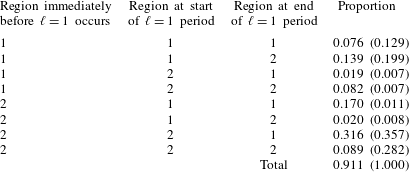
The manner in which the
 $\ell =1$
state is attained in the positive
 $Q_{A}$
part of the
 $Q_{A}-R_{A}$
diagram (corresponding to 91.1 % of cases). The proportions in brackets give the relative frequency of Lagrangian trajectories that attain the
 $\ell =1$
state for a duration greater than
 $0.4\unicode[STIX]{x1D70F}_{\unicode[STIX]{x1D702}}$
, which is the case for just 0.93 % of cases.

On average, each of the
 $27^{3}$
Lagrangian trajectories attained the
 $\ell =1$
state for 0.66 % of its duration (for the example trajectory in figure 5 the rate is some three times higher than this). As is shown in the bottom row of table 3, some 91 % of
 $\ell =1$
occurrences were solely in regions 1 and 2. This table shows the eight possible permutations for these two regions. All other cases, which involved regions 3 and 5 in some way, were less frequent than any of the listed eight states. About a third of the occurrences are for trajectories already in region 2 that commenced the
 $\ell =1$
state in region 2 and ended in region 1. A closely related case where the transition from region 2 to region 1 arose right at the commencement of the
 $\ell =1$
state (second row), accounted for a further
 $0.17/0.91=19\,\%$
of cases. However, the next most common occurrence was associated with a movement counter to that anticipated from the clockwise restricted Euler solution (region 1 to region 2 change representing 0.139/0.91 = 15 % of cases). Two of the eight cases identify changes from
 $\ell =0$
to
 $\ell =1$
while remaining in a given region. These highlight the utility of the decomposition into normal and non-normal contributions to the production budget for explaining this dynamics. A transition from region 2 to region 1 (or vice versa) means that
 $R_{A}$
has changed sign, demarcating a change in the interplay between enstrophy production and strain production. The cases in the first and last rows cannot be identified based on sign changes for the classic terms.
4.2 The Lee bound and the sign of
$R_{A}$

Directly related to the above discussion, there are four possible ways for the third invariant of the characteristic equation for the VGT to be zero, two of which are immediately apparent from a conventional analysis: either
 $-\text{det}(\unicode[STIX]{x1D64E}_{A})=\text{tr}(\unicode[STIX]{x03A9}_{A}^{2}\unicode[STIX]{x1D64E}_{A})$
, or
 $\Vert \unicode[STIX]{x1D64E}_{A}\Vert \rightarrow 0$
. In addition, however, we may use (3.3) to note that two alternatives are that either the normal strain production and normal enstrophy production are in balance, or
 $\Vert \unicode[STIX]{x1D64E}_{B}\Vert \rightarrow 0$
. An inspection of (2.17) shows that the latter mechanism is the simplest way to obtain
 $\ell =1$
: a dramatic decline in normal strain production with the non-normal production unaffected and greater in magnitude than interaction production results in
 $\Vert \unicode[STIX]{x1D649}\Vert$
remaining approximately constant, with
 $\Vert \unicode[STIX]{x1D64E}_{B}\Vert \rightarrow 0$
meaning that
 $\sqrt{2}\Vert \unicode[STIX]{x1D64E}_{A}\Vert \rightarrow \Vert \unicode[STIX]{x1D649}\Vert$
leads to
 $\ell =1$
. In contrast, if the normal enstrophy production and normal strain production terms are in balance, this does not necessarily lead to
 $\ell =1$
because of a potentially significant contribution to
 $\sqrt{2}\Vert \unicode[STIX]{x1D64E}_{A}\Vert$
from
 $\Vert \unicode[STIX]{x1D64E}_{B}\Vert$
. It is more straightforward for
 $\Vert \unicode[STIX]{x1D64E}_{B}\Vert \rightarrow 0$
than
 $\Vert \unicode[STIX]{x1D64E}_{A}\Vert \rightarrow 0$
as the latter requires both the normal and non-normal components of the strain to tend to zero.
This conclusion is supported by the statement in table 3 that only 0.93 % of the
 $\ell =1$
states persist for longer than
 $0.4\unicode[STIX]{x1D70F}_{\unicode[STIX]{x1D702}}$
in the Lagrangian frame, implying that the phenomenon is driven by the behaviour of the local terms rather than the more spatially extensive contributions from the non-local part of the pressure Hessian, which are expected to persist for a longer duration, related more closely to the duration of a flow structure rather than a fraction of the Kolmogorov time. In addition, because the first and last rows of table 3 show that in 16.5 % of instances the
 $\ell =1$
state is attained without a change in region, this must mean that the impact of the decline in normal straining on
 $-\text{det}(\unicode[STIX]{x1D64E}_{B})$
is so much greater than
 $\text{tr}(\unicode[STIX]{x03A9}_{B}^{2}\unicode[STIX]{x1D64E}_{B})$
that the sign of
 $R_{A}$
is unaffected, a situation that arises either as a consequence of large normal enstrophy or limited alignment between
 $\unicode[STIX]{x1D74E}_{B}$
and the eigenvectors for
 $\unicode[STIX]{x1D64E}_{B}$
.
Assuming that there are no systematic differences in the strength of alignment between
 $\unicode[STIX]{x1D74E}_{C}$
and the eigenvectors for
 $\unicode[STIX]{x1D64E}_{B}$
relative to between
 $\unicode[STIX]{x1D74E}_{B}$
and the eigenvectors for
 $\unicode[STIX]{x1D64E}_{B}$
, then a decline in
 $\Vert \unicode[STIX]{x1D64E}_{B}\Vert$
will impact the interaction production term to a similar degree as the normal enstrophy production. It was noted with reference to figure 3 that the non-normal production term is the greatest in magnitude of the four production terms where
 $\ell =1$
. As a consequence, to establish if the mechanism driving these changes is driven by the magnitudes of the terms or their alignments, it is important to examine the mutual alignments of
 $\unicode[STIX]{x1D74E}_{B}$
with the eigenvectors for
 $\unicode[STIX]{x1D64E}_{B}$
, denoted by
 $\unicode[STIX]{x1D65A}_{i}^{(B)}$
and ordered with regards to the eigenvalues placed in descending order, and those between
 $\unicode[STIX]{x1D74E}_{C}$
and
 $\unicode[STIX]{x1D65A}_{i}^{(B)}$
.
4.3 Alignment structure of the vorticity components and the normal straining
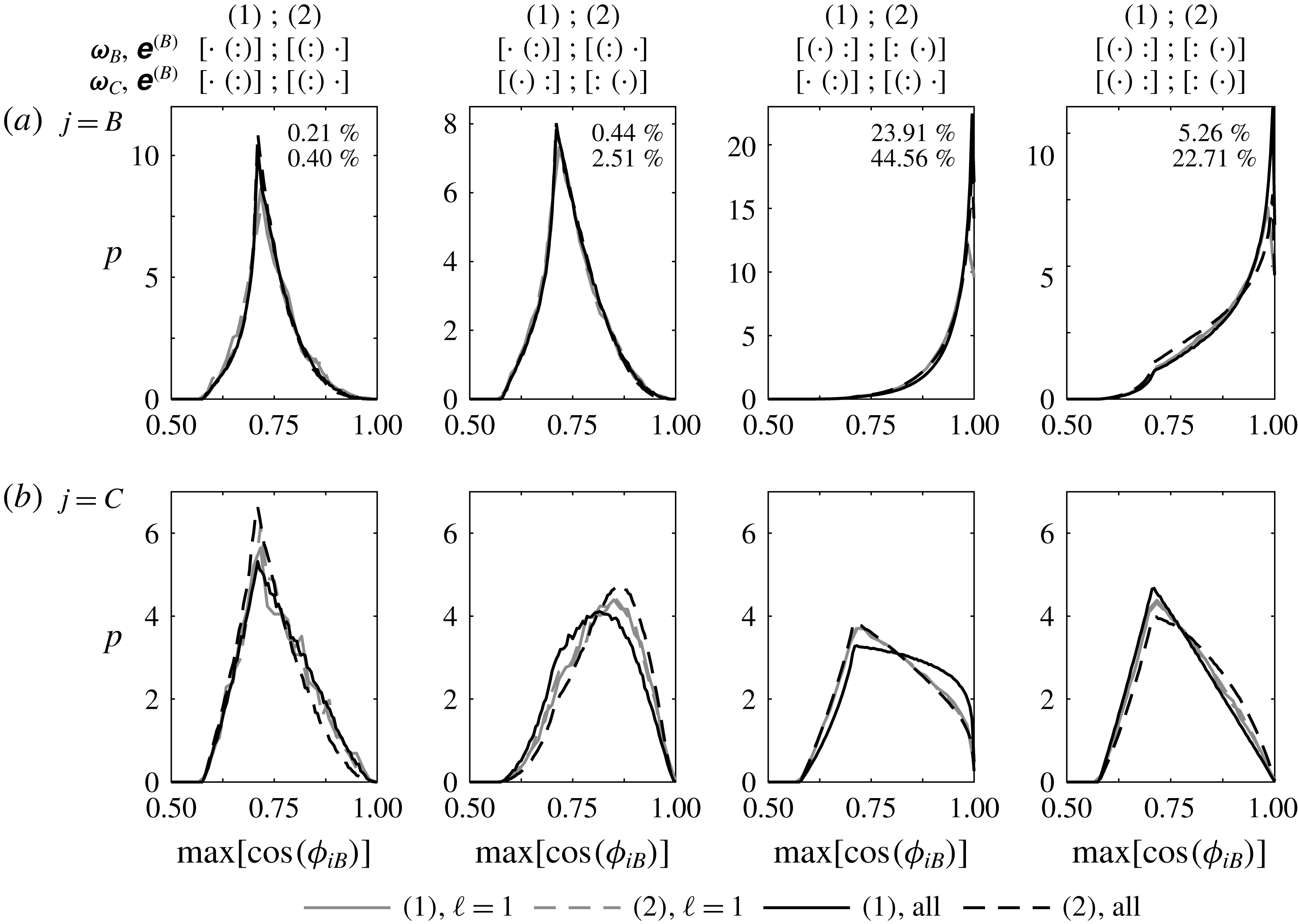
Probability density functions of the maximum alignment between the vorticity vectors,
 $\unicode[STIX]{x1D74E}_{B}$
(a) and
 $\unicode[STIX]{x1D74E}_{C}$
(b) and the eigenvectors of the normal strain tensor,
 $\unicode[STIX]{x1D65A}_{i}^{(B)}$
, for regions 1 and 2 of the
 $Q_{A}-R_{A}$
diagram. The eigenvalues of
 $\unicode[STIX]{x1D64E}_{B}$
placed in descending rank order are such that either
 $\unicode[STIX]{x1D65A}_{3}^{(B)}=-2\unicode[STIX]{x1D65A}_{1}^{(B)}=-2\unicode[STIX]{x1D65A}_{2}^{(B)}$
(region 1) or
 $\unicode[STIX]{x1D65A}_{1}^{(B)}=-2\unicode[STIX]{x1D65A}_{2}^{(B)}=-2\unicode[STIX]{x1D65A}_{3}^{(B)}$
(region 2), where the former is a rod-like flow structure and the latter is disc-like. Graphically, these are indicated above each panel as
 $[\cdot ~:]$
and
 $[:~\cdot ]$
, respectively and results for both regions are shown in each of the eight panels, with the solid lines the results for region 1 and the dashed lines those for region 2 (region numbers are given in brackets in the legend; results at the Lee bound are shown in grey). The four columns of panels segregate which strain eigenvector the vorticity vectors are most aligned with for both
 $\unicode[STIX]{x1D74E}_{B}$
and
 $\unicode[STIX]{x1D74E}_{C}$
. This is indicated by the round brackets in the eigenvalue arrangements. Thus, in the second column, and for region 1, we have
 $[\cdot ~(:)]$
for
 $\max [\cos (\unicode[STIX]{x1D719}_{B,B})]$
, the strongest alignment between
 $\unicode[STIX]{x1D74E}_{B}$
and the
 $\unicode[STIX]{x1D65A}^{(B)}$
, and
 $[(\cdot )~:]$
for
 $\max [\cos (\unicode[STIX]{x1D719}_{C,B})]$
. Hence, in this column, in region 1 the normal vorticity vector is most aligned with one of the two equal and positive eigenvalues, while the non-normal vorticity vector is most aligned with the only negative eigenvalue. The two percentage values give the relative proportion of all the results shown in each panel for regions 1 (upper value) and 2 (lower value). I.e. over 68 % of the tensors have the alignment properties given by the third column.

Denoting the vorticity–strain alignments by
 $\unicode[STIX]{x1D719}_{j,B}$
where
 $j\in \{B,C\}$
denotes the relevant vorticity vector, then histograms of the values for
 $\max [\cos (\unicode[STIX]{x1D719}_{j,B})]$
are given in figure 7, where the maximum is taken over the eigenvectors. The top row of panels show results for
 $\max [\cos (\unicode[STIX]{x1D719}_{B,B})]$
and the bottom row for
 $\max [\cos (\unicode[STIX]{x1D719}_{C,B})]$
. In each panel, results are shown for both regions 1 (solid lines) and region 2 (dashed lines), which necessarily have an opposite configuration for the eigenvalues of
 $\unicode[STIX]{x1D64E}_{B}$
:
 $\unicode[STIX]{x1D65A}_{3}^{(B)}=-2\unicode[STIX]{x1D65A}_{1}^{(B)}=-2\unicode[STIX]{x1D65A}_{2}^{(B)}$
(region 1) or
 $\unicode[STIX]{x1D65A}_{1}^{(B)}=-2\unicode[STIX]{x1D65A}_{2}^{(B)}=-2\unicode[STIX]{x1D65A}_{3}^{(B)}$
(region 2). These eigenvalues are the real part of those for
 $\unicode[STIX]{x1D63D}$
, which form a conjugate pair and a real value. Hence, we represent the eigenvalues for
 $\unicode[STIX]{x1D64E}_{B}$
pictorially as
 $[\cdot ~:]$
for region 1 and
 $[:~\cdot ]$
for region 2, respectively. There are then four possibilities for which eigenvector of
 $\unicode[STIX]{x1D64E}_{B}$
exhibits the greatest alignment: either the eigenvector for the single eigenvalue or for one of the pair of eigenvalues, with this criterion applying to both
 $\max [\cos (\unicode[STIX]{x1D719}_{B,B})]$
and
 $\max [\cos (\unicode[STIX]{x1D719}_{C,B})]$
. These four states are delimited by the columns in figure 7, where the rounded bracket indicates the eigenvalue corresponding to the most aligned eigenvector. The percentages in each upper panel show the relative frequency of each of these possibilities, with the first stated value that for region 1, and the lower value for region 2. It is clear that the most important is the third column where
 $\max [\cos (\unicode[STIX]{x1D719}_{B,B})]$
is for the eigenvector corresponding to the single eigenvalue of
 $\unicode[STIX]{x1D64E}_{B}$
, e.g.
 $[(\cdot )~:]$
and
 $\max [\cos (\unicode[STIX]{x1D719}_{C,B})]$
for an eigenvector corresponding to one of the paired eigenvalues, e.g.
 $[\cdot ~(:)]$
. This makes up 68 % of cases, and is particularly dominant for region 1 (80 % of the 29.8 % of occurrences in region 1). While the results in columns 1 and 3 have about double the likelihood for region 2 compared with region 1, the occurrences in columns 2 and 4 are four to five times more likely in region 2, highlighting a clear difference in the alignment behaviour for the non-normal component of the vorticity.
While the results in figure 7 show that the distribution functions are similar for the
 $\ell =1$
states compared with the full dataset, it is not clear if the stated percentages also apply to the
 $\ell =1$
states. Consequently, table 4 presents the same results but classified by
 $\ell$
. There is a remarkable similarity in the results at the Lee bound irrespective of whether the flow is in region 1 or 2. For example, for
 $\ell =1$
, 70 % of results have the configuration given by the third column, while this varies between 63 % and 80 % for regions 1 and 2 when
 $\ell =0$
. Given that the third and fourth columns have the same alignment structure for
 $\max [\cos (\unicode[STIX]{x1D719}_{B,B})]$
(an alignment with the eigenvector for the single eigenvalue), the change in alignment structure for
 $\max [\cos (\unicode[STIX]{x1D719}_{C,B})]$
from one where the alignment is with the eigenvector for the single eigenvalue (column 4) to one where it is with the pair (column 3) results in an increase in the relative frequency by a factor of 2.6 for the
 $\ell =1$
states compared with 4.6 for
 $\ell =0$
in region 1 and 2.0 for
 $\ell =0$
in region 2.
The percentage of occurrences of different vorticity–strain alignment states for regions 1 and 2 of the
 $Q_{A}-R_{A}$
diagram, adopting the same notation as used in figure 7, and isolating the results for
 $\ell =0$
and
 $\ell =1$
.

Given the similarity in the relative frequency of the
 $\ell =1$
cases between regions 1 and 2, the results in figure 7 for the
 $\ell =1$
cases (grey lines) can be considered directly, without any need to weight the density functions by frequency. It is clear that the distributions for
 $\max [\cos (\unicode[STIX]{x1D719}_{B,B})]$
have a very similar behaviour in each panel irrespective of if one is considering regions 1 or 2, or
 $\ell \in \{0,1\}$
. It is also intuitive that there is a tendency to perfect alignment in the third and fourth columns where
 $\max [\cos (\unicode[STIX]{x1D719}_{B,B})]$
involves the single eigenvalue, and
 $\cos (\unicode[STIX]{x03C0}/4)=\sqrt{2}/2$
in the first and second columns where it involves the pair. Based on these results, one might anticipate
 $\max [\cos (\unicode[STIX]{x1D719}_{C,B})]\rightarrow 1$
in the second and fourth columns where the alignment is with the single eigenvalue, but only in the former case does the mode for the distributions depart from
 $\sqrt{2}/2$
. Indeed, it is the results for region 1 for all data (solid line) in the third column where there is the greatest tendency for
 $\max [\cos (\unicode[STIX]{x1D719}_{C,B})]\rightarrow 1$
, but the alignment here is with one of the pair of eigenvalues. In this panel (the bottom panel in the third column), the results for
 $\ell =1$
in both regions follow those for region 2. In the other panels in the bottom row, the two density functions for
 $\ell =1$
are superimposed nearly perfectly and lie in between the results for regions 1 and 2 for all data. This superposition of the alignment histograms for
 $\ell =1$
in regions 1 and 2, and the similar relative frequencies in table 4, mean that one can go further than the results in figure 4. The
 $\ell =1$
state is not only similar across regions 1 and 2 in terms of the sum of the interaction production and non-normal production terms, it is also similar in terms of the alignment structures underpinning these two terms – there is a universal characteristic to the
 $\ell =1$
state in vortical regions. Furthermore, the broad similarity in the alignment distributions means that the differences in the average values for the terms examined in figure 3 between the
 $\ell =0$
and
 $\ell =1$
states are because of the dramatic decline in
 $\Vert \unicode[STIX]{x1D64E}_{B}\Vert$
, rather than because of alignment differences.
4.4 Changes in the contributing terms as
$\ell =1$
is attained

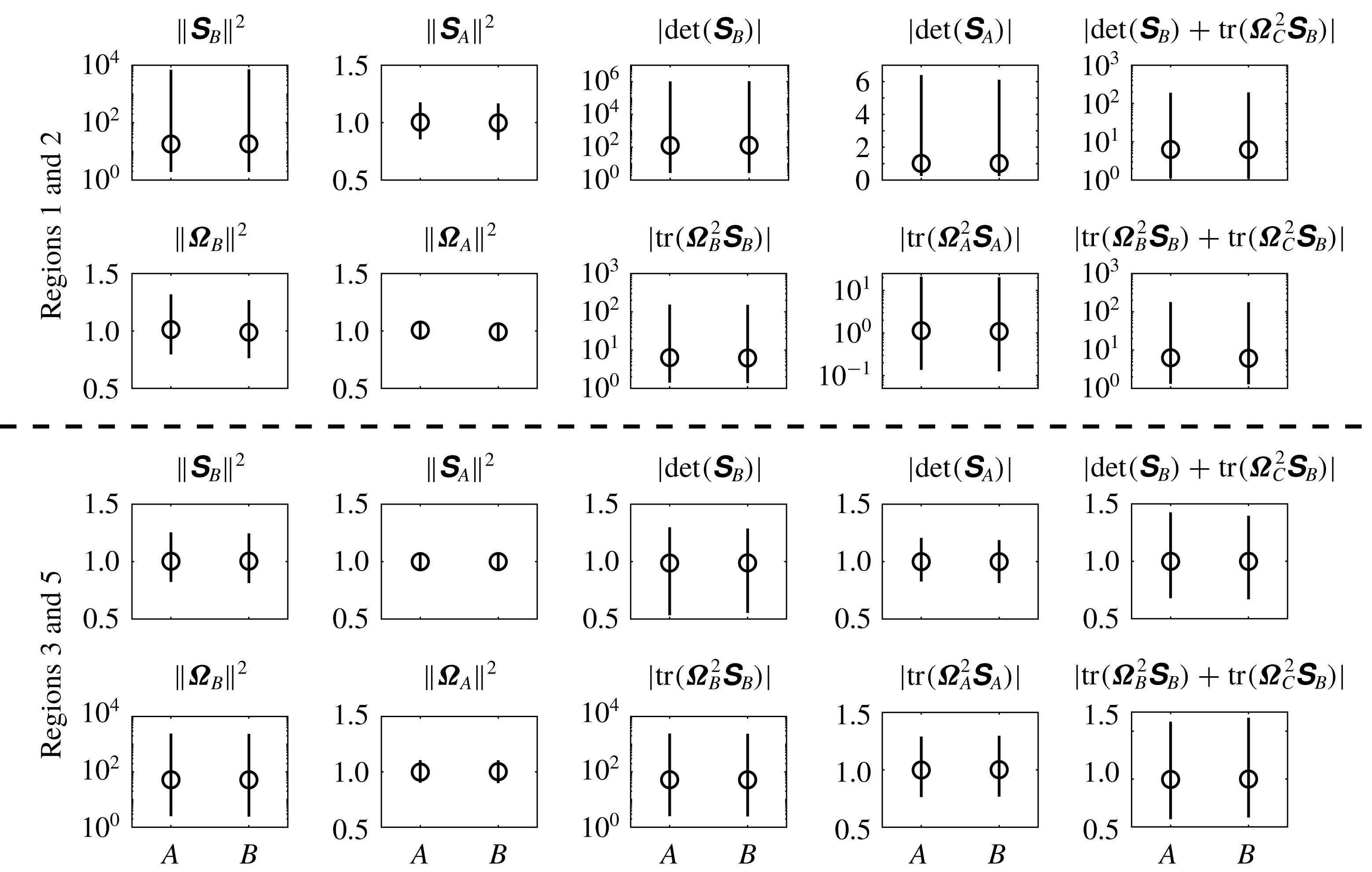
Median values (circles) for the magnitude of the ratio of the term stated above each panel between the flow immediately before the
 $\ell =1$
state to the mean during that state (A on the abscissa) and the ratio between the flow immediately after the
 $\ell =1$
state to the mean during that state (B on the abscissa). The top group of ten panels show results from regions 1 and 2, while the lower group are for regions 3 and 5. In each set, the upper row pertains to total strain, strain production and its constituents, while the lower is to enstrophy, enstrophy production and its constituents. The lines in each panel provide the range of values between the 2.5 % and 97.5 % quantiles.

The results in figure 8 show how the attainment of the Lee bound and the associated decline of the magnitude of the local terms impact the magnitude of the classical terms:
 $\Vert \unicode[STIX]{x1D64E}_{A}\Vert ^{2}$
,
 $\Vert \unicode[STIX]{x03A9}_{A}\Vert ^{2}$
,
 $-\text{det}(\unicode[STIX]{x1D64E}_{A})$
and
 $\text{tr}(\unicode[STIX]{x03A9}_{A}^{2}\unicode[STIX]{x1D64E}_{A})$
. In every panel in this figure, the very similar nature of the results for ‘A’ and ‘B’ indicate that there is not, on average, any significant, preferred trend for the evolution of these terms over the duration of the
 $\ell =1$
state as the ratios of the values for the before and after
 $\ell =1$
states to those during the
 $\ell =1$
state are similar. Considering regions 3 and 5 first (the bottom group of ten panels), it is clear that the ratios for all the strain-related terms are centred at 1.0; there is no observable impact of the attainment of the bound on the local or traditional terms, as anticipated because the bound in these regions is given by the rotation rate as described in (2.17). Attainment of the bound results in a typical decline in the magnitudes for both
 $\Vert \unicode[STIX]{x03A9}_{B}\Vert ^{2}$
and
 $\text{tr}(\unicode[STIX]{x03A9}_{B}^{2}\unicode[STIX]{x1D64E}_{B})$
by a factor of
 ${\sim}52$
. However, this dramatic effect has no noticeable impact on the magnitudes for
 $\Vert \unicode[STIX]{x03A9}_{A}\Vert ^{2}$
or
 $\text{tr}(\unicode[STIX]{x03A9}_{A}^{2}\unicode[STIX]{x1D64E}_{A})$
, with values remaining very close to 1.0. Given that there are three terms on the right-hand side of (3.3), that the change in
 $|\text{tr}(\unicode[STIX]{x03A9}_{B}^{2}\unicode[STIX]{x1D64E}_{B})|$
is not reflected in
 $|\text{tr}(\unicode[STIX]{x03A9}_{A}^{2}\unicode[STIX]{x1D64E}_{A})|$
could, in principle, be a consequence of the interaction production term or the non-normal production term. The right-most panel on the bottom row of figure 8 demonstrates that the inclusion of the interaction production term is sufficient to return the ratio to 1.0, i.e. there is no significant effect of non-normal production on average in this case.
In contrast, the equivalent panel for the results for regions 1 and 2 has a median value of
 $|\text{tr}(\unicode[STIX]{x03A9}_{B}^{2}\unicode[STIX]{x1D64E}_{B})+\text{tr}(\unicode[STIX]{x03A9}_{C}^{2}\unicode[STIX]{x1D64E}_{B})|=6.2$
. With the median for
 $|\text{tr}(\unicode[STIX]{x03A9}_{B}^{2}\unicode[STIX]{x1D64E}_{B})|$
of the order of 1.0, interaction production must be lower in magnitude when
 $\ell =1$
to drive the median towards 6.2, and non-normal production must be greater in magnitude when
 $\ell =1$
such that the median for
 $|\text{tr}(\unicode[STIX]{x03A9}_{A}^{2}\unicode[STIX]{x1D64E}_{A})|$
is similar to 1. This evidence for the importance of the non-normal production agrees with the results in figure 3.
It is the strain-related terms in the top row of figure 8 that are affected more directly by the attainment of the bound, with a typical decline in normal total strain by a factor of 18 as shown in the top left panel of figure 8. The decline in normal strain production shown in the third panel from the left in the top row is by a factor of 128. That this is the greatest relative change for any of the terms follows directly from the fact that this is the only third-order constituent determined solely by the term dictating the attainment of the bound. While there are significant departures from a value of 1.0 for some of the ratios for both
 $|\text{det}(\unicode[STIX]{x1D64E}_{A})|$
, and
 $|\text{tr}(\unicode[STIX]{x03A9}_{A}^{2}\unicode[STIX]{x1D64E}_{A})|$
in regions 1 and 2 as seen by the lengths of the vertical lines, the median values are once more very close to unity (the two values shown for
 $|\text{det}(\unicode[STIX]{x1D64E}_{A})|$
are 1.009 and 1.012; the two for
 $|\text{tr}(\unicode[STIX]{x03A9}_{A}^{2}\unicode[STIX]{x1D64E}_{A})|$
are 1.086 and 1.134). Consequently, the key result from figure 8 is that the removal of a local contribution to strain production and enstrophy production is hidden in the standard analysis of strain and enstrophy production as the decline in the median values for the normal strain and normal strain production are not evident in the overall terms. The median ratio for
 $|\text{det}(\unicode[STIX]{x1D64E}_{B})+\text{tr}(\unicode[STIX]{x03A9}_{C}^{2}\unicode[STIX]{x1D64E}_{B})|$
in regions 1 and 2 shown in the right-most panels are 6.284 and 6.197. This is a significant reduction from 126.7 and 129.7 for
 $|\text{det}(\unicode[STIX]{x1D64E}_{B})|$
, but still significantly different to the median values for
 $|\text{det}(\unicode[STIX]{x1D64E}_{A})|$
. Thus, both the interaction production and non-normal production terms are important for disguising the absence of a local contribution to the production dynamics. From a Lagrangian perspective, this result supports our earlier statement that the distribution function for the sum of the interaction production and non-normal production is a defining feature of the
 $\ell =1$
states (figure 4).
4.5 Longer term evolution to the
$\ell =1$
state

In order to consider the conditions that lead to the
 $\ell =1$
state, as opposed to those that arise immediately before and after, we isolated all
 $\ell =1$
instances that lasted longer than
 $0.75\unicode[STIX]{x1D70F}_{\unicode[STIX]{x1D702}}$
(all of which arose in regions 1 and 2) and then extracted the flow for the previous
 $35\unicode[STIX]{x1D70F}_{\unicode[STIX]{x1D702}}$
. Table 3 shows that for the longer duration
 $\ell =1$
occurrences (the proportions in brackets in that table), four states dominate the statistics. Our sampling naturally leads us to focus on these cases and it was also notable that for region 1,
 $\ell =1$
was also attained for a short time immediately before the major occurrence. When the flow remained in region 1 before, during and after the
 $\ell =1$
state (1,1,1 in table 3), or changed to region 2 immediately after the
 $\ell =1$
state (1,1,2), 65 % and 67 % of cases, respectively, had another
 $\ell =1$
event arise within one
 $\unicode[STIX]{x1D70F}_{\unicode[STIX]{x1D702}}$
of the long duration occurrence. The equivalent statistics for the flow remaining in region 2 before, during and after the
 $\ell =1$
state (2,2,2), or changing to region 1 immediately after the
 $\ell =1$
state (2,2,1) were 34 % and 29 %, respectively. These results imply that the flow is lying nearer the
 $\ell =1$
state for extended periods in region 1 compared with region 2, which is consistent with figure 1 that showed the probability of attaining the
 $\ell =1$
state in region 1 was approximately double that for region 2. This is also consistent with figure 4, which explained this in terms of the combined effect of the non-normal production and interaction production terms in region 1 being innately closer to those for the
 $\ell =1$
state.
To study this further, the duration from final time that the value for
 $\Vert \boldsymbol{S}_{B}\Vert ^{2}$
attained or exceeded the 25th percentile of its global distribution function to the start of the identified
 $\ell =1$
occurrence was determined. Typically, the trajectory lay below the 25th percentile for
 $1.25\unicode[STIX]{x1D70F}_{\unicode[STIX]{x1D702}}$
,
 $1.85\unicode[STIX]{x1D70F}_{\unicode[STIX]{x1D702}}$
,
 $2.15\unicode[STIX]{x1D70F}_{\unicode[STIX]{x1D702}}$
and
 $2.5\unicode[STIX]{x1D70F}_{\unicode[STIX]{x1D702}}$
for the (2,2,2), (2,2,1), (1,1,1), and (1,1,2) results, respectively, supporting the suggestion that the flow remains close to the
 $\ell =1$
state for a longer period in region 1. The average rate of change for the normal strain,
 $\langle \text{d}\Vert \boldsymbol{S}_{B}\Vert ^{2}/\text{d}t\rangle =-1.9$
, over this period of time, although the average when the
 $\ell =1$
event arose in region 1 was
 $-1.3$
, again implying that the flow is close to the
 $\ell =1$
state for an extended period of time in region 1. The equivalent values for the enstrophy and non-normality were
 $\langle \text{d}\Vert \unicode[STIX]{x1D734}_{B}\Vert ^{2}/\text{d}t\rangle =-82$
, and
 $\langle \text{d}\Vert \unicode[STIX]{x1D734}_{C}\Vert ^{2}/\text{d}t\rangle =9.7$
. Given the typically clockwise motion around the
 $Q-R$
diagram, a decline in normal enstrophy is expected to occur preferentially in region 1, where normal enstrophy production is negative.
5 The size and configuration of coherent regions where
$\ell =1$

5.1 Size and shape of resolved structures with
$\ell =1$

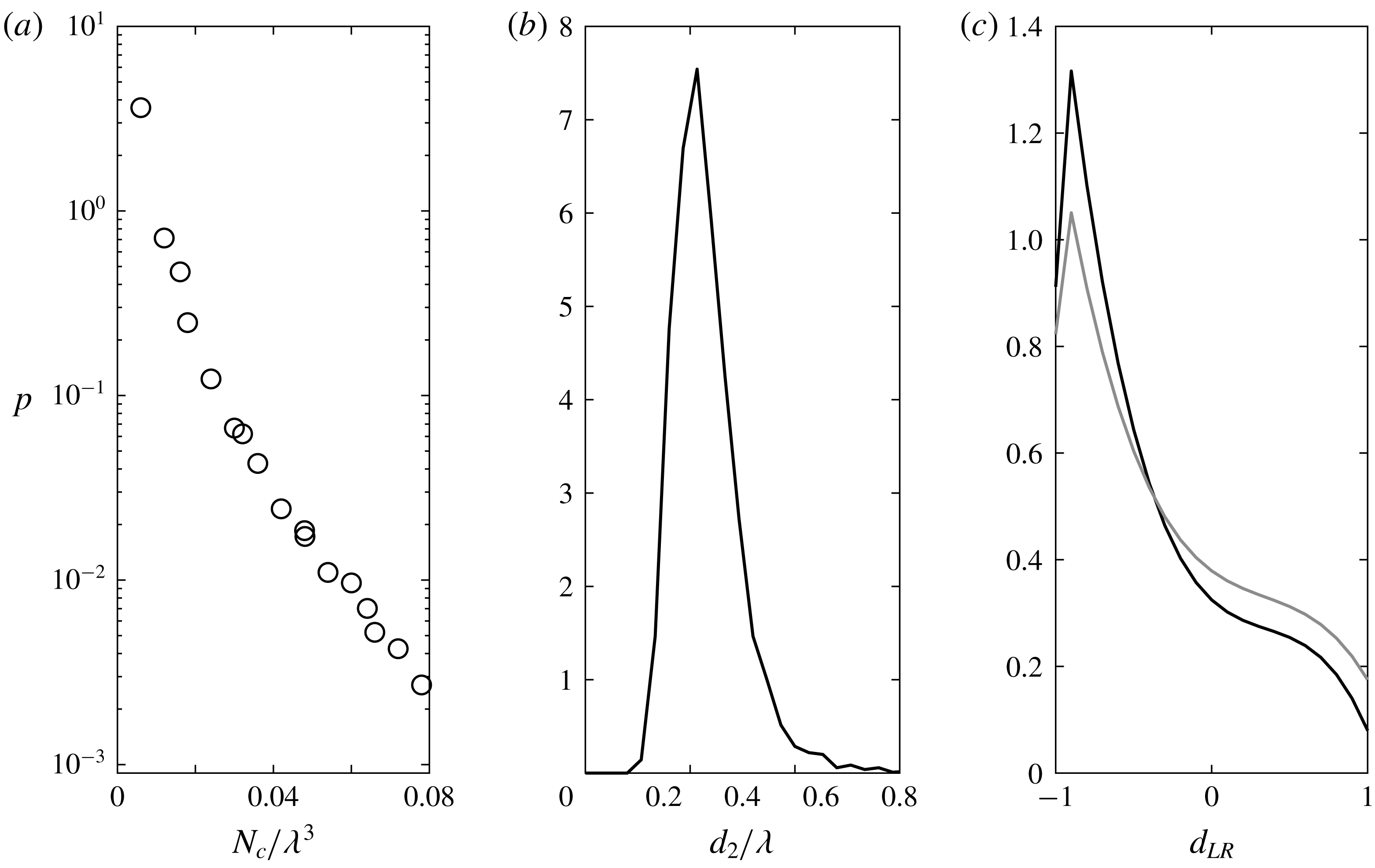
Probability distribution functions for various measures of the size and shape of regions fulfilling the
 $\ell =1$
criterion. Panel (a) is the probability density of the number of adjacent VGTs in a cluster,
 $N_{c}$
. Panel (b) gives the intermediate axis,
 $d_{2}$
for ellipsoids fitted to all the resolved clusters, defined as those consisting of more than eight VGTs. Panel (c) shows the shape of the resolved clusters applying the normalisation of Lund & Rogers (Reference Lund and Rogers1994) to the principal axes of the fitted ellipsoids,
 $\unicode[STIX]{x1D625}_{LR}$
in black. The shape of the flow structures within which these
 $\ell =1$
clusters are embedded is given by the grey line. This value is dimensionless, while those for
 $N_{c}^{1/3}$
and
 $d_{2}$
are non-dimensionalised by the Taylor scale,
 $\unicode[STIX]{x1D706}$
.

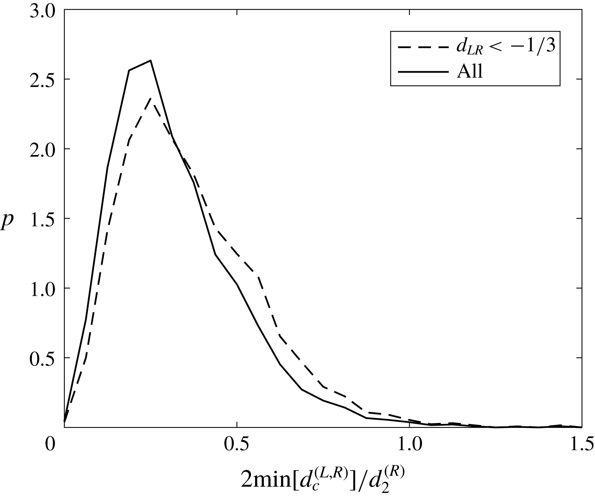
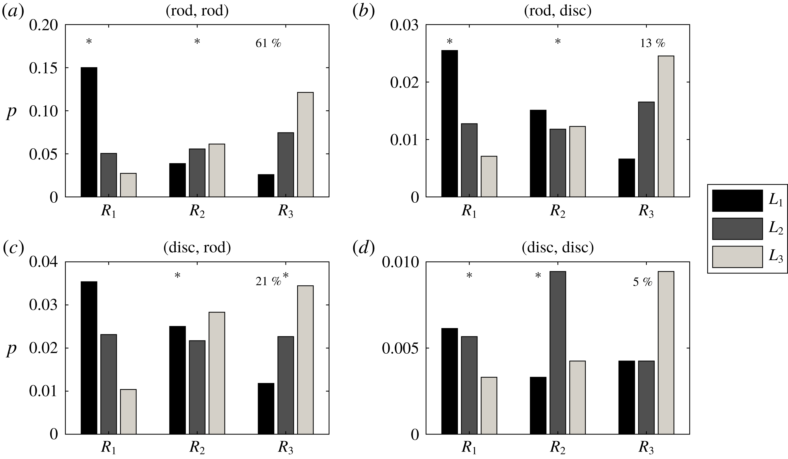
In a Euclidean frame, we extracted the tensors for which
 $\ell =1$
and then used a 26-connectivity (i.e. a legitimate neighbour to a point is any adjoining location on a cubic lattice) to define, groupings of adjacent tensors at the Lee bound. This was done by first forming a search list of all tensors with
 $\ell =1$
. Starting with the first on the list, any
 $\ell =1$
neighbours were found. If they existed, this was repeated until there were no new neighbours. These tensors were then grouped together and removed from the search list. The new tensor at the top of the list was then examined, and this continued until the search list was empty. The size of a cluster,
 $N_{c}$
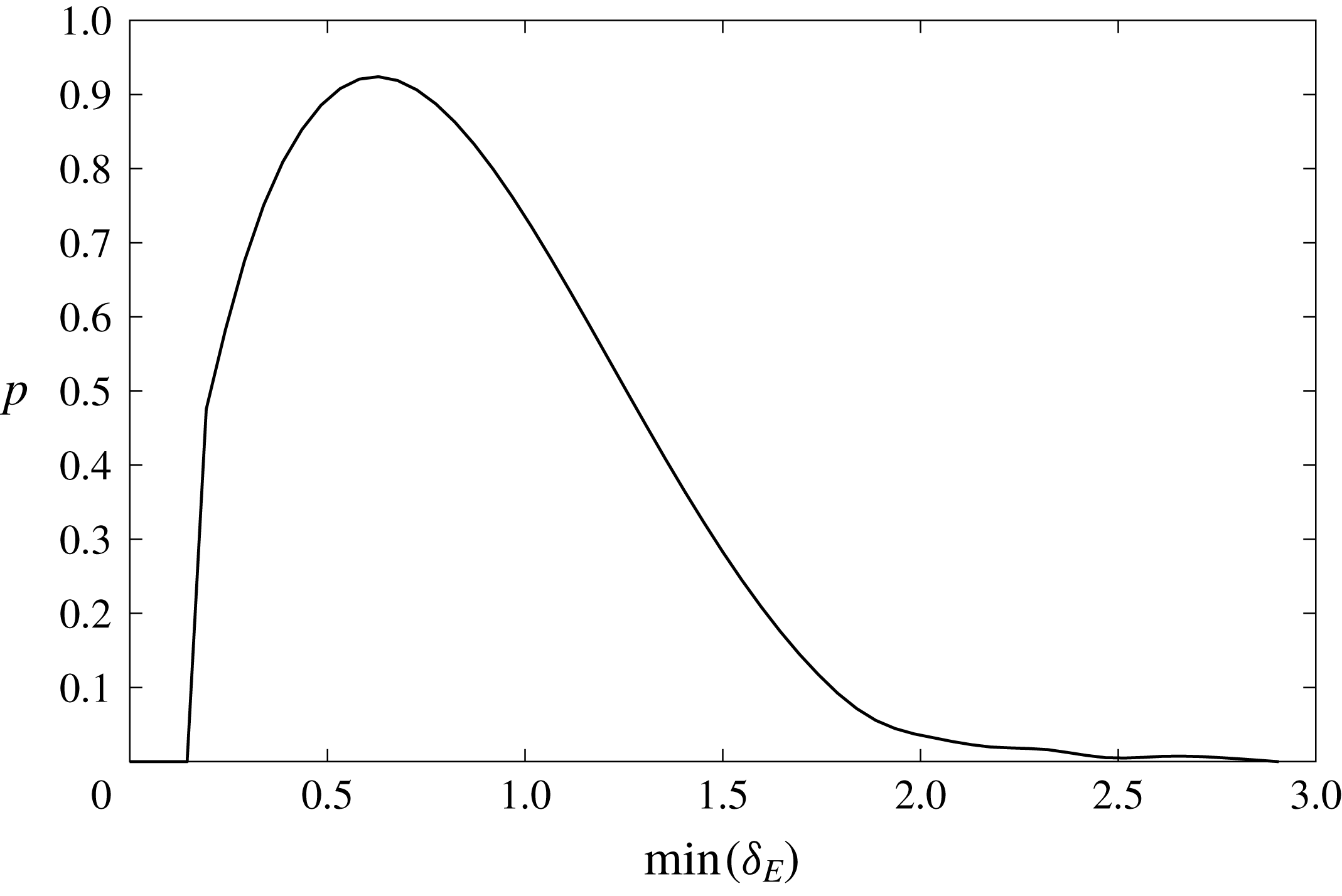
, in terms of the total number of adjoining tensors was then determined. Figure 9(a) shows the distribution function for the cluster sizes scaled by the cube of the Taylor scale. Defining the minimum resolution of the clustering as a group involving eight tensors (so that the cube root is two tensors), the number density of these resolved clusters was
 $0.85\unicode[STIX]{x1D706}$
. Looking more specifically at the minimum Euclidean distance,
 $\unicode[STIX]{x1D6FF}_{E}$
between centroids of these clusters, we obtain the results shown in figure 10 which has a median spacing of
 $0.80\unicode[STIX]{x1D706}$
, but with sufficient variance and positive skew that values of
 $\unicode[STIX]{x1D6FF}_{E}=2\unicode[STIX]{x1D706}$
are also possible. This presumably reflects, in part, an anisotropy in the shape of the flow structures to which the
 $\ell =1$
regions are associated. An ellipsoid was fitted to the groups of tensors exceeding the minimum resolution and the three principal axes for the ellipsoid,
 $d_{i}$
were determined. The mean subtracted values were then derived,
 $d_{i}^{\prime }=d_{i}-\langle d_{i}\rangle$
, and then the shape of the ellipsoid was determined by using the same normalisation that Lund & Rogers (Reference Lund and Rogers1994) introduced for examining the eigenvalues of the strain rate tensor
 $$\begin{eqnarray}\unicode[STIX]{x1D625}_{LR}=\frac{\displaystyle -3\sqrt{6}\prod \mathop{d}_{i}^{\prime }}{\displaystyle \left[\sum (\mathop{d}_{i}^{\prime })^{2}\right]^{3/2}}.\end{eqnarray}$$
The distribution for
 $\unicode[STIX]{x1D625}_{LR}$
is shown in figure 9(c) and it is clear that there is a tendency to form rod-like structures, i.e. a tendency towards the
 $\unicode[STIX]{x1D625}_{LR}=-1$
limit, with a median value of
 $\unicode[STIX]{x1D625}_{LR}=-0.55$
. The elongated nature of these
 $\ell =1$
structures helps explain the long positive tail to the distribution in figure 10. In contrast, the eigenvalues of the strain rate tensor preferentially form disc-like structures (Li & Meneveau Reference Li and Meneveau2007), as may be inferred from the existence of the Vieillefosse tail to the
 $Q_{A}-R_{A}$
diagram (Vieillefosse Reference Vieillefosse1984). Hence, it is potentially surprising that the grey line in figure 9(c) shows that the coherent structures within which the
 $\ell =1$
filaments are embedded also tend to have a rod-like shape, although this tendency is weaker than for the
 $\ell =1$
regions.
A probability density function of the minimum Euclidean distance between
 $\ell =1$
clusters, expressed as multiples of the Taylor scale.

The resolved clusters almost exclusively consisted of
 $\ell =1$
results for regions 1 and 2, with fewer than 1 % of these clusters having a contribution from regions 3 or 5. Consequently, occurrences of tensors at the Lee bound in regions 3 and 5 are a much less spatially extensive phenomenon. When they did occur in these resolved clusters, it was a single tensor within the group for 92 % of cases (of which in 63 % of cases it was a tensor from region 5 that contributed). This difference in spatial extent, combined with the relatively low frequency of Lagrangian trajectories involving
 $\ell =1$
tensors in regions 3 and 5 as demonstrated by table 3 means that these
 $\ell =1$
occurrences are transient, ‘one-off’ occurrences that arise close to the discriminant function,
 $\unicode[STIX]{x1D6E5}=0$
, below which
 $\Vert \unicode[STIX]{x03A9}_{B}\Vert =0$
(recall that the bound is dictated by
 $\unicode[STIX]{x03A9}_{A}$
for
 $Q<0$
).
In addition to the resolved clusters being overwhelmingly dominated by contributions from regions 1 and 2, it is also of note that the mix of contributions from these two regions was almost equally likely (tensors from region 1 made up 49 % of the tensors in a cluster, with a standard deviation of 7 %, a coefficient of skewness of 0.01 and of kurtosis of 3.12). This is in agreement with the results presented earlier that there is a typical behaviour for the flow at the Lee bound in regions 1 and 2, which makes attainment of this state equally likely despite the fact that on average, the flow is in region 2 for 2.4 times as many cases (figure 1).
The distribution for the length of the intermediate axis of the fitted ellipsoids is given in figure 9(b) and has a mode of
 $0.23\unicode[STIX]{x1D706}$
. As
 $d_{2}$
for the resolved clusters increased, the mean of 49 % occurrences from region 1 stayed the same meaning that this balance of contributions from region 1 and 2 is not a function of size. For example, when only considering cases for which
 $d_{2}>0.5\unicode[STIX]{x1D706}$
(the extreme upper tail as seen in figure 9
b), the mean was still 49 % with a standard deviation of 3 %.
5.2 The location and orientation of coherent regions where
$\ell =1$

A probability density function of the minimum Euclidean distance between the centroid of an
 $\ell =1$
resolved structure and the centroid of the larger coherent structure within which it is embedded. These distances are non-dimensionalised by the radius of the intermediate axis of the larger structure,
 $d_{2}^{(R)}$
. Results are shown for all
 $\ell =1$
structures and those which are rod-shaped based on
 $\unicode[STIX]{x1D625}_{LR}<-\frac{1}{3}$
.

As already stated, in those instances where extended regions are identified with
 $\ell =1$
, such occurrences are completely dominated by region 1 or 2. Hence, they are innately embedded within coherent flow structures as defined using the simple criterion of
 $Q_{A}>0$
(Hunt, Wray & Moin Reference Hunt, Wray and Moin1988; Dubief & Delcayre Reference Dubief and Delcayre2000). Figure 11 shows the minimum Euclidean distance between the centre of the ellipsoid fitted to the
 $\ell =1$
regions and that for the centroid of the surrounding coherent structures. This distribution has a mode at approximately one quarter of the radius of the intermediate axis of the larger flow structure. This is true for all cases as well as the most rod-like
 $\ell =1$
regions where
 $\unicode[STIX]{x1D625}_{LR}<-\frac{1}{3}$
. Thus, at this distance from the centre, non-local contributions to strain rate and, thus, dissipation are maximal relative to the local dissipation component.
The relative frequency of different  as a function of the shape of the
 $\ell =1$
resolved clusters and the coherent structures within which they are embedded. Rods and discs are defined in terms of
 $\unicode[STIX]{x1D625}_{LR}<-\frac{1}{3}$
and
 $\unicode[STIX]{x1D625}_{LR}>\frac{1}{3}$
, respectively. Hence, panel (b) indicates that a
 $\ell =1$
structure with a disc-like topology is embedded in a
 $Q_{A}>0$
(i.e. regions 1 or 2) structure with a rod-like shape to the ellipsoid fitted to these points. The asterisks in each panel highlight the cases where the median for
 exceeds 0.9397 (the median angle lies within
 $\pm 20^{\circ }$
of perfect alignment between the respective eigenvectors).

As noted in figure 9(c), the
 $\ell =1$
filaments typically occur within rod-like structures. Denoting the eigenvectors for the ellipsoid for the
 $\ell =1$
structures as
 $\boldsymbol{L}_{j}$
and for the embedded, extended regions that surround them as
 $\boldsymbol{R}_{i}$
, and with the eigenvectors corresponding to the principal, secondary, tertiary axes ordered from 1 to 3, the strength of the alignments between these eigenvectors was examined. Results are presented in figure 12 as a function of the joint topology of the
 $\ell =1$
structures, where the value stated first in the panel caption is for the larger-scale structure, and that stated second is for the
 $\ell =1$
structure, where rod and disc are defined by
 $\unicode[STIX]{x1D625}_{LR}<-\frac{1}{3}$
and
 $\unicode[STIX]{x1D625}_{LR}>\frac{1}{3}$
, respectively. The height of each bar shows the proportion all
 $\ell =1$
structures where a particular combination of
 $\boldsymbol{R}_{i}$
and
 $\boldsymbol{L}_{j}$
had the strongest alignment. These are normalised such that the sum over all bars and over all panels is 1.0. That is, the results shown are for
 , where the over-arrow denotes the angle between the underlying terms. Columns with an asterisk are those where the median for
 was great enough that there was at most
 $\pm 20^{\circ }$
departure from perfect alignment. Hence, when both ellipsoids are rod-like in shape as shown in panel (a), the most frequently arising dominant alignments are between
 $\boldsymbol{R}_{1}$
and
 $\boldsymbol{L}_{1}$
, followed by
 $\boldsymbol{R}_{3}$
and
 $\boldsymbol{L}_{3}$
. The asterisks also show that the strongest alignments are between
 $\boldsymbol{R}_{1}$
and
 $\boldsymbol{L}_{1}$
and
 $\boldsymbol{R}_{2}$
and
 $\boldsymbol{L}_{2}$
. In other words, if the coherent structure is rod-like in shape, the rod-like
 $\ell =1$
structure is aligned with it; both are being extended by the principal axis (most positive eigenvalue). This situation accounts for 61 % of the cases studied as indicated by the percentage in panel (a). The results in panel (b) are qualitatively similar, but have very different topological implications as the disc-like
 $\ell =1$
region is expanding along its first two axes, but the secondary axis is aligned with a compressing secondary axis for the larger structure. While it is still true in panel (c) that the
 , and
 alignments are most frequent, the typically strongest alignments are for
 , and
 , which is a more stable configuration than that in panel (b) as all the associated mean-subtracted eigenvalues have the same sign. This may explain why a rod-like
 $\ell =1$
filament within a larger disc (21 % of cases) is more frequent than a disc-like
 $\ell =1$
filament within a larger disc-like structure (13 % of cases). The results in panel (d) clearly contrast with the others. The most frequent strongest alignments associated with
 , and
 , and the strongest alignments on average occurring for
 , and
 . However, again, all these alignments are between mean-subtracted eigenvalues of the same sign indicating that this rare configuration (5 % of cases) is potentially more stable than that shown in panel (b).
6 The topological nature of the
$\ell =1$
tensors

We identify various types of flow structure by adopting the method of Horiuti (Reference Horiuti2001). The starting point for this approach is the vortex identification criterion of Jeong & Hussain (Reference Jeong and Hussain1995), which is pressure based but may be expressed in terms of the eigenvalues of
 $\unicode[STIX]{x1D643}=\unicode[STIX]{x1D64E}_{A}^{2}+\unicode[STIX]{x03A9}_{A}^{2}$
. Given a determination of the mutual alignments between the vorticity vector,
 $\unicode[STIX]{x1D74E}_{A}$
, and the eigenvectors of
 $\unicode[STIX]{x1D643}$
,
 $e_{i}^{(H)}$
, the most strongly aligned eigenvector is found and its eigenvalue denoted by
 $e_{z}^{(H)}$
. The flow topology is then classified based on the signs of the two remaining eigenvalues:
(i)
$e_{+}^{(H)}\geqslant e_{-}^{(H)}>0$
– a cylindrical sheet wrapped around a vortex tube (type CS);(ii)
$e_{+}^{(H)}\geqslant 0\geqslant e_{-}^{(H)}$
– a flat sheet where vorticity and strain are comparable (type FS);(iii)
$0>e_{+}^{(H)}\geqslant e_{-}^{(H)}$
– the core of a vortex tube (type VT).


The nature of the flow topology in different regions of the
 $Q_{A}-R_{A}$
diagram for
 $\ell =0$
cases (dark grey) and
 $\ell =1$
(light grey). Results are shown for that subset of cases where
 . The percentages quoted in each panel are the contribution of that region to the total number of
 $\ell =0$
cases, the contribution of that region to the
 $\ell =1$
cases (round brackets), and the overall percentage occupancies for that region, also given in figure 1 (square brackets). The labels for three topological states indicate a cylindrical sheet (CS), flat sheet (FS) and a vortex tube (VT).

Figure 13 shows the nature of the flow topology in each region of the
 $Q_{A}-R_{A}$
diagram for all cases where there was a strong alignment between
 $\unicode[STIX]{x1D74E}_{A}$
and
 $\unicode[STIX]{x1D748}_{z}^{(H)}$
 , i.e.
 $\pm 10^{\circ }$
. This equated to 23.7 % of the overall results. In each panel the percentage without brackets is the contribution to
 $\ell =0$
results in that region, with round brackets is the contribution to
 $\ell =1$
results in that region, while the value in square brackets is the percentage occupancy of the given region in general. Overall, the total number of
 $\ell =1$
cases with a strong alignment was 1.6 % of the value for the number of strongly aligned
 $\ell =0$
occurrences. This indicates a stronger tendency for the
 $\ell =1$
cases to exhibit such an alignment given the overall relative frequency of 0.66 % quoted at the start of § 4.1.
It is very clear that the results for regions 1 and 2 indicate the occurrence of vortex tubes, in agreement with the analysis based on
 $\unicode[STIX]{x1D625}_{LR}$
in the previous section. The region that exhibits the greatest difference topologically between the
 $\ell =0$
and
 $\ell =1$
states is region 5, which yields a flat sheet 78 % of the time and a vortex tube or a curved sheet approximately 11 % of the time in each case for
 $\ell =0$
. In contrast, for
 $\ell =1$
, the curved sheet arises 52 % of the time, and the flat sheet 48 % of the time, which looks much more similar to the
 $\ell =0$
results for region 6 (59 % : 41 % for curved sheets compared with flat sheets). Dissipation is known to arise preferentially in the curved sheets that wrap around vortex tubes (Kerr Reference Kerr1985; Jimenez et al.
Reference Jimenez, Wray, Saffman and Rogallo1993; Kawahara Reference Kawahara2005; Horiuti, Yanagihara & Tamaki Reference Horiuti, Yanagihara and Tamaki2016) and a high degree of normal straining is particularly prevalent along the Vieillefosse tail (Keylock Reference Keylock2018). Hence, the region 5
 $\ell =1$
occurrences have a topology that favours dissipation relative to the
 $\ell =0$
cases in this region.
7 Conclusion
A recently introduced approach to studying the dynamics of the velocity gradient tensor places a focus on the normal and non-normal components (Keylock Reference Keylock2018). As such, it is useful to employ a tight bound on the degree of non-normality (Lee Reference Lee1995) to examine those regions in the flow field where non-normality is as large as possible, meaning that the anisotropic parts of the pressure Hessian are driving the dynamics. This bound is attained in a trivial fashion where the eigenvalues of the VGT are real because there is no normal contribution to enstrophy, i.e.
 $\Vert \unicode[STIX]{x03A9}_{B}\Vert =0$
. Regions 3 and 5 lie close to the discriminant function separating real and complex-valued eigenvalues in the
 $Q_{A}-R_{A}$
diagram. Here, the bound is attained in a transitory fashion as seen from how rarely
 $\ell =1$
occurrences are in these regions (figure 1), the absence of any long duration occurrences in these regions (table 3) and the observation that when such occurrences do arise, they are typically singular realisations, that do not occur in substantive clusters (discussion in § 5.1).
In contrast, in the enstrophy-dominated regions of the
 $Q_{A}-R_{A}$
diagram, there is a clear structure to the
 $\ell =1$
occurrences irrespective of the sign of
 $R_{A}$
. In terms of turbulence production, the probability distribution of the sum of the interaction and non-normal production terms has a consistent shape that lies closer to that typically arising for region 1, explaining the more efficient generation of
 $\ell =1$
states in this region (figure 4). In addition, when
 $\ell =1$
the production term that is greatest in magnitude on average is the non-normal production (figure 3), the opposite of what is generally the case. An examination of the size and shape of the connected regions where
 $\ell =1$
in regions 1 and 2 indicates that they typically occur in rod-shaped structures, embedded within, and aligned with, rod-shaped coherent flow structures (figure 9
c). However, the centre of the
 $\ell =1$
filaments are typically
 $\frac{1}{4}$
of the intermediate axis of the larger structure from its centre (figure 11), and the typical spacing between these filaments is
 $0.8\unicode[STIX]{x1D706}$
(figure 10).
Because these filaments typically consist of an equal number of VGTs from regions 1 and 2, their
 $Q_{A}-R_{A}$
diagram in the enstrophy-dominated regions is symmetric, which is in contrast to what would appear to be the universality of the teardrop shape to the
 $Q_{A}-R_{A}$
diagram for the small-scale statistics of a number of developed or decaying turbulent flows (Laizet, Vassilicos & Cambon Reference Laizet, Vassilicos and Cambon2013; Gomes-Fernandes, Ganapathisubramani & Vassilicos Reference Gomes-Fernandes, Ganapathisubramani and Vassilicos2014; Laizet, Nedić & Vassilicos Reference Laizet, Nedić and Vassilicos2015; Zhou et al.
Reference Zhou, Nagata, Sakai, Ito and Hayase2016; Paul, Papadakis & Vassilicos Reference Paul, Papadakis and Vassilicos2017) at high Reynolds number. However, research that uses a modal decomposition such as proper orthogonal decomposition to define coherent structures from the leading modes has found that the
 $Q_{A}-R_{A}$
for the coherent part also has a high degree of symmetry in the enstrophy-dominated region (e.g. figure 6 of Buxton et al. (Reference Buxton, Breda and Chen2017)). Given that the majority of Lagrangian paths where
 $\ell =1$
in enstrophy-dominated regions either cross from regions 1 to 2 or vice versa or are initiated just after such a change (table 3), while they do not typically have their centroid in the centre of a coherent flow structure (figure 11), the
 $\ell =1$
regions are, in a sense, the centre of the coherent structure as they represent transitions in the signs of the local enstrophy production and strain production terms. Further work is needed to determine if there is a Reynolds number dependence to the frequency, spatial extent and location of the
 $\ell =1$
structures relative to the surrounding vortical motion. Such a study would complement recent work by Das & Girimaji (Reference Das and Girimaji2019) whose investigation into Reynolds number dependencies has suggested a limit of
 $Re_{\unicode[STIX]{x1D706}}\sim 6$
below which the teardrop shape of the
 $Q_{A}-R_{A}$
diagram does not arise for HIT.
The work by Goto & Vassilicos (Reference Goto and Vassilicos2009) discussed in the introduction stated that the dissipation coefficient in turbulence is a function of the stagnation point structure, which is in turn a function of the vortical behaviour given that these scale with the Taylor length,
 $\unicode[STIX]{x1D706}$
, and therefore help structure the location of stagnation points. The typical separation of the centroids of the resolved
 $\ell =1$
regions is
 $0.8\unicode[STIX]{x1D706}$
(figure 10) and these filaments within flow structures commonly occur at the interface of regions 1 and 2 where normal enstrophy production and normal strain production are changing sign. That the normal straining is tending to zero in these regions while the overall straining is approximately constant owing to the dominance of the non-local terms in these filaments (figure 8), means that the behaviour of the straining field and, thus, dissipation exhibits a subtle behaviour that is not evident using standard analyses. For the production terms, it is the non-normal production that is of greatest importance in such regions even though it is typically the smallest magnitude contribution to the production dynamics as shown in figure 3.
The dominance of non-normal terms in the
 $\ell =1$
filaments is important given the traditional focus on the invariants of the characteristic equation for the VGT. Because these are defined in terms of the eigenvalues they reflect the behaviour of the normal terms (Keylock Reference Keylock2018). Hence, correctly capturing the behaviour of these filaments provides a stringent test for models that step beyond the restricted Euler formulation and try to form compact and accurate models for the dynamics of the velocity gradient tensor (Martin et al.
Reference Martin, Dopazo and Valiño1998; Biferale et al.
Reference Biferale, Chevillard, Meneveau and Toschi2007; Wilczek & Meneveau Reference Wilczek and Meneveau2014; Johnson & Meneveau Reference Johnson and Meneveau2016).
Acknowledgement
Aspects of this research were supported by Royal Academy of Engineering/Leverhulme Trust Senior Research Fellowship LTSRF1516-12-89.