1 Introduction
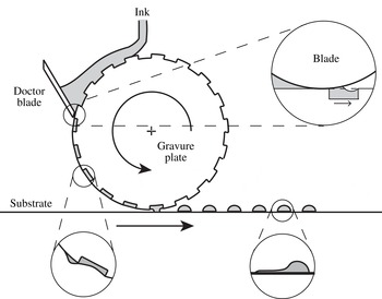
Intaglio printing is a transfer printing method and is suitable for low-cost, large area and high-throughput printing. A type of intaglio printing method is gravure printing, which has been used in a variety of industrial applications such as printing of photovoltaic modules, thin film transistors and polymer light emitting diodes (Søndergaard, Hösel & Krebs Reference Søndergaard, Hösel and Krebs2013). Figure 1 shows a basic schematic of gravure printing. A gravure roll with engraved cells translates beneath a stationary blade. Liquid placed upstream of the blade fills the cells as they enter the gap between the blade and substrate. The objective of the blade is to wipe the excess liquid from the unengraved parts of the gravure roll leaving liquid-filled cells. The pattern defined by those cells can then be printed onto another substrate by a transfer method.
Schematic of gravure printing.

Femtolitre intaglio (gravure) printing is one of the printing methods which includes transfer of ink to print electronics. A representative length scale of the method is three orders of magnitude smaller than the conventional gravure printing used for printing books, newspapers etc. In the conventional size printing, any defect smaller than
 $50~\unicode[STIX]{x03BC}\text{m}$
cannot be recognized by the human eye (Kumar Reference Kumar2015). In the printed electronics, on the other hand, micron-sized defects degrade the printed features at this scale. For instance, the organic field-effect transistor (OFET) is an example of printed electronics. It consists of several layers to be printed and the layer patterning should be precise, except for the dielectric layer. The precision of the printed source/drain electrodes determines the OFETs function (Kang, Lee & Cho Reference Kang, Lee and Cho2013). These electrodes are rectangular channels whose length and width affect the function, therefore any defect in the pattern affects the performance. Smaller channel length increases the operating speed of the transistor (Noh et al.
Reference Noh, Zhao, Caironi and Sirringhaus2007); however, as the patterns become smaller, defects become more important throughout the printing process.
Kitsomboonloha et al. (Reference Kitsomboonloha, Morris, Rong and Subramanian2012) describe the deposition of femtolitre drops by the gravure method. In their experiments, the substrate (gravure plate) translates beneath a stationary blade. In plan view, engraved cells are square with an edge length ranging from 1 to
 $10~\unicode[STIX]{x03BC}\text{m}$
; the cell depth is half the edge length.
Liquid placed on the substrate upstream of the blade fills the cells as they enter the gap between the blade and substrate. As each cell leaves the blade, some liquid is drawn from the cell (top magnified view in figure 1) and left behind as a tail on the substrate later in time (bottom left magnified view in figure 1) and that tail smears the printed feature (bottom right magnified view in figure 1). Over the range of capillary number (
 $Ca=\unicode[STIX]{x1D702}U/\unicode[STIX]{x1D6FE}$
, based on dynamic viscosity
 $\unicode[STIX]{x1D702}$
, substrate velocity
 $U$
and surface tension
 $\unicode[STIX]{x1D6FE}$
) studied by Kitsomboonloha et al. (Reference Kitsomboonloha, Morris, Rong and Subramanian2012), tails were always present; tail length is comparable with the cell length for
 $Ca=1$
and increases as
 $Ca$
is reduced. Maximum tail width (dimension normal to substrate velocity) is comparable with cell width. As shown by Kitsomboonloha et al. (Reference Kitsomboonloha, Morris, Rong and Subramanian2012, figure 13), tails are manifested as smearing of printed features. Similar behaviour is described by Nguyen, Shin & Lee (Reference Nguyen, Shin and Lee2014) and by Secor et al. (Reference Secor, Lim, Zhang, Frisbie, Francis and Hersam2014).
Kitsomboonloha et al. (Reference Kitsomboonloha, Morris, Rong and Subramanian2012) propose that tails form owing to lateral wicking along the apparent line between the blade and substrate (figure 1 shows a cross-section in the
 $x$
–
 $y$
plane; lateral wicking refers to wicking of liquid in the
 $z$
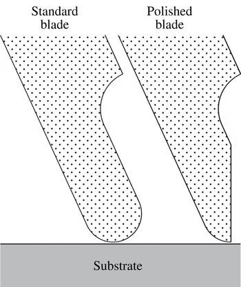
-direction which is the out of page direction considering figure 1). Because wicking requires liquid to wet the blade, tails could therefore be eliminated by making the blade non-wetting. By verifying experimentally that tails do not occur if the blade is non-wetting, Kitsomboonloha et al. (Reference Kitsomboonloha, Morris, Rong and Subramanian2012) demonstrate a connection between wettability and tail formation. Another way to reduce the tail formation is changing the blade geometry by polishing the tip of the blade. Figure 2 shows the plan view of the standard and polished blade tips. Polishing acts in plane, which can be thought of as a plane cut out of the page direction, and this increases the angle between the blade’s trailing edge face and substrate. As shown by Kitsomboonloha & Subramanian (Reference Kitsomboonloha and Subramanian2014), printed features become sharper when the blade tip is polished.
Blade tip for standard and polished cases.

It cannot be concluded that wicking causes tail formation, however. If the blade is assumed to be perpendicular to the substrate, lubrication theory holds throughout the entire liquid film if the cell is shallow and the contact angle
 $\unicode[STIX]{x1D703}$
on the blade is only slightly less than
 $90^{\circ }$
. By numerically solving the evolution equation describing the unsteady film, Ceyhan & Morris (Reference Ceyhan and Morris2014) show that tails form in plane flow (where wicking to the out of page direction cannot occur). They conclude that tail formation is a problem in plane Stokes flow. This conclusion leads us to the mechanism being analysed here.
We reduce the smear formation problem into two canonical problems: the first problem is the meniscus growth stage that we discuss in this paper; the second problem is tail formation extending back toward the blade which occurs at a later stage and is also of considerable hydrodynamic interest and is a problem we will discuss in another paper. In the limit as
 $Ca\rightarrow 0$
, a meniscus drawn from the cell is separated from the cell and that meniscus sitting between the blade and trailing edge of the cell is printed as a tail: the mechanism occurs between these two points, the cell is irrelevant. This limit shows that the problem can be connected to two other problems. The first one is the deposition of the tear film when we blink. Wong, Fatt & Radke (Reference Wong, Fatt and Radke1996) study the deposition and thinning of the human tear film. This film covers the exposed part of the eyeball by the rise of a meniscus of the upper lid during a blink and that meniscus is used to coat the tear film. The second problem is the liquid entrainment from the meniscus of a liquid wedge during coating (Gutenev, Pyatnitskii & Klimova Reference Gutenev, Pyatnitskii and Klimova2002; Reznik et al.
Reference Reznik, Salalha, Sorek, Avramov and Zussman2009). A film of tail shape is printed onto a horizontal substrate to be used in the deposition of micro–nano particle suspensions such as blood smears for histological analysis.
We outline the argument of this paper. As the leading edge of a liquid-filled cell emerges from beneath the blade, liquid rises on the blade to satisfy the Young condition (
 $\unicode[STIX]{x1D703}$
arbitrary). From our studies using lubrication theory, we know that the meniscus can be taken as being pinned to the leading edge of the cell: when the downstream nanometric coating film away from the cell has been included, that film almost touches the leading edge of the cell and we provide this effect by pinning the contact line there. As the cell moves away from the blade, its trailing edge eventually approaches the meniscus, isolating a certain volume of liquid from the cell. This isolated meniscus is then deformed by the drag exerted by the moving substrate. As far as the printing application is concerned, we believe the central problem to be that of minimizing the quantity of liquid drawn into the meniscus. The evolution of the isolated meniscus into a tail is, however, of considerable hydrodynamic interest, and will be treated in another paper.
In § 2, we formulate the initial boundary value problem (IBVP) and we explain the numerical method used to integrate the IBVP in § 3. In § 4, we give a geometric analysis of meniscus growth; this (hydrostatic) analysis describes the limit of vanishing capillary number
 $Ca$
based on substrate speed
 $U$
. To avoid detail, we initially take the blade to be perpendicular to the substrate and the contact angle over the blade to be at its static value. In reality, however, throughout the wiping process, the contact line over the blade first advances and then retreats; the static contact angle is in between the advancing contact angle
 $\unicode[STIX]{x1D703}_{A}$
and receding contact angle
 $\unicode[STIX]{x1D703}_{R}$
due to hysteresis:
 $\unicode[STIX]{x1D703}_{R}<\unicode[STIX]{x1D703}<\unicode[STIX]{x1D703}_{A}$
. If the hysteresis was taken into account during the meniscus growth stage, the hysteresis would decelerate the meniscus rise, and this would not violate the upper bound set by the current analysis in which we set the contact angle to its static value. In the tail formation stage, on the other hand, hysteresis would decelerate printing of the accumulated meniscus and this would increase the tail length. In this paper, we discuss the meniscus growth process; tail formation is not addressed and this is planned for a paper to follow. Here our point is to explain the physical mechanism of the meniscus growth process and show that there is an upper bound set by the hydrostatic limit. Evidently the hydrostatic theory would be of limited interest if viscous (normal) stresses exerted by the blade or hysteresis caused even more liquid to be removed from the cell. In § 5, numerical solutions of the free-boundary problem for the Stokes equations of motion are used to show that the hydrostatic theory closely describes the process of meniscus formation if
 $Ca<10^{-2}$
; moreover, as
 $Ca$
is increased, less liquid is removed from the cell. Because hydrostatics provides an upper bound to the volume removed, the problem of controlling tail formation now reduces to the conceptually simpler problem of reducing the size of the meniscus. In § 6, we use the hydrostatic theory to explain why Kitsomboonloha & Subramanian (Reference Kitsomboonloha and Subramanian2014) were able to minimize smearing by polishing the blade to reduce its tip radius.
2 Boundary value problem
Owing to small size of the engraved cell, the flow is not affected by inertial and gravitational forces. Defined by fluid density
 $\unicode[STIX]{x1D70C}$
, fluid dynamic viscosity
 $\unicode[STIX]{x1D702}$
, surface tension
 $\unicode[STIX]{x1D6FE}$
, substrate speed
 $U$
, characteristic cell size
 $L$
and gravitational acceleration
 $g$
; Reynolds number (
 $Re=\unicode[STIX]{x1D70C}UL/\unicode[STIX]{x1D702}<10^{-6}$
) and Bond number (
 $Bo=\unicode[STIX]{x1D70C}gL^{2}/\unicode[STIX]{x1D6FE}<10^{-8}$
), both are small compared with one. The flow is governed by the Stokes equations of motion.
Our objective here is to analyse smear formation without any complications. Because the radius of curvature
 $r$
of the blade tip is large compared with a representative length scale of the cell, such as its length
 $L$
, we initially model the blade tip as flat with its trailing edge face perpendicular to the substrate (considering the angle
 $\unicode[STIX]{x1D6FD}$
between the
 $x$
-axis and the blade face to be
 $\unicode[STIX]{x03C0}/2$
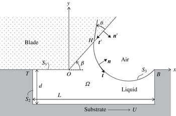
in figure 3). The cell is assumed to be full of liquid when it enters the gap between the blade and the substrate. This assumption is valid if there is no air entrainment into the cell. In the experiments, there is no evidence of air entrainment: see the tail formation photographs taken right after the wiping stage (figure 8 of Kitsomboonloha et al. (Reference Kitsomboonloha, Morris, Rong and Subramanian2012)).
Flow domain
 $\unicode[STIX]{x1D6FA}$
for the Stokes problem of smearing:
 $S_{1}$
, wiper blade;
 $S_{2}$
, cell boundary;
 $S_{3}$
, free surface. Coordinate axis is fixed on wiper blade which is stationary, cell translates with velocity
 $U\boldsymbol{i}$
.
 $T$
is the trailing edge,
 $B$
is the leading edge of the cell and the contact line meets the blade at
 $H$
. The aspect ratio of the cell is set to
 $L/d=2$
where
 $L$
is the length of the cell,
 $d$
is the depth of the cell.

Figure 3 shows the geometry of the model. As discussed in § 1, at the leading edge
 $B$
of the cell, the air–liquid interface
 $S_{3}$
is pinned; at the triple junction
 $H$
on the blade, the contact angle
 $\unicode[STIX]{x1D703}$
is prescribed. Right-handed axes
 $Oxyz$
are fixed in the blade, with origin
 $O$
as shown. On the air–liquid interface, the unit normal
 $\boldsymbol{n}$
is directed into the air; the unit tangent
 $\boldsymbol{t}=\boldsymbol{n}\times \boldsymbol{k}$
, with
 $\boldsymbol{k}$
denoting the unit vector along the
 $Oz$
axis. On the blade, the unit normal
 $\boldsymbol{n}^{\prime }$
is directed into the air; the unit tangent
 $\boldsymbol{t}^{\prime }=\boldsymbol{n}^{\prime }\times \boldsymbol{k}$
. Using as scales, cell length
 $L$
, substrate speed
 $U$
and dynamic viscosity
 $\unicode[STIX]{x1D702}$
of the liquid, we introduce dimensionless variables. We state the governing equations, then interpret them. The unknowns are the velocity vector
 $\boldsymbol{u}=u_{x}\boldsymbol{i}+u_{y}\,\boldsymbol{j}$
, stress tensor
 $\unicode[STIX]{x1D64F}$
and interface location
 $y=\unicode[STIX]{x1D701}(x,t)$
. Within the region
 $\unicode[STIX]{x1D6FA}$
occupied by liquid,
 $\boldsymbol{u}$
and
 $\unicode[STIX]{x1D64F}$
satisfy
 $$\begin{eqnarray}\displaystyle & \displaystyle \unicode[STIX]{x1D735}\boldsymbol{\cdot }\boldsymbol{u}=0, & \displaystyle\end{eqnarray}$$
 $$\begin{eqnarray}\displaystyle & \displaystyle \unicode[STIX]{x1D735}\boldsymbol{\cdot }\unicode[STIX]{x1D64F}=0, & \displaystyle\end{eqnarray}$$
 $$\begin{eqnarray}\displaystyle & \displaystyle \unicode[STIX]{x1D64F}=-p\unicode[STIX]{x1D644}+\unicode[STIX]{x1D735}\boldsymbol{u}+\unicode[STIX]{x1D735}\boldsymbol{u}^{\text{T}}, & \displaystyle\end{eqnarray}$$
 $$\begin{eqnarray}\displaystyle & \displaystyle \text{on }y=\unicode[STIX]{x1D701}(x,t),\quad \frac{\unicode[STIX]{x2202}\unicode[STIX]{x1D701}}{\unicode[STIX]{x2202}t}+u_{x}\frac{\unicode[STIX]{x2202}\unicode[STIX]{x1D701}}{\unicode[STIX]{x2202}x}=u_{y}, & \displaystyle\end{eqnarray}$$
 $$\begin{eqnarray}\displaystyle & \displaystyle Ca\unicode[STIX]{x1D64F}\boldsymbol{\cdot }\boldsymbol{n}=-\boldsymbol{n}(\unicode[STIX]{x1D735}\boldsymbol{\cdot }\boldsymbol{n}); & \displaystyle\end{eqnarray}$$
 $$\begin{eqnarray}\displaystyle & \displaystyle \text{at }H,\quad \boldsymbol{t}\boldsymbol{\cdot }\boldsymbol{t}^{\prime }=\cos \unicode[STIX]{x1D703}. & \displaystyle\end{eqnarray}$$
 $$\begin{eqnarray}\displaystyle & \displaystyle \text{On }S_{2},\quad \boldsymbol{u}=\boldsymbol{i}. & \displaystyle\end{eqnarray}$$
 $$\begin{eqnarray}\displaystyle & \displaystyle \text{On }S_{1},\quad \boldsymbol{u}\boldsymbol{\cdot }\boldsymbol{n}^{\prime }=0, & \displaystyle\end{eqnarray}$$
 $$\begin{eqnarray}\displaystyle & \displaystyle \boldsymbol{u}\boldsymbol{\cdot }\boldsymbol{t}^{\prime }=\left\{\begin{array}{@{}ll@{}}\ell \boldsymbol{t}^{\prime }\boldsymbol{\cdot }\unicode[STIX]{x1D64F}\boldsymbol{\cdot }\boldsymbol{n}^{\prime }\quad & \text{if }|\boldsymbol{r}-\boldsymbol{r}_{H}|<\ell \\ \ell \boldsymbol{t}^{\prime }\boldsymbol{\cdot }\unicode[STIX]{x1D64F}\boldsymbol{\cdot }\boldsymbol{n}^{\prime }\quad & \text{if }x_{T}<0\text{ and }x-x_{T}<\ell \\ \ell \boldsymbol{t}^{\prime }\boldsymbol{\cdot }\unicode[STIX]{x1D64F}\boldsymbol{\cdot }\boldsymbol{n}^{\prime }\quad & \text{if }x_{T}>0\text{ and }x<\ell \\ 0\quad & \text{otherwise}.\end{array}\right. & \displaystyle\end{eqnarray}$$
 $S_{1}$
, the Navier slip condition is applied within a distance of one slip length
 $\ell$
of the moving contact line
 $H$
; it is also applied within a distance
 $\ell$
of the intersection of the blade
 $S_{1}$
and substrate
 $S_{2}$
. This intersection occurs at
 $T$
if
 $x_{T}<0$
, but at
 $O$
if
 $x_{T}>0$
. By contrast, on the surface
 $S_{2}$
of the substrate, the no-slip condition is applied at all points, as stated by (2.1g
). Next, according to (2.1d
), the air–liquid interface
 $S_{3}$
is a material surface. We note that the only time derivative in the entire problem (2.1) appears in (2.1d
); a time derivative is, of course, not included in the Stokes equations of motion (2.1a
) and (2.1b
) because the time scale for vorticity diffusion is negligibly small in practice compared the time scale on which
 $S_{3}$
evolves. To obtain (2.1e
), we neglect the traction on the interface due to air and the Marangoni traction on the interface. Further, according to (2.1e
), on the interface
 $S_{3}$
, the shear stress vanishes and the normal stress balances the capillary pressure. Last, in (2.1f
), the contact angle
 $\unicode[STIX]{x1D703}$
is the static (Young) value; if the flow possesses a dynamic contact angle, that angle will appear as part of the solution of the free-boundary problem.
As initial state, we take the leading edge
 $B$
of the cell to be at
 $x/L=0.05$
; for the initial configuration of the interface, we use the hydrostatic solution obtained in § 4. Within slip regions, the Navier slip condition is imposed with slip length
 $\ell$
; all results are for
 $\ell /L=0.01$
, static contact angle
 $\unicode[STIX]{x1D703}=\unicode[STIX]{x03C0}/6$
and
 $L/d=2$
. For the element at the moving contact line, the length of the shortest edge was set equal to
 $0.1\ell$
.
Of course, viscous stress near the moving contact line distorts the interface and, if the calculation were inadequately resolved, the interface slope would vary abruptly near the blade. For results given here, the angle computed from the solution is always within
 $1^{\circ }$
of the imposed value of
 $30^{\circ }$
and with a slip length of 100 nm. This accuracy is consistent with the condition given by Sprittles & Shikmurzaev (Reference Sprittles and Shikmurzaev2012) for the minimum edge length of elements near a moving contact line.
3 Numerical method
We integrate the initial boundary value problem given in § 2 using a finite element method for the Stokes equations of motion (Peterson, Jimack & Kelmanson Reference Peterson, Jimack and Kelmanson1999; Johnson Reference Johnson2009; Ceyhan Reference Ceyhan2016) with isoparametric triangular elements.
The discretization of the variational problem (Johnson Reference Johnson2009, p. 232) is made using isoparametric triangular elements (Bathe Reference Bathe1996, figure 5.11) for the solution variables: the velocity components are interpolated using quadratic polynomials (
 $P2$
element), pressure is interpolated using a linear polynomial (
 $P1$
element). This choice of
 $P2$
–
 $P1$
element satisfies the Ladyzhenskaya–Babuška–Brezzi stability condition (Johnson Reference Johnson2009, p. 234).
The coordinates are interpolated using quadratic interpolation functions. Integrations are carried out exactly using a Gauss quadrature method using a seven-point Gauss integration rule for planes (Bathe Reference Bathe1996, §§ 5.5.4 and 5.5.5) and a three-point Gauss integration rule (Bathe Reference Bathe1996, § 5.5.3) for boundary integrals. We impose constraints on certain solution variables with the use of the Lagrange multiplier method. The unstructured mesh is generated using the methods explained by Persson (Reference Persson2004), Persson & Strang (Reference Persson and Strang2004).
Time integration is performed explicitly. At time
 $t$
, the linear Stokes problem is solved using the boundaries determined at the previous time
 $t-\unicode[STIX]{x0394}t$
; boundaries are then displaced in the normal direction to the interface using the velocity field from the same time
 $t-\unicode[STIX]{x0394}t$
. Because this method is explicit, we restrict the magnitude of
 $\unicode[STIX]{x0394}t$
using a Courant condition (Peterson et al.
Reference Peterson, Jimack and Kelmanson1999):
 $\unicode[STIX]{x0394}t<c\unicode[STIX]{x0394}x/u$
where
 $\unicode[STIX]{x0394}x$
is the minimum edge length in the mesh and
 $u$
is the maximum velocity. We take, for practical purposes,
 $c<1/4$
. This stability condition comes from the explicit integration of the kinematic boundary condition (2.1d
). Although the use of explicit integration of the kinematic boundary condition simplifies the implementation of the Stokes solver compared with the fully implicit higher-order integration rule, the restriction on the choice of time step slows the computation.
To maintain resolution, the quality of the mesh was checked regularly to refine the mesh; between refinements, the mesh was simply displaced from one time step to the next using the local fluid velocity. The mesh is dynamic so the number of elements varies throughout the integration. During mesh movement and remeshing, the mass of liquid must remain constant in the model problem for smear formation. In the corresponding computations, mass is conserved to within an error of
 $0.01\,\%$
. The method was also tested against problems in plane Stokes flow having explicit solutions: biharmonic problems such as flow through a slit, the problem of an overdamped capillary wave and the stick-slip problem (Richardson Reference Richardson1970) describing a free jet emerging from a slit in a thick wall. Galerkin formulation and discretization of the problem are described in appendix A.
4 Hydrostatics
4.1 Limit as
 $Ca\rightarrow 0$

In this section, we make an analysis in the limit as
 $Ca\rightarrow 0$
to show that the interface grows as a circular arc while emerging from beneath the wiper blade. Non-dimensionalized by the length scale
 $l_{s}=d$
, pressure scale
 $p_{s}=\unicode[STIX]{x1D6FE}/d$
and velocity scale
 $u_{s}=U$
where
 $d$
is the cell depth,
 $\unicode[STIX]{x1D6FE}$
is the surface tension and
 $U$
is the substrate speed; the dimensionless stress field is divergenceless:
 $$\begin{eqnarray}\displaystyle \unicode[STIX]{x1D735}\boldsymbol{\cdot }\unicode[STIX]{x1D64F}=\mathbf{0}. & & \displaystyle\end{eqnarray}$$
The non-dimensional Newtonian stress tensor is given by
 $$\begin{eqnarray}\displaystyle \unicode[STIX]{x1D64F}=-p\unicode[STIX]{x1D644}+Ca(\unicode[STIX]{x1D735}\boldsymbol{u}+\unicode[STIX]{x1D735}\boldsymbol{u}^{\text{T}}). & & \displaystyle\end{eqnarray}$$
In (4.2),
 $p$
is the dimensionless pressure field and
 $\boldsymbol{u}$
is the dimensionless velocity field. Continuity equation requires that velocity field is divergenceless:
 $$\begin{eqnarray}\displaystyle \unicode[STIX]{x1D735}\boldsymbol{\cdot }\boldsymbol{u}=0. & & \displaystyle\end{eqnarray}$$
Boundary conditions are given in § 2. The scales used in this section differ from § 2 therefore the normal component of the stress on the interface is different from (2.1e ). The interfacial boundary condition is now given by
 $$\begin{eqnarray}\displaystyle \boldsymbol{n}\boldsymbol{\cdot }(\unicode[STIX]{x1D64F}\boldsymbol{\cdot }\boldsymbol{n})=-\unicode[STIX]{x1D735}\boldsymbol{\cdot }\boldsymbol{n}. & & \displaystyle\end{eqnarray}$$
By defining the interface height as
 $\unicode[STIX]{x1D701}(x)$
measured from substrate level, we can write the outward unit normal on the interface by
 $$\begin{eqnarray}\displaystyle \boldsymbol{n}=\frac{\unicode[STIX]{x1D735}(y-\unicode[STIX]{x1D701}(x))}{|\unicode[STIX]{x1D735}(y-\unicode[STIX]{x1D701}(x))|}=\frac{\boldsymbol{e}_{y}-\boldsymbol{e}_{x}\unicode[STIX]{x1D701}_{x}}{(1+\unicode[STIX]{x1D701}_{x}^{2})^{1/2}}, & & \displaystyle\end{eqnarray}$$
and the curvature term is found to be
 $$\begin{eqnarray}\displaystyle \unicode[STIX]{x1D735}\boldsymbol{\cdot }\boldsymbol{n}=-\frac{\unicode[STIX]{x1D701}_{xx}}{(1+\unicode[STIX]{x1D701}_{x}^{2})^{3/2}}. & & \displaystyle\end{eqnarray}$$
By using (4.2), (4.3), (4.5) and (4.6), we can rewrite the interfacial boundary condition (4.4) as
 $$\begin{eqnarray}\displaystyle p+2Ca\left(\frac{\unicode[STIX]{x2202}u}{\unicode[STIX]{x2202}y}+\frac{\unicode[STIX]{x2202}v}{\unicode[STIX]{x2202}x}\right)\frac{\unicode[STIX]{x1D701}_{x}}{1+\unicode[STIX]{x1D701}_{x}^{2}}+2Ca\frac{\unicode[STIX]{x2202}u}{\unicode[STIX]{x2202}x}\frac{1-\unicode[STIX]{x1D701}_{x}^{2}}{1+\unicode[STIX]{x1D701}_{x}^{2}}=-\frac{\unicode[STIX]{x1D701}_{xx}}{(1+\unicode[STIX]{x1D701}_{x}^{2})^{3/2}}. & & \displaystyle\end{eqnarray}$$
The contact line is pinned at the leading edge of the cell and is free to move where the free surface meets the wiper blade. Although, as discussed by Cox (Reference Cox1986), when the contact line advances over the wiper blade the apparent contact angle is a flow property, the difference between the apparent contact angle and static (advancing) angle vanishes as the cube root of the
 $Ca$
based on the contact line velocity, so we assume the contact angle at the moving line over the wiper blade remains at its pre-defined static value given by
 $$\begin{eqnarray}\displaystyle \boldsymbol{t}\boldsymbol{\cdot }\boldsymbol{t}^{\prime }=\text{cos}(\unicode[STIX]{x1D703}). & & \displaystyle\end{eqnarray}$$
In the limit as
 $Ca\rightarrow 0$
,
 $\text{d}p/\text{d}x=0$
from (4.2). By taking the
 $x$
-derivative of (4.7) and integrating for the free surface profile, we find the free surface profile
 $\unicode[STIX]{x1D701}(x)$
, to a first approximation, to be a circular arc which is pinned at the leading edge of the cell and satisfying the contact angle condition (4.8) on the wiper blade. The shape of the interface is decoupled from the flow beneath itself; the meniscus grows as a circular arc. Now, we discuss the hydrostatic stage.
4.2 Geometric model
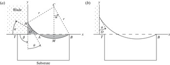
Figure 4 shows the geometry of the model; emerging and fully emerged cells are shown to emphasize that the analysis covers the evolution from the first state to the second. The coordinate system
 $xOy$
is orthogonal, with
 $x$
-axis along the surface of the substrate;
 $\unicode[STIX]{x1D6FD}$
denotes the angle between the blade and the
 $y$
-axis. Except in § 6,
 $\unicode[STIX]{x1D6FD}=\unicode[STIX]{x03C0}/2$
. We take the meniscus to be pinned at the leading edge
 $B$
of the cell.
Cell translating rightwards beneath a stationary blade occupying the second quadrant of the
 $xOy$
plane: (a) cell emerging; (b) cell fully emerged. See text for discussion.

In the limit as
 $Ca\rightarrow 0$
, viscous stress is negligibly small until the interface approaches the substrate. Until that occurs, liquid pressure is uniform and the meniscus is a circular arc
 $HMB$
. Point
 $A$
is the intersection of this arc with
 $OB$
;
 $CM$
is perpendicular to
 $OB$
. Arc
 $HMB$
has three degrees of freedom: its radius
 $r$
, and the coordinates of its centre
 $C$
. These variables are determined by the following conditions: because liquid that has risen above line
 $OB$
has been removed from the cell, the areas shaded in figure 4(a) are equal; the arc passes through
 $B$
; and it cuts the
 $y$
-axis at a given angle
 $\unicode[STIX]{x1D703}$
(Young angle). Here we should note that the equal area condition is valid assuming that no air is entrained during the wiping process.
The area of the shaded curvilinear triangle
 $OAH$
is given by
 $$\begin{eqnarray}\displaystyle |OAH|={\textstyle \frac{1}{4}}r^{2}\{4\cos \unicode[STIX]{x1D6FC}\cos \unicode[STIX]{x1D703}-\sin 2\unicode[STIX]{x1D6FC}-\sin 2\unicode[STIX]{x1D703}-\unicode[STIX]{x03C0}+2(\unicode[STIX]{x1D6FC}+\unicode[STIX]{x1D703})\}; & & \displaystyle\end{eqnarray}$$
as shown in figure 4(a),
 $\unicode[STIX]{x1D6FC}$
is the angle at which arc
 $AMB$
cuts the
 $x$
-axis at
 $A$
. The area of the shaded lens
 $AMB$
formed by chord
 $AB$
and the circular arc below
 $AB$
is given by
 $$\begin{eqnarray}\displaystyle |AMB|={\textstyle \frac{1}{2}}r^{2}(2\unicode[STIX]{x1D6FC}-\sin 2\unicode[STIX]{x1D6FC}). & & \displaystyle\end{eqnarray}$$
Equating areas, then simplifying, we obtain
 $$\begin{eqnarray}\displaystyle 4\cos \unicode[STIX]{x1D6FC}\cos \unicode[STIX]{x1D703}+\sin 2\unicode[STIX]{x1D6FC}=\sin 2\unicode[STIX]{x1D703}+\unicode[STIX]{x03C0}+2(\unicode[STIX]{x1D6FC}-\unicode[STIX]{x1D703}). & & \displaystyle\end{eqnarray}$$
Equation (4.11) holds until the trailing edge (point
 $T$
in figure 4
b) is at the interface.
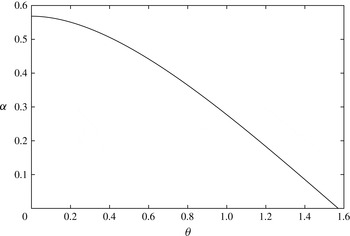
Figure 5 shows the change of
 $\unicode[STIX]{x1D6FC}$
as a function of
 $\unicode[STIX]{x1D703}$
. From (4.11), we see that
 $\unicode[STIX]{x1D6FC}$
is uniquely determined by the value of
 $\unicode[STIX]{x1D703}$
and so does not vary as the cell emerges. As
 $\unicode[STIX]{x1D703}$
is increased from zero to
 $\unicode[STIX]{x03C0}/2$
,
 $\unicode[STIX]{x1D6FC}$
decreases monotonically from 0.568 (about
 $33^{\circ }$
) to zero (see figure 5). In particular, equation (4.11) admits the solution
 $\unicode[STIX]{x1D6FC}=\unicode[STIX]{x1D703}=0.482$
(about
 $28^{\circ }$
).
The change of
 $\unicode[STIX]{x1D6FC}$
as a function of
 $\unicode[STIX]{x1D703}$
corresponding to (4.11).

From the geometry of figure 4, the arc radius
 $r$
is given in terms of
 $|OB|=b$
,
 $\unicode[STIX]{x1D6FC}$
and
 $\unicode[STIX]{x1D703}$
by
 $$\begin{eqnarray}\displaystyle b=r(\cos \unicode[STIX]{x1D703}+\sin \unicode[STIX]{x1D6FC}). & & \displaystyle\end{eqnarray}$$
Further, because
 $|OH|=h=r(\cos \unicode[STIX]{x1D6FC}-\sin \unicode[STIX]{x1D703})$
,
 $$\begin{eqnarray}\displaystyle h=b\frac{\cos \unicode[STIX]{x1D6FC}-\sin \unicode[STIX]{x1D703}}{\cos \unicode[STIX]{x1D703}+\sin \unicode[STIX]{x1D6FC}}. & & \displaystyle\end{eqnarray}$$
Because
 $\unicode[STIX]{x1D6FC}$
is fixed by (4.11), both the radius
 $r$
of the meniscus, and its height
 $h$
, are proportional to distance
 $b$
of the leading edge of the cell from the blade. In particular, the meniscus rises with constant velocity until the interface approaches the substrate. We note that, although viscosity is locally important near the advancing contact line, its effect there is merely to distort the interface locally, and so to produce the dynamic contact angle. That effect is irrelevant here; we are assuming that, in the limit as
 $Ca\rightarrow 0$
, the difference between the dynamic and static angles vanishes, as discussed by Hoffman (Reference Hoffman1975).
Viscous stress becomes essential to the process when the interface approaches the substrate. This can occur either if the trailing edge
 $T$
of the cell approaches the interface (points
 $A$
and
 $T$
coincide), or at the bottom of the cell (point
 $M$
approaches the cell bottom). In the first case, the hydrostatic stage ends when
 $|AB|$
is equal to the cell length
 $L$
. Because, from the geometry of figure 4(a),
 $|AB|=2r\sin \unicode[STIX]{x1D6FC}$
, the radius
 $r_{1}$
at the end of hydrostatic stage is given by
 $r_{1}=L/(2\sin \unicode[STIX]{x1D6FC}).$
In the second case, the hydrostatic stage ends when the distance of point
 $M$
to
 $OB$
is equal to the cell depth
 $d$
:
 $r-r\cos \unicode[STIX]{x1D6FC}=d$
. The corresponding value
 $r_{2}$
of the radius is
 $r_{2}=d/(1-\cos \unicode[STIX]{x1D6FC}).$
The cell aspect ratio
 $L/d$
determines which case is relevant. As the cell emerges,
 $r$
increases from zero and the hydrostatic stage ends when
 $r$
is equal to the smaller of
 $r_{1}$
and
 $r_{2}$
. Comparing the expressions for
 $r_{1}$
and
 $r_{2}$
, we find that
 $r_{1}<r_{2}$
if
 $$\begin{eqnarray}\displaystyle L/d<2\cot \left({\textstyle \frac{1}{2}}\unicode[STIX]{x1D6FC}\right). & & \displaystyle\end{eqnarray}$$
For perfect wetting (
 $\unicode[STIX]{x1D703}=0$
), equation (4.14) corresponds to
 $L/d<6.84$
. For marginal wetting (
 $\unicode[STIX]{x1D703}\rightarrow \unicode[STIX]{x03C0}/2$
), and
 $\unicode[STIX]{x1D6FC}\rightarrow 0$
: for this system, the hydrostatic stage ends when the trailing edge of the cell approaches the interface, even for a very long shallow cell. In the Kitsomboonloha et al. (Reference Kitsomboonloha, Morris, Rong and Subramanian2012) experiments, the cells are square in planform, with
 $L/d=2$
. Because this is within the range defined by (4.14), we now consider only the first case.
As a result of the trailing edge approaching the interface, liquid between
 $O$
and
 $A$
is isolated from the cell. We conclude that the amount of liquid removed from the cell is determined by hydrostatics, whereas viscosity will be important in determining how that fixed amount of liquid is smeared over the substrate. The mechanism producing tails operates solely between points
 $O$
and
 $A$
; the cell plays no further part.
The area
 $A_{\ast }$
removed from the cell of length
 $L$
is given by (4.10), with
 $r=r_{1}$
:
 $$\begin{eqnarray}\displaystyle A_{\ast }=L^{2}\frac{2\unicode[STIX]{x1D6FC}-\sin 2\unicode[STIX]{x1D6FC}}{8\sin ^{2}\unicode[STIX]{x1D6FC}}. & & \displaystyle\end{eqnarray}$$
As
 $\unicode[STIX]{x1D703}$
is increased from 0 to
 $\unicode[STIX]{x03C0}/2$
,
 $A_{\ast }/L^{2}$
decreases from
 $0.099$
to zero: for
 $\unicode[STIX]{x1D703}=\unicode[STIX]{x03C0}/2$
, there is no meniscus, and no liquid is lost from the cell. Further, because the cell area is
 $Ld$
, the ratio
 $A_{\ast }/(Ld)$
increases linearly with cell aspect ratio
 $L/d$
.
5 Viscous effects
Using numerical solutions of the free-boundary problem for the Stokes equations of motion, we demonstrate that the hydrostatic analysis provides an upper bound for the amount of liquid removed from the cell. We set the angle
 $\unicode[STIX]{x1D6FD}$
between the blade and substrate (figure 3) to
 $\unicode[STIX]{x03C0}/2$
for the following computations.
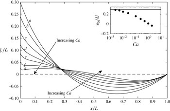
Interface shape at the instant
 $t=0.95$
the trailing edge of the cell leaves the blade;
 $L/d=2$
,
 $\unicode[STIX]{x1D703}=\unicode[STIX]{x03C0}/6$
. Curve (a) hydrostatic; curves (b–g), computed for
 $Ca=0.025,0.1,0.25,0.5$
, 1 and 2. Inset, ratio
 $v_{0}/U$
of contact line velocity to substrate velocity; solid line shows the static upper bound.

Figure 6 shows the interface height
 $\unicode[STIX]{x1D701}/L$
at the instant (
 $t=0.95$
) the trailing edge of the cell leaves the blade, corresponding to point
 $T$
in figure 4 coinciding with point
 $O$
. For
 $Ca=1$
(curve (f)) and
 $Ca=2$
(curve (g)), the interface slope is small (
 ${\sim}0.1$
) everywhere, except very near the blade where the contact angle condition requires the slope to be of the order of unity. As
 $Ca$
is decreased from curve (g) to curve (b) (
 $Ca=0.025$
), the interface approaches the static shape shown by curve (a). For clarity, curves for
 $Ca=0.01$
, 0.005 and 0.0025 are omitted from the figure; they are almost identical with curve (a).
The inset shows the contact line velocity
 $v_{0}$
along the blade at
 $x=0$
. According to the hydrostatic solution (4.13), the contact line rises with uniform speed until the trailing edge of the cell touches the interface; for
 $\unicode[STIX]{x1D703}=\unicode[STIX]{x03C0}/6$
,
 $v_{0}/U=0.298$
. The numerical solutions show that
 $v_{0}$
decreases markedly as
 $Ca$
is increased. To explain that effect, we show streamlines in the next figure.
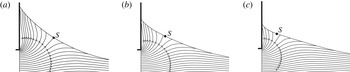
Figure 7 shows, in particular, the behaviour of the streamline that divides liquid rising along the blade from that moving rightwards with the substrate. In all three cases, the contact line is rising over the blade but, as the viscous pressure increases relative to capillary pressure (increasing
 $Ca$
), an increasing fraction of the liquid is pulled to the right. As a result, the dividing streamline moves leftwards along the interface; this is consistent with the flattening of the interface seen in figure 6.
Streamlines corresponding to curves (b–d) in figure 6. Region
 $0<x/L<0.5$
,
 $-0.125<y/L<0.25$
and (a),
 $Ca=0.025$
; (b), 0.10 and (c) 0.25;
 $S$
is the separatrix.

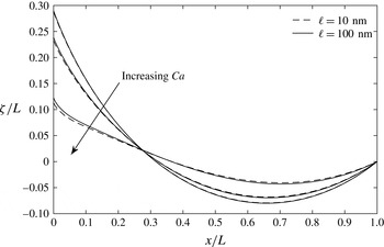
Effect of slip length corresponding to figure 6 for
 $Ca=0.0025$
, 0.025 and 0.25.

The choice of relatively high slip length of 100 nm instead of realistic values of 1–10 nm (Eggers Reference Eggers2005) has two bases. The first is the observation of the effect of slip length on the behaviour of the free surface profile. We show the effect of slip length in figure 8: decreasing the slip length to 10 nm does not affect the free surface movement for
 $Ca<0.1$
compared with the slip length of 100 nm, and the computed angles at the contact line are within an error of
 $1^{\circ }$
. When the
 $Ca$
is
 $O(1)$
, however, the computed angle is within an error of
 $3^{\circ }$
and this effect is visible in the direction of increasing
 $Ca$
in figure 8. Beside, during meniscus growth stage, the upper bound set by the hydrostatic theory is not violated by the slip length’s being in the range of 10–100 nm. The second basis is on the account of computational element size. To be able to resolve the region within an error of
 $1^{\circ }$
requires the smallest element size to be 0.1
 $\ell$
for capillary number
 $O(1)$
(Sprittles & Shikmurzaev Reference Sprittles and Shikmurzaev2012). With the current version of our numerical method, due to explicit time integration and the relatively complex computational domain, we are not able to go down to the realistic slip length range for the whole range of
 $Ca$
studied. To be consistent in all the computations, we set the slip length to 100 nm.
Interface shape at the instant
 $t=1.35$
the trailing edge of the cell is at
 $x/L=0.4$
. For
 $\unicode[STIX]{x1D703}$
and
 $L/d$
, see caption to figure 6. Curve (a), hydrostatic; curves (b–e), computed for
 $Ca=0.0025,0.005,0.01$
and
 $0.025$
. Inset, ratio
 $v_{0}/U$
of contact line velocity to substrate velocity.

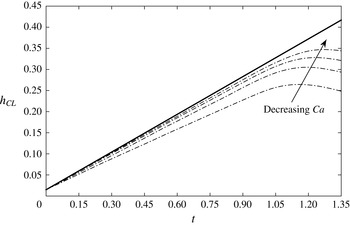
The history of contact line position
 $h_{CL}$
over the blade: ——, static prediction; — ⋅ —, computed for
 $Ca=0.0025,0.005,0.01$
and
 $0.025$
.

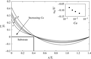
Figure 9 shows the interface height at a later time (
 $t=1.35$
). The trailing edge
 $T$
of the cell has now advanced to
 $x/L=0.4$
; this value of
 $x/L$
is slightly less than that (
 $0.460$
) at which the hydrostatic analysis predicts that
 $T$
reaches the interface. Curve (e) for
 $Ca=0.025$
shows the later stage of the solution given as curve (b) in figure 6: there, viscosity has only a modest effect on interface shape. By contrast, the inflection on curve (e) shows that viscosity now has a significant effect: for the larger values of
 $Ca$
, the meniscus is beginning to be printed.
The pronounced effect of viscosity is also apparent in the inset showing the ratio
 $v_{0}/U$
: even for the smallest value of
 $Ca=0.0025$
, the contact line is retreating (
 $v_{0}/U\simeq -0.08$
), whereas in the hydrostatic solution, the contact line advances with uniform speed (
 $v_{0}/U=0.298$
) until the trailing edge of the cell touches the interface.
Figure 10 shows the evolution of contact line position over the blade. The contact line velocity changes sign before the interface touches the edge of the cell; the moment when the printing starts is the point of maximum at each curve for the computed solutions in figure 10: as
 $Ca$
is decreased, the printing of the meniscus starts later; and the family of curves shows that the solution approaches the static prediction (solid line in figure 10).
We note that we do not observe a transition to Landau–Levich–Derjaguin film for the receding contact line: no thin film is deposited on the blade
 $x=0$
. Two explanations offer themselves. First, the geometry differs from that in dip coating. Viscous stress here plays a double role; shear stress near the contact line promotes film deposition but substrate drag opposes it. Second, even if that effect were absent, as in dip coating or bubble flow in a tube, no film is deposited if the capillary number
 $Ca_{0}$
, based on contact line velocity
 $v_{0}$
, is less than a critical value:
 $Ca^{\prime }$
depends on static contact angle
 $\unicode[STIX]{x1D703}$
and, weakly, on slip length
 $\ell$
and on the radius
 $r$
of curvature of the outer meniscus (Quéré Reference Quéré1991, equation 5; Eggers Reference Eggers2005, equation 41). Because
 $Ca^{\prime }$
is an increasing function of
 $\ell /r$
, the relatively large value of
 $\ell /r\sim 10^{-2}$
used here would inhibit coating.
The preceding figures show that the area under the meniscus is a decreasing function of
 $Ca$
. It remains to show that, with decreasing
 $Ca$
, liquid is increasingly trapped as the trailing edge of the cell approaches the interface.
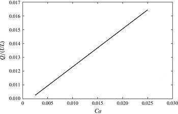
From figure 11, we see that, for the configuration shown in figure 9, the flow rate
 $Q=\int _{0}^{\unicode[STIX]{x1D701}}v_{x}\,\text{d}y$
through the restriction between the interface and trailing edge of the cell is
 ${\sim}1\,\%$
of the characteristic flow rate
 $UL$
within the cell itself. The ratio
 $Q/(UL)$
decreases linearly with a slope of 0.27 with decreasing
 $Ca$
. We conclude that hydrostatics provides an upper bound to the volume left behind on the substrate. The problem of minimizing smearing simplifies to one of reducing that upper bound.
Flow rate at the trailing edge of the cell; configuration as in figure 9.

6 Blade geometry
The smears shown in Kitsomboonloha et al. (Reference Kitsomboonloha, Morris, Rong and Subramanian2012, figure 7) were observed in experiments in which the cell length
 $L=7.5~\unicode[STIX]{x03BC}\text{m}$
, and the radius of the blade tip,
 $75~\unicode[STIX]{x03BC}$
m. Kitsomboonloha & Subramanian (Reference Kitsomboonloha and Subramanian2014, figure 8) show that printed features become sharper when the blade is polished to reduce the tip radius to 3
 $\unicode[STIX]{x03BC}$
m. To illustrate the hydrostatic theory, we use it to suggest why polishing is effective.
In the first case, the tip radius is
 $10L$
, and a careful sketch shows that the curved surface of the blade can be modelled, at the scale of the cell, by a flat blade making an acute angle
 $\unicode[STIX]{x1D6FD}$
with the
 $x$
-axis. (Though in figure 1(b) of Kitsomboonloha et al. (Reference Kitsomboonloha, Morris, Rong and Subramanian2012), the blade as a whole is shown as making an obtuse angle with the
 $x$
-axis, we are concerned here with the local angle where the cell leaves the blade; that angle is acute.)
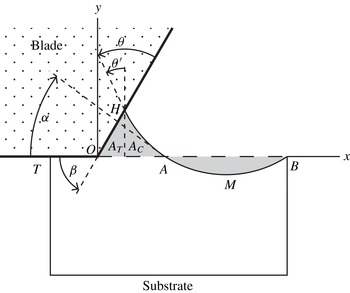
Geometry of tilted blade.

Figure 12 shows the geometry of the tilted blade. The angle made by the interface with the vertical at the contact line
 $H$
is now
 $\unicode[STIX]{x1D703}^{\prime }=\unicode[STIX]{x1D703}+\unicode[STIX]{x1D6FD}-\unicode[STIX]{x03C0}/2$
. The effect of tilting the blade is to create additional area beneath it. To illustrate this effect, we consider the case
 $\unicode[STIX]{x1D703}^{\prime }\geqslant 0$
in which the area
 $A$
of the meniscus can be calculated using results already given: to obtain the area
 $A_{C}$
of the curvilinear triangle formed by the interface,
 $x$
-axis, and abscissa passing through
 $H$
, we need only replace
 $\unicode[STIX]{x1D703}$
in (4.9) by
 $\unicode[STIX]{x1D703}^{\prime }$
. The other contribution is the area
 $A_{T}$
of the right triangle formed by that same abscissa, the blade, and
 $x$
-axis:
 $A_{T}=(r^{2}/2)(\cos \unicode[STIX]{x1D6FC}-\sin \unicode[STIX]{x1D703}^{\prime })^{2}\cot \unicode[STIX]{x1D6FD}.$
As
 $\unicode[STIX]{x1D6FD}$
is reduced,
 $A_{T}$
increases without bound. As far as the cell is concerned, tilting a flat blade creates a large volume sink.
Equating the total area
 $A=A_{C}+A_{T}$
to the area
 $|AMB|$
removed from the cell, then simplifying, we find that
 $\unicode[STIX]{x1D6FC}$
,
 $\unicode[STIX]{x1D6FD}$
and
 $\unicode[STIX]{x1D712}=\unicode[STIX]{x1D6FD}+\unicode[STIX]{x1D703}$
satisfy the relation
 $$\begin{eqnarray}\displaystyle 4\cos \unicode[STIX]{x1D6FC}\sin \unicode[STIX]{x1D712}+\sin 2\unicode[STIX]{x1D712}+\sin 2\unicode[STIX]{x1D6FC}+2(\cos \unicode[STIX]{x1D6FC}+\cos \unicode[STIX]{x1D712})^{2}\cot \unicode[STIX]{x1D6FD}=2(\unicode[STIX]{x03C0}+\unicode[STIX]{x1D6FC}-\unicode[STIX]{x1D712}). & & \displaystyle\end{eqnarray}$$
Because it is assumed in deriving (6.1) that
 $\unicode[STIX]{x1D703}^{\prime }\geqslant 0$
, the result holds for
 $\unicode[STIX]{x1D712}\geqslant \unicode[STIX]{x03C0}/2$
.
For
 $\unicode[STIX]{x1D703}=\unicode[STIX]{x03C0}/2$
, the condition
 $\unicode[STIX]{x1D712}\geqslant \unicode[STIX]{x03C0}/2$
is satisfied even for
 $\unicode[STIX]{x1D6FD}\ll 1$
. To obtain the solution of (6.1) in that case, we note that arc
 $AH$
in figure 12 then approximates to chord
 $AH$
. From the geometry of the triangle formed by the blade, chord
 $AH$
and the
 $x$
-axis,
 $\unicode[STIX]{x1D6FD}+\unicode[STIX]{x1D703}+\unicode[STIX]{x1D6FC}=\unicode[STIX]{x03C0}$
, whence
 $\unicode[STIX]{x1D6FC}\rightarrow \unicode[STIX]{x03C0}-\unicode[STIX]{x1D703}$
as
 $\unicode[STIX]{x1D6FD}\rightarrow 0$
. To obtain the next term in this approximation, we substitute the series
 $$\begin{eqnarray}\displaystyle \unicode[STIX]{x1D6FC}\sim \unicode[STIX]{x03C0}/2+c\unicode[STIX]{x1D6FD}^{1/2}, & & \displaystyle\end{eqnarray}$$
into (6.1), and find that
 $c=\sqrt{\unicode[STIX]{x03C0}}.$
Together, equation (4.15) and (6.1) determine the area
 $A_{\ast }$
that has been removed from the cell when its trailing edge reaches the interface.


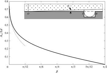
Figure 13 shows
 $A_{\ast }/(Ld)$
as a function of blade angle
 $\unicode[STIX]{x1D6FD}$
for contact angle
 $\unicode[STIX]{x1D703}=\unicode[STIX]{x03C0}/2$
. According to the results in § 6, for this value of
 $\unicode[STIX]{x1D703}$
, and blade angle
 $\unicode[STIX]{x1D6FD}=\unicode[STIX]{x03C0}/2$
, a negligibly small amount of liquid is removed:
 $A_{\ast }\rightarrow 0$
at the right end of the figure. At the other extreme,
 $\unicode[STIX]{x1D6FD}\rightarrow 0$
; in this case,
 $\unicode[STIX]{x1D6FC}\rightarrow \unicode[STIX]{x03C0}/2$
. The inset shows the corresponding meniscus: it is a semi-circle spanning the cell and having a little finger that reaches up to touch the blade, thereby completing the right triangle whose area is the quantity
 $A_{T}$
described above equation (6.1). It remains to verify that this extreme situation is not an artefact of assuming a flat blade.
Meniscus of a marginally wetting liquid beneath a parabolic blade.

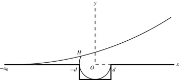
Figure 14 shows the corresponding situation for the parabolic blade
 $y=(x+x_{0})^{2}/(2\unicode[STIX]{x1D70C})$
, and cell aspect ratio
 $L/d=2$
. The coordinate origin
 $O$
is at the centre of the top of the cell; the ends of the cell are at
 $x=\pm d$
. The sketch is drawn to scale for
 $\unicode[STIX]{x1D700}=L/\unicode[STIX]{x1D70C}=0.1$
; it suggests that the following assumptions hold in the limit as
 $\unicode[STIX]{x1D700}\rightarrow 0$
: (i) the contact line is at
 $x=-L/2$
; (ii) when the trailing edge reaches the meniscus, as shown in the figure, the cell has emerged a distance
 $x_{0}\gg L$
; and (iii) the slope of the parabola at the contact line
 $H$
is vanishingly small. We assume, then verify, these properties. First, by assumption (i), the area of the meniscus is given by
 $A_{2}=\int _{-x_{0}}^{-L/2}y\,\text{d}x$
. Equating that area to the area
 $A_{1}=(L^{2}(1-\unicode[STIX]{x03C0}/4))/2$
removed from the cell, then using (ii) to neglect a small term of the order of
 $L/x_{0}$
, we find that in the limit as
 $\unicode[STIX]{x1D700}\rightarrow 0$
,
 $$\begin{eqnarray}\displaystyle x_{0}/L\sim 0.863/\unicode[STIX]{x1D700}^{1/3}; & & \displaystyle\end{eqnarray}$$
this justifies assumption (ii). Next, the contact line
 $H$
is located at the intersection of the parabola
 $y=(x+x_{0})^{2}/(2\unicode[STIX]{x1D70C})$
with the circular arc
 $x^{2}+y^{2}=L^{2}/4$
. Eliminating
 $y$
between these equations, then using (ii) to neglect terms of the order of
 $L/x_{0}$
, we find that point
 $H$
is located at
 $$\begin{eqnarray}\displaystyle x_{c}\sim -(L/2)(1-0.373\unicode[STIX]{x1D700}^{4/3}); & & \displaystyle\end{eqnarray}$$
this justifies assumption (i). Lastly, because
 $x_{0}\gg |x_{c}|$
, the slope of the parabola at
 $H$
is given by
 $x_{0}/\unicode[STIX]{x1D70C}\sim 0.863\unicode[STIX]{x1D700}^{2/3}$
. Because the slope of the parabola is vanishingly small, whilst that of the circular arc is large, the contact angle
 $\unicode[STIX]{x1D703}$
approaches
 $\unicode[STIX]{x03C0}/2$
from below:
 $$\begin{eqnarray}\displaystyle (\unicode[STIX]{x03C0}/2)-\unicode[STIX]{x1D703}\sim 0.863\unicode[STIX]{x1D700}^{1/3}. & & \displaystyle\end{eqnarray}$$
Maximum volume is withdrawn from the cell if the circular arc meniscus passes through the leading and the trailing vertices of the cell, and also touches the cell bottom; this occurs if the contact angle
 $\unicode[STIX]{x1D703}$
, cell length
 $L$
and blade radius of curvature
 $\unicode[STIX]{x1D70C}$
satisfy (6.5). We conclude that if the tip radius of the blade is large compared with the cell length, most of cell volume is drawn into the meniscus even for a marginally wetting system.
7 Conclusion
We have shown that liquid is drawn from the cell as it translates beneath the stationary blade; the limit
 $Ca\rightarrow 0$
sets an upper bound for the smear volume to be printed as a tail later in time. This volume is a function of
 $Ca$
, contact angle
 $\unicode[STIX]{x1D703}$
between liquid and blade and the blade angle
 $\unicode[STIX]{x1D6FD}$
. We reduce the problem of minimizing the smear volume formation during the wiping stage of gravure printing of electronics to one of reducing the upper bound set by the analysis as
 $Ca\rightarrow 0$
. We find that this volume can be decreased by increasing
 $\unicode[STIX]{x1D703}$
, contact angle hysteresis,
 $Ca$
and
 $\unicode[STIX]{x1D6FD}$
either independently or together.
By examining the limit
 $Ca\rightarrow 0$
, we have shown that the phenomenon of ‘drag-out’ during the wiping stage of gravure printing is caused by growth of a meniscus on the wiping blade. For
 $Ca\rightarrow 0$
, viscosity only enters significantly when the trailing edge of the cell approaches the interface, thereby isolating the meniscus from the cell. The problem of tail formation now reduces to that of the coating of a substrate by the meniscus extending from the blade to the trailing edge of the cell. We shall treat that problem in a paper to follow.
Appendix A. Galerkin formulation and discretization of the Stokes equations of motion
A Galerkin formulation of the Stokes problem in § 2 is obtained first by multiplying the Stokes equations of motion with the virtual velocities
 $\bar{u},\bar{v}$
and virtual pressure
 $\bar{p}$
(Johnson Reference Johnson2009, p. 232). Virtual velocity components and virtual pressure are functions (test functions) chosen from the spaces
 ${\mathcal{V}}$
and
 ${\mathcal{H}}$
, respectively, defined by
 $$\begin{eqnarray}\displaystyle & \displaystyle {\mathcal{V}}=[{\mathcal{H}}_{0}^{1}(\unicode[STIX]{x1D6FA})]^{2}=\{\bar{u}_{i}=(\bar{u},\bar{v}):\bar{u}_{i}\in {\mathcal{H}}_{0}^{1}(\unicode[STIX]{x1D6FA}),i=1,2\}, & \displaystyle\end{eqnarray}$$
 $$\begin{eqnarray}\displaystyle & \displaystyle {\mathcal{H}}=\left\{\bar{p}\in {\mathcal{L}}_{2}(\unicode[STIX]{x1D6FA}):\int _{\unicode[STIX]{x1D6FA}}\bar{p}\,\text{d}x\equiv 0\right\}. & \displaystyle\end{eqnarray}$$
 ${\mathcal{H}}_{0}^{1}(\unicode[STIX]{x1D6FA})$
and
 ${\mathcal{L}}_{2}(\unicode[STIX]{x1D6FA})$
are Hilbert spaces (Johnson Reference Johnson2009, p. 33, p. 232). After multiplying the Stokes equation by the virtual velocities and virtual pressure, we integrate over the domain
 $\unicode[STIX]{x1D6FA}$
to obtain:
 $$\begin{eqnarray}\displaystyle & \displaystyle \int _{\unicode[STIX]{x1D6FA}}\frac{\unicode[STIX]{x2202}\unicode[STIX]{x1D61B}_{ij}}{\unicode[STIX]{x2202}x_{j}}\bar{u}_{i}\,\text{d}\unicode[STIX]{x1D6FA}=0, & \displaystyle\end{eqnarray}$$
 $$\begin{eqnarray}\displaystyle & \displaystyle \int _{\unicode[STIX]{x1D6FA}}\frac{\unicode[STIX]{x2202}u_{i}}{\unicode[STIX]{x2202}x_{i}}\bar{p}\,\text{d}\unicode[STIX]{x1D6FA}=0. & \displaystyle\end{eqnarray}$$
 $\bar{u}_{i}$
is not a vector, and summation over
 $i$
is not implied; it is the corresponding virtual velocity component: for the
 $x$
-component of (A 3), it refers to
 $\bar{u}$
; for the
 $y$
-component of (A 3), it refers to
 $\bar{v}$
. We apply divergence theorem on the diffusion term:
 $$\begin{eqnarray}\displaystyle \int _{\unicode[STIX]{x1D6FA}}\left(\frac{\unicode[STIX]{x2202}\unicode[STIX]{x1D61B}_{ij}\bar{u}_{i}}{\unicode[STIX]{x2202}x_{j}}-\unicode[STIX]{x1D61B}_{ij}\frac{\unicode[STIX]{x2202}\bar{u}_{i}}{\unicode[STIX]{x2202}x_{j}}\right)\,\text{d}\unicode[STIX]{x1D6FA}=-\int _{\unicode[STIX]{x1D6FA}}\unicode[STIX]{x1D61B}_{ij}\frac{\unicode[STIX]{x2202}\bar{u}_{i}}{\unicode[STIX]{x2202}x_{j}}\,\text{d}\unicode[STIX]{x1D6FA}+\int _{S}\bar{u}_{i}\unicode[STIX]{x1D61B}_{ij}n_{j}\,\text{d}S=0, & & \displaystyle\end{eqnarray}$$
and we use the interfacial boundary condition (2.1e
) along
 $S_{3}$
to obtain
 $$\begin{eqnarray}\displaystyle \int _{\unicode[STIX]{x1D6FA}}\unicode[STIX]{x1D61B}_{ij}\frac{\unicode[STIX]{x2202}\bar{u}_{i}}{\unicode[STIX]{x2202}x_{j}}\,\text{d}\unicode[STIX]{x1D6FA}=-\int _{S_{3}}\frac{1}{Ca}\bar{u}_{i}n_{i}\frac{\unicode[STIX]{x2202}n_{j}}{\unicode[STIX]{x2202}x_{j}}\,\text{d}S+\int _{S_{1}\cup S_{2}}\bar{u}_{i}\unicode[STIX]{x1D61B}_{ij}n_{j}\,\text{d}S. & & \displaystyle\end{eqnarray}$$
We evaluate the surface integral in (A 6) by using integration by parts (Ruschak Reference Ruschak1980). To do so, we rewrite the surface integral in vectorial notation:
 $$\begin{eqnarray}\displaystyle \int _{S_{3}}\frac{1}{Ca}\bar{u}_{i}(\unicode[STIX]{x1D735}\boldsymbol{\cdot }\boldsymbol{n})\boldsymbol{n}\,\text{d}S=\int _{S_{3}}\frac{1}{Ca}\bar{u}_{i}\frac{\text{d}\boldsymbol{t}}{\text{d}s}\,\text{d}s, & & \displaystyle\end{eqnarray}$$
where
 $\boldsymbol{t}$
is the unit tangent vector in the increasing
 $s$
direction. Integrating by parts, we obtain:
 $$\begin{eqnarray}\displaystyle \int _{S_{3}}\frac{1}{Ca}\bar{u}_{i}\frac{\text{d}\boldsymbol{t}}{\text{d}s}\text{d}s=\left[\frac{1}{Ca}\bar{u}_{i}\boldsymbol{t}\right]_{H}^{B}-\int _{H}^{B}\frac{1}{Ca}\boldsymbol{t}\frac{\text{d}\bar{u}_{i}}{\text{d}s}\,\text{d}s, & & \displaystyle\end{eqnarray}$$
where
 $H$
and
 $B$
are the positions of the contact lines on the solid boundaries, as shown in figure 3. As the model problem lies in the plane, we rewrite
 $x$
and
 $y$
components of the momentum equation using the stress tensor definition given in (2.1c
):
 $$\begin{eqnarray}\displaystyle & & \displaystyle \displaystyle x:\int _{\unicode[STIX]{x1D6FA}}-p\frac{\unicode[STIX]{x2202}\bar{u}}{\unicode[STIX]{x2202}x}\,\text{d}\unicode[STIX]{x1D6FA}+\int _{\unicode[STIX]{x1D6FA}}2\frac{\unicode[STIX]{x2202}\bar{u}}{\unicode[STIX]{x2202}x}\frac{\unicode[STIX]{x2202}u}{\unicode[STIX]{x2202}x}\,\text{d}\unicode[STIX]{x1D6FA}+\int _{\unicode[STIX]{x1D6FA}}\frac{\unicode[STIX]{x2202}\bar{u}}{\unicode[STIX]{x2202}y}\frac{\unicode[STIX]{x2202}u}{\unicode[STIX]{x2202}y}\,\text{d}\unicode[STIX]{x1D6FA}\nonumber\\ \displaystyle & & \displaystyle +\,\int _{\unicode[STIX]{x1D6FA}}\frac{\unicode[STIX]{x2202}\bar{u}}{\unicode[STIX]{x2202}y}\frac{\unicode[STIX]{x2202}v}{\unicode[STIX]{x2202}x}\,\text{d}\unicode[STIX]{x1D6FA}+\left[\frac{1}{Ca}\bar{u}t_{x}\right]_{H}^{B}-\int _{H}^{B}\frac{1}{Ca}t_{x}\frac{\text{d}\bar{u}}{\text{d}s}\,\text{d}s=0,\end{eqnarray}$$
 $$\begin{eqnarray}\displaystyle & & \displaystyle \displaystyle y:\int _{\unicode[STIX]{x1D6FA}}-p\frac{\unicode[STIX]{x2202}\bar{v}}{\unicode[STIX]{x2202}y}\,\text{d}\unicode[STIX]{x1D6FA}+\int _{\unicode[STIX]{x1D6FA}}2\frac{\unicode[STIX]{x2202}\bar{v}}{\unicode[STIX]{x2202}y}\frac{\unicode[STIX]{x2202}v}{\unicode[STIX]{x2202}y}\,\text{d}\unicode[STIX]{x1D6FA}+\int _{\unicode[STIX]{x1D6FA}}\frac{\unicode[STIX]{x2202}\bar{v}}{\unicode[STIX]{x2202}x}\frac{\unicode[STIX]{x2202}v}{\unicode[STIX]{x2202}x}\,\text{d}\unicode[STIX]{x1D6FA}\nonumber\\ \displaystyle & & \displaystyle \quad +\,\int _{\unicode[STIX]{x1D6FA}}\frac{\unicode[STIX]{x2202}\bar{v}}{\unicode[STIX]{x2202}x}\frac{\unicode[STIX]{x2202}u}{\unicode[STIX]{x2202}y}\,\text{d}\unicode[STIX]{x1D6FA}+\left[\frac{1}{Ca}\bar{v}t_{y}\right]_{H}^{B}-\int _{H}^{B}\frac{1}{Ca}t_{y}\frac{\text{d}\bar{v}}{\text{d}s}\,\text{d}s=0,\end{eqnarray}$$
 $$\begin{eqnarray}\displaystyle \int _{\unicode[STIX]{x1D6FA}}\left(\frac{\unicode[STIX]{x2202}u}{\unicode[STIX]{x2202}x}+\frac{\unicode[STIX]{x2202}v}{\unicode[STIX]{x2202}y}\right)\bar{p}\,\text{d}\unicode[STIX]{x1D6FA}=0. & & \displaystyle\end{eqnarray}$$
At the moving contact line,
 $t_{x}$
and
 $t_{y}$
are computed by the use of (2.1f
) to set the contact angle. We should note that the last term in (A 6) is zero when a Dirichlet boundary condition is applied along the boundary because the virtual velocities are set to zero at corresponding nodes. However, when we apply the slip boundary condition along a distance
 $\ell$
, we add that integral to the corresponding
 $x$
,
 $y$
component of the equations (A 9) and (A 10). In the model geometry shown in figure 3, this occurs at the free surface and blade intersection (point
 $H$
), at the intersection of blade and trailing edge of the cell (point
 $T$
) and the blade–substrate intersection (point
 $O$
) after the cell emerges fully from beneath the blade. With the use of (2.1i
), we add these two surface integrals to (A 9) and (A 10), respectively:
 $$\begin{eqnarray}\displaystyle & \displaystyle x:+\int _{S_{1}(slip)}\frac{1}{\ell }\bar{u}u\,\text{d}S, & \displaystyle\end{eqnarray}$$
 $$\begin{eqnarray}\displaystyle & \displaystyle y:+\int _{S_{1}(slip)}\frac{1}{\ell }\bar{v}v\,\text{d}S. & \displaystyle\end{eqnarray}$$
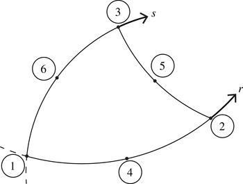
Nodal points in the isoparametric plane: 1–6 are used for the
 $P2$
element, 1–3 are used for
 $P1$
element.

We discretize the Galerkin formulation by using isoparametric triangular elements (Bathe Reference Bathe1996, figure 5.11) for the solution variables: figure 15 shows a representative element in the isoparametric domain with the corresponding node numbering. The velocity components are represented by the values at the six nodes per element (1–6 in figure 15) and interpolated using quadratic polynomials (
 $P2$
element), pressure is represented by the three corner nodes (1–3 in figure 15) and interpolated using a linear polynomial (
 $P1$
element). This choice of
 $P2$
–
 $P1$
element satisfies the Ladyzhenskaya–Babuška–Brezzi stability condition (Johnson Reference Johnson2009, p. 232).
The quadratic interpolation for the velocity components are defined as follows (with
 $r$
and
 $s$
defined in figure 15):
 $$\begin{eqnarray}\displaystyle & \displaystyle h_{1}^{q}(r,s)=1-3r-3s+2r^{2}+4rs+2s^{2}, & \displaystyle\end{eqnarray}$$
 $$\begin{eqnarray}\displaystyle & \displaystyle h_{2}^{q}(r,s)=-r+2r^{2}, & \displaystyle\end{eqnarray}$$
 $$\begin{eqnarray}\displaystyle & \displaystyle h_{3}^{q}(r,s)=-s+2s^{2}, & \displaystyle\end{eqnarray}$$
 $$\begin{eqnarray}\displaystyle & \displaystyle h_{4}^{q}(r,s)=4r-4rs-4r^{2}, & \displaystyle\end{eqnarray}$$
 $$\begin{eqnarray}\displaystyle & \displaystyle h_{5}^{q}(r,s)=4rs, & \displaystyle\end{eqnarray}$$
 $$\begin{eqnarray}\displaystyle & \displaystyle h_{6}^{q}(r,s)=4s-4rs-4s^{2}. & \displaystyle\end{eqnarray}$$
 $$\begin{eqnarray}\displaystyle & \displaystyle h_{1}^{l}(r,s)=1-r-s, & \displaystyle\end{eqnarray}$$
 $$\begin{eqnarray}\displaystyle & \displaystyle h_{2}^{l}(r,s)=r, & \displaystyle\end{eqnarray}$$
 $$\begin{eqnarray}\displaystyle & \displaystyle h_{3}^{l}(r,s)=s. & \displaystyle\end{eqnarray}$$
 $$\begin{eqnarray}\displaystyle & \displaystyle u(r,s)=\mathop{\sum }_{i=1}^{6}h_{i}^{q}u_{i}, & \displaystyle\end{eqnarray}$$
 $$\begin{eqnarray}\displaystyle & \displaystyle v(r,s)=\mathop{\sum }_{i=1}^{6}h_{i}^{q}v_{i}, & \displaystyle\end{eqnarray}$$
 $$\begin{eqnarray}\displaystyle & \displaystyle p(r,s)=\mathop{\sum }_{i=1}^{3}h_{i}^{l}p_{i}. & \displaystyle\end{eqnarray}$$
 $h_{i}^{q}$
,
 $h_{i}^{l}$
are quadratic and linear interpolations;
 $u_{i}$
,
 $v_{i}$
and
 $p_{i}$
are the corresponding nodal values. Subscripts denote the nodal points shown in figure 15.
The unit tangent vector in the
 $xOy$
is computed by
 $$\begin{eqnarray}\displaystyle \boldsymbol{t}=\frac{\displaystyle \mathop{\sum }_{i=1}^{3}s_{i}\frac{\text{d}h_{i}^{q}}{\text{d}s}}{\displaystyle \left\Vert \mathop{\sum }_{i=1}^{3}s_{i}\frac{\text{d}h_{i}^{q}}{\text{d}s}\right\Vert }, & & \displaystyle\end{eqnarray}$$
with
 $s_{i}$
being nodal position vector and
 $\text{d}h_{i}^{q}/\text{d}s$
being a scalar corresponding to the element edge over which the computation is carried out. The normal component is found simply by
 $\boldsymbol{n}=\boldsymbol{k}\times \boldsymbol{t}$
. The coordinates are interpolated with the quadratic interpolation functions:
 $$\begin{eqnarray}\displaystyle & \displaystyle x(r,s)=\mathop{\sum }_{i=1}^{6}h_{i}^{q}x_{i}, & \displaystyle\end{eqnarray}$$
 $$\begin{eqnarray}\displaystyle & \displaystyle y(r,s)=\mathop{\sum }_{i=1}^{6}h_{i}^{q}y_{i}, & \displaystyle\end{eqnarray}$$
 $x_{i}$
and
 $y_{i}$
are the coordinates of the node points in the element and
 $h_{i}^{q}$
is defined in (A 14). Because the computations are performed in the isoparametric domain, we need to express the mapping for the derivatives from the
 $xOy$
plane to the isoparametric plane, which is given by
 $$\begin{eqnarray}\displaystyle \left[\begin{array}{@{}c@{}}\displaystyle \frac{\unicode[STIX]{x2202}}{\unicode[STIX]{x2202}x}\\ \displaystyle \frac{\unicode[STIX]{x2202}}{\unicode[STIX]{x2202}y}\end{array}\right]=J^{-1}\left[\begin{array}{@{}c@{}}\displaystyle \frac{\unicode[STIX]{x2202}}{\unicode[STIX]{x2202}r}\\ \displaystyle \frac{\unicode[STIX]{x2202}}{\unicode[STIX]{x2202}s}\end{array}\right]. & & \displaystyle\end{eqnarray}$$
Jacobian (
 $J$
) of the transformation in (A 22) is given by
 $$\begin{eqnarray}\displaystyle J=\left[\begin{array}{@{}cc@{}}\displaystyle \frac{\unicode[STIX]{x2202}x}{\unicode[STIX]{x2202}r} & \displaystyle \frac{\unicode[STIX]{x2202}y}{\unicode[STIX]{x2202}r}\\ \displaystyle \frac{\unicode[STIX]{x2202}x}{\unicode[STIX]{x2202}s} & \displaystyle \frac{\unicode[STIX]{x2202}y}{\unicode[STIX]{x2202}s}\end{array}\right]. & & \displaystyle\end{eqnarray}$$
We use Gauss quadrature to carry out the integrations. Plane integrations are evaluated over triangles using a seven-point Gauss integration rule (Bathe Reference Bathe1996, §§ 5.5.4 and 5.5.5).
 $r$
and
 $s$
are evaluated at the Gauss points of integration over triangles. Boundary integrals are evaluated using a three-point Gauss integration rule (Bathe Reference Bathe1996, § 5.5.3). In both cases, the Gauss quadrature integrates exactly polynomials of order at most 5. The highest-order polynomial in the integrations is four, therefore the integrations are exact throughout the numerical method.
After forming the element matrix
 $\unicode[STIX]{x1D63C}^{k}$
and right-hand side vector
 $\boldsymbol{R}^{k}$
over each element
 $e^{k}$
for the unknowns by using (A 9)–(A 11), we form a global stiffness matrix
 $\unicode[STIX]{x1D63C}$
and right-hand side vector
 $\boldsymbol{R}$
. We impose constraints on certain solution variables with the use of Lagrange multiplier method: we extend the solution vector by adding the Lagrange multipliers
 $\unicode[STIX]{x1D706}$
for the constraints and extending the system of equations to
 $$\begin{eqnarray}\displaystyle \left[\begin{array}{@{}cc@{}}\unicode[STIX]{x1D63C} & \boldsymbol{n}_{i}^{\text{T}}\\ \boldsymbol{n}_{i} & 0\end{array}\right]\left[\begin{array}{@{}c@{}}\boldsymbol{u}\\ \unicode[STIX]{x1D706}\end{array}\right]=\left[\begin{array}{@{}c@{}}\boldsymbol{R}\\ u_{i}^{\ast }\end{array}\right], & & \displaystyle\end{eqnarray}$$
where
 $\boldsymbol{n}_{i}$
is a vector with all entries equal to zero, but its
 $i$
th entry which is equal to one,
 $u_{i}^{\ast }$
is the imposed constraint at node
 $i$
.