

I. INTRODUCTION
With the multiplication and miniaturization of telecommunications systems and their integration in restricted environments, such as smart-phones, tablets, cars, airplanes, and other embedded systems. The design of compact multi-band and broadband antennas with high gains and a good efficiency becomes a necessity.
For designing this kind of antennas, a lot of techniques are used:
(1) designing multi-band antennas operating in several frequencies bands. Several studies have been made to design this kind of antennas using fractal geometries or adding slots to the radiating elements [Reference Mehdipour and Trueman1–Reference Reha and Oulad Said7].
(2) designing UWB antennas operating in the frequencies bands exceeding 500 MHz or having a fractional bandwidth of at least 0.20. The UWB wireless communication occupies a bandwidth from 3.1 to 10.6 GHz (based on the FCC “Federal Communication Commission”) [Reference Liqin, Jin and Chonghua8–Reference Oppermann, Hämäläinen and et Iinatti17].
(3) designing antennas with a broad-band behavior, a high gain, and a good efficiency using some special materials [Reference Habib Ullah, Islam and Mandeep18–Reference Chun-Yin, Shih-Huang and Tzu-Hao21].
One of the interesting techniques used to design miniaturized antennas with multi-band and broad band behavior is the fractal geometry, because it is a simple technique based on the auto-similarity, the most known techniques used are: MINKOWSKI, KOCH, Tree, HILBERT, SIERPINSKI, APOLLONIUS circles, CANTOR Set… [Reference Balanis16, Reference Chen, Wang and Hsu22, Reference Jeemon, Shambavi and Alex23].
In this paper, we study the behavior of a coplanar waveguide (CPW)-fed H-tree fractal slot antenna versus the iteration numbers. The simulation is done by FEKO 6.3 based on the method of the moment (MoM) [24]. The measurements are done by the HP 8719C 50 MHz-13.5 GHz Network Analyzer.
II. LITTERATURE REVUE OF THE TREE FRACTAL ANTENNAS
A) The generation of Tree fractal geometry
To generate this kind of fractal structure, we apply the following steps:
(1) For the initiator or “iteration 0”, the structure has three branches, the vertical one is the “parent” the two others are the “Childs” with an inclination (θ).
(2) At each iteration, the same shape is generated with a reduction factor “h” (Fig. 1).
The three first iterations of the Tree fractal structure.

In the fractal structures, we use another dimension concept known as “the Hausdorff dimension” which defined by the equation (1) [Reference Mandelbrot25, Reference Falconer26].
 $$d=\displaystyle{{{\rm ln\lpar }n\rpar } \over {{\rm ln\lpar }R\rpar }}\comma \;$$
where the fractal is formed of “n” copies whose size has been reduced by a factor of “R”.
For the Tree structure, if the reduction factor R = 2, the Hausdorff dimension is given by the equation (2).
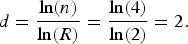 $$d=\displaystyle{{{\rm ln\lpar }n\rpar } \over {{\rm ln\lpar }R\rpar }}=\displaystyle{{{\rm ln\lpar 4\rpar }} \over {{\rm ln\lpar 2\rpar }}}=2.$$
B) The generation of H-tree fractal geometry
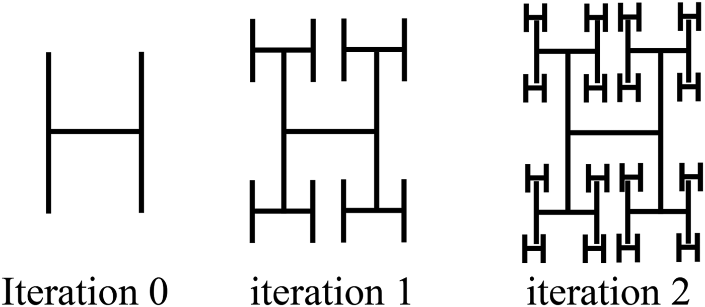
The H-tree geometry is a modified Tree geometry with the same concept (Fig. 2). The initiator is a structure like the letter “H”. On each iteration, we create four copies of the previous iteration with a reduction factor “R”.
The three first iterations of the H-tree fractal structure.
For the H-tree structure, if the reduction factor R = 2, the Hausdorff dimension is given by the equation (3).
 $$d=\displaystyle{{{\rm ln\lpar }n\rpar } \over {{\rm ln\lpar }R\rpar }}=\displaystyle{{{\rm ln\lpar 4\rpar }} \over {{\rm ln\lpar 2\rpar }}}=2.$$
C) The use of the Tree fractal on the design of the antennas
The Tree Fractal structures are used in many works for the antennas design with good performances.
In 1986, according to our investigations, KIM has published the first paper on Fractal geometries antennas [Reference Kim and Jaggard27]. In 1999, WERNER studied the effect of the number of iterations on the behavior of fractal antennas in general and in particular of the tree structures [Reference Werner, Haupt and Werner28]. In 2004, PETKO studied the 3D-Tree fractal antennas and found out the relationship between the geometry parameters and the performances of this kind of fractal structures [Reference Petko and Werner29]. In 2009, He studied the array of Tree fractal antennas and he demonstrated that we can have better results with this technique [Reference Petko and Werner30]. In 2011, POURAHMADAZA created modified patch antennas fed by microstrip lines and having the shape of “PYTHAGORE TREE”. He demonstrated that by increasing the number of iterations we can have miniaturized antennas with more resonance frequencies, an ultra wideband behavior, good efficiency, and better matching [Reference Pourahmadazar, Ghobadi and Nourinia31]. In 2013, DUMOND studied experimentally the Random 2D-Tree fractal antennas and he demonstrated that with this kind of structures, we can have antennas with good performances, multi-band and UWB behavior [Reference Dumond, Khelloufi and Allam32]. Also, NASER-MOGHADASI has introduced a miniaturized Tree fractal structure operational for all the UWB applications, he also set up parasite elements in order to eliminate some frequencies bands [Reference Naser-Moghadasi, Sadeghzadeh, Sedghi, Aribi and Virdee33]. VARADHAN proposed a tri-bands Tree fractal antenna for the radio frequency identification (RFID) applications [Reference Varadhan, Pakkathillam, Kanagasabai, Sivasamy, Natarajan and Palaniswamy3]. LIU proposed another structure with a high gain for the UHF-RFID, this antenna is composed of a traditional patch and another layer composed of a four Tree fractal elements [Reference Liu, Xu and Wu34].
In the next section, three iterations of a CPW-fed H-tree antenna will be simulated and measured.
III. ANTENNA DESIGN
To design the first iteration of CPW H-tree structure, we start from the first iteration of a CPW tree fractal antenna designed by VARADHAN [Reference Varadhan, Pakkathillam, Kanagasabai, Sivasamy, Natarajan and Palaniswamy3]; this structure is a tri-band antenna with three resonant frequencies f r1 = 3.6 GHz, f r2 = 5.8 GHz, and f r3 = 8.2 GHz.
After that, we modify this structure to have an H-tree structure (θ = π/2). Figure 3 shows the difference between the S 11 parameters of the Tree and the H-tree structures.
The S 11 parameter versus the frequency for the H-tree and the tree structures.
We observe that the modified structure is a bi-band antenna with two resonant frequencies f r1 = 5.8 GHz and f r2 = 8.1 GHz. Also, the simulated gain and the −10 dB bandwidth of the H-tree structure are very important. Table 1 shows the difference between the gains of the two structures for two frequencies 5.8 and 8.2 GHz.
The difference between the gains.

In the following, we will analyze the behavior of three iterations of the H-tree structure.
As shown in Fig. 4, the proposed antenna is printed on a FR4 dielectric substrate of relative permittivity ε r = 4.3, thickness H = 1.6 mm, loss tangent 0.025 and fed by a CPW transmission line with a signal strip width S 0 and a gap distance G between the signal strip and the ground plane. Several studies have used this mode of feeding because it is one of the techniques to increase the bandwidth of the antennas [Reference Zhou, Wang, Wang, Zong and Ma4, Reference Reha and Bouchouirbat6, Reference Kumar and Sawant10].
The geometry of the CPW-fed H-tree Fractal Antenna.
For a reduction factor R = 2, the generation of the different iterations of the H-tree Fractal antenna (Fig. 5) is based on a simple formula (4):
The three iterations of the H-tree fractal Antenna.
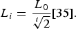 $${L_i}=\displaystyle{{{L_0}} \over {\root i \of 2 }}[35].$$
The other parameters are as follow:
W = 40 mm, L = 40 mm, B = 4, G = 0.5 mm, L 0 = 20 mm, and S 0 = 0.8 mm.
A parametric study is based on the variation of the parameter S.
All the simulations and the measurements are done in the band of 3.1–10.6 GHz.
IV. RESULTS AND DISCUSSIONS
A) The first iteration
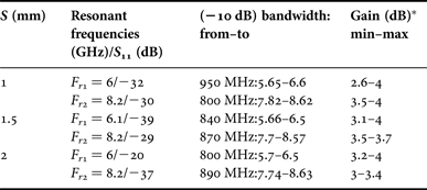
For the first iteration of the CPW-fed H-tree fractal antenna, the variation of simulated S 11 parameter versus the frequency for some values of S is shown in Fig. 6. Table 2 summarizes for each value of S, the resonant frequencies, the S 11 values on the resonant frequencies, the −10 dB bandwidths, the maximum and minimum gains.
Simulated S 11 versus frequency graph of the antenna (first iteration).
Simulated bandwidths and the gains for the antenna (first iteration).
*The gain is simulated on the (−10 dB) bandwidth.
We note that for this first iteration, the simulated structures are dual-band antennas with two resonant frequencies and all the bandwidths exceed 500 MHz.
The antenna with the parameter S = 2 is manufactured and measured. Figure 7 shows the comparison between simulated and measured S 11 parameter. Figure 8 shows the 3D-Total Gain pattern of the antenna for the frequencies 5.8 and 8.2 GHz.
Simulated and measured S 11 versus frequency graph of the antenna (first iteration).
the 3D Total Gain pattern for the frequencies 5.8 and 8.2 GHz. (a) f = 5.8 GHZ (maximum gain = 4 dB) (b) f = 8.2 GHZ (maximum gain = 3.4 dB).
In comparison with the Three-band CPW-fed tree fractal antenna designed by VARADHAN [Reference Varadhan, Pakkathillam, Kanagasabai, Sivasamy, Natarajan and Palaniswamy3], the proposed CPW-fed H-tree fractal antenna is a dual-band antenna for the 5.8 and 8.2 GHz RFID applications, and its gain is much better. This structure is also a good solution for the 5.9 GHz wireless local area networks (WLAN) IEEE802.11p, a part of 5 GHz WLAN IEEE 802.11 1/h/j/n/ac and 5.8 GHz worldwide interoperability for microwave access system (WIMAX) IEEE802.16 applications.
B) The second iteration
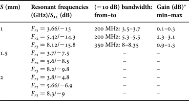
For the second iteration of the CPW-fed H-tree fractal antenna, the variation of simulated S 11 parameter versus the frequency for some values of S is shown in Fig. 9. Table 3 summarizes for each value of S, the resonant frequencies, the S 11 values on the resonant frequencies, the −10 dB bandwidths, the maximum and minimum gains.
Simulated S 11 versus frequency graph of the antenna (second iteration).
Simulated bandwidths and the gains for the antenna (second iteration).
*The gain is simulated on the (−10 dB) bandwidth.
We note that for this second iteration, the simulated structures are tri-band antennas with three resonant frequencies.
The antenna with the parameter S = 1 is manufactured and measured. Figure 10 shows the comparison between the simulated and the measured S 11 parameter. Figure 11 shows the 3D-Total Gain pattern of the antenna for the frequencies 5.3 and 8.3 GHz.
Simulated and measured S 11 versus frequency graph of the antenna (second iteration).
the 3D Total Gain pattern for the frequencies 5.3 and 8.3 GHz. (a) f = 5.3 GHZ (maximum gain = 3.1 dB) (b) f = 8.3 GHZ (maximum gain = 1.3 dB).
This antenna is a good solution for 3.6 GHz WLAN IEEE802.11y, 3.6 and 8.2 GHz RFID, 5.4 GHz HiperLAN, and C-band applications.
C) The third iteration
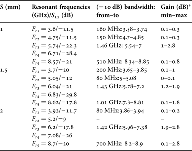
For the third iteration of the CPW-fed H-tree fractal antenna, the variation of simulated S 11 parameter versus the frequency for some values of S is shown in Fig. 12. The Table 4 summarizes for each value of S, the resonant frequencies, the S 11 values on the resonant frequencies, the −10 dB bandwidths, the maximum, and minimum gains.
Simulated S 11 versus frequency graph of the antenna (third iteration).
Simulated bandwidths and the gains for the antenna (second iteration).
*The gain is simulated on the (−10 dB) Bandwidth.
We note that for this third iteration, the simulated structures are tetra-band antennas with 5 resonant frequencies and some of the bandwidths exceed 1.4 GHz.
The antenna with the parameter S = 1 is manufactured and measured. Figure 13 shows the comparison between the simulated and the measured S 11 parameter. We observe that the measurement is different to the simulation. Such a difference between the simulation and experimental results can probably be ascribed to the fabrication imperfections (like inaccuracy in the milling and etching processes and connector soldering).
Simulated and measured S 11 versus frequency graph of the antenna (third iteration).
Figure 14 shows the 3D-Total Gain pattern of the antenna for the frequency 6 GHz.
the 3D Total Gain pattern for the frequency 6 GHz (maximum gain = 2.8 dB).
This antenna is a good solution for 3.6 GHz WLAN IEEE802.11y, 3.6 and 5.8 GHz RFID, 5.8 GHz WIMAX IEEE802.16, 5.9 GHz WLAN IEEE 802.11p, and C-band applications.
V. CONCLUSION
The fractal concept is a one of the better solutions to design miniaturized broadband and multi-band antennas. The use of the CPW-fed technique increases the bandwidth of the antennas, and it is very easy to manufacture because the antenna is designed on one face of a printed circuit board (PCB).
Increasing the number of iteration of the CPW-fed H-tree fractal antenna allows obtaining a low profile antenna with a multi-band and broadband behavior.
For some configurations of the proposed structures, the antennas operate in many applications, such as WLAN IEEE802.11 a/h/j/n/ac/y, WIMAX IEEE802.16, RFID, C-BAND, HiperLAN, and UWB applications.
Also, more refinement can be done to obtain antennas with better performances and good matching.
ACKNOWLEDGEMENT
All authors would like to thank Telecoms laboratory of Royal Air Academy and Electronic Laboratory of IGA-MARRAKECH for providing support and assistance to perform measurements.
Abdelati Reha was born in Casablanca-Morocco in 1975, he received his degree of engineer in Aeronautic from the Royal Air Academy of Marrakech-Morocco in 1999, and the degree of engineer in Telecommunication from the INPT-Rabat-Morocco in 2002. He is currently working toward Ph.D. degree at RITM Laboratory in ESTC – Hassan II University – Casablanca-Morocco. His main research interests are in fractal antennas, UWB applications
Dr. Abdelkebir Elamri received his Ph.D. in Signals and Systems at the University of Montpellier 1990 (France). Currently, a professor in the Electrical Engineering Department at the School of Technology Casablanca (ESTC). He is a member of the laboratory Radio Telecommunications (RITM). His research interests in the characterization, modeling of antennas for applications in telecommunications, radar, and mobile radio.
Dr. Othmane Benhmammouch was born in Mohammedia, Morocco, in 1982. He received his Master in Computer-sciences from Université de Versailles, Versailles, France, in 2005 and Master in Applied Mathematics from the Ecole Normale Supérieure de Cachan (ENS Cachan), Cachan, France, in 2006. He received his Ph.D. in Electronic Engineering from Université de Bretagne Occidentale, Brest, France, in 2011. He joined, for 2 years, Ecole Nationale des Sciences Cognitives (ENSC-IPB), Bordeaux, France, in 2010, where he was an Assistant Professor. In 2012, he joined the Centre Scientifique et Technique du Batimrent (CSTB), Nantes, France as a postdoctoral researcher and works in EMW propagation prediction in Telecommunications. Since September 2013 he has been with Mundiapolis University, Casablanca, Morocco, where he is currently a professor. His main research interests include EMW propagation prediction, fractal antennas, antennas design, and numerical analysis.
Dr. Ahmed Oulad Saïd was born in Tetouan (Morocco) in 1961. He received the license degree in Physics in 1983 from the Faculty of Sciences of Rabat; he received the DEA in Instrumentation and Measurements from the University of Bordeaux I France in 1984. In 1987, he received Ph.D. degree in microwave at the University of Bordeaux I France. He is the head of Electrical and Telecommunications Department in the Royal Air Academy. His main research interests are in fractal antennas, UWB applications, microwaves, MIMO antennas, optical fibers. He is the head of the Association of Modeling and Simulation in the Enterprises – Section Morocco (AMSE).
Dr. Abdelhakim El Ouadih was born in Casablanca-Morocco in 1976, he received his degree of engineer in Aeronautic from the Royal Air Academy of Marrakech-Morocco in 1999, degree of engineer in Telecommunication from the INPT-Rabat-Morocco in 2002, master's degree of Telecommunication from Kadi Ayyad University, Marrakech-Morocco, and Ph.D. degree in Telecommunication from Kadi Ayyad University, Marrakech-Morocco. He is currently a professor in the Royal Air Academy, Marrakech-Morocco. His main research interests are in antennas, propagation, and wireless communication.
 Marouane Bouchouirbat was born in Marrakech-Morocco in 1986, he received his degree of Engineer in the high institute of Applied Engineering of Marrakech-Morocco in 2012. He is a professor in the IGA-MARRAKECH. His main research interests are in automation, telecommunication, and electric systems.