A. Measuring Flow Diversification

Because investor-level daily flows are unavailable, we use share-class flows to proxy for co-movement in investor liquidity demands. This approach relies on the fact that share classes segment investors by distribution channel and account type, and prior work documents systematic differences across retail, retirement, broker-sold, and institutional investors.Footnote ⁶ We exploit this systematic variation in liquidity demands across share classes in measuring flow diversification. We first define flows for share class k in fund i at time t as

(1) $$ {Flows}_{i,k,t}={TNA}_{i,k,t}-{TNA}_{i,k,t-1}\times \left(1+{r}_{i,k,t}\right), $$

where TNA represents total net assets and r is the net return after fees.Footnote ⁷ Aggregating flows across all k share classes yields net flows for fund i at time t:

(2) $$ {Flows}_{i,t}=\sum \limits_{k=1}^K{Flows}_{i,k,t}. $$

Our measure of flow diversification, FlowCorr, is based on the covariance of flows across share classes. Intuitively, FlowCorr captures the extent to which liquidity demands across investor groups move together, conditional on a given level of fund net flows. We compute FlowCorr as the average pairwise cross-product of value-weighted deviations of class-level flows from fund-level net flows, scaled by the average squared value-weighted deviation across all share classes. This ensures that FlowCorr is comparable across funds with different numbers of share classes:

(3) $$ {\displaystyle \begin{array}{c}{FlowCorr}_{i,t}=\frac{\sum \limits_{k\ne l}\mathit{\operatorname{cov}}\left({flows}_{i,k,t},{flows}_{i,l,t}\right)}{\mathit{\operatorname{var}}\left({flows}_{i,k,t}\right)}\\ {}=\frac{\frac{2}{K\left(K-1\right)}\sum \limits_{k=1}^{K-1}\sum \limits_{j=k+1}^K\left[{w}_{k,t-1}\left({Flows}_{i,k,t}-{Flows}_{i,t}\right)\times {w}_{j,t-1}\left({Flows}_{i,j,t}-{Flows}_{i,t}\right)\right]}{\frac{1}{K}\sum \limits_{k=1}^K{w}_{k,t-1}^2{\left({Flows}_{i,k,t}-{Flows}_{i,t}\right)}^2},\end{array}} $$

where $ {w}_{k,t-1}=\frac{TNA_{i,k,t-1}}{TNA_{i,t-1}} $ is the weight of share class k in fund i at time t − 1. FlowCorr is bounded between −1 and +1, and positive (negative) values indicate positively (negatively) correlated flows across share classes.

FlowCorr reflects both a clientele effect, the correlation in liquidity needs across types of investors segmented by share classes, and a client effect, which captures idiosyncratic, uncorrelated liquidity demands across individual investors. Clientele effects are likely endogenous because fund managers understand the typical liquidity needs of investors in different share classes, such as periodic retirement contributions and distributions, 401(k) rebalancing, and advance notice from institutional clients. These predictable features generate a slow-moving component in FlowCorr that shifts primarily when funds alter their clientele structure by adding or removing share classes.Footnote ⁸ In contrast, the client effect arises from unpredictable variation in investors’ liquidity needs that lies outside managerial control.

To separate these forces, we extract the average (permanent) component of FlowCorr using a backward-looking 60-day moving average (MA) process, interpreting it as the conditional expectation of FlowCorr from clienteles. Deviations from the average represent the idiosyncratic, unpredictable correlation in liquidity needs across investors. We denote these components ExpFlowCorr and UnexpFlowCorr, respectively. Importantly, this decomposition is not intended as a statistical forecasting model. Instead, it provides a parsimonious way to separate predictable liquidity patterns that managers can internalize from deviations from the average that cannot be managed ex ante. Unexpected flow correlation may still be correlated with unobserved market, investor demand, or fund-level shocks. Accordingly, we interpret UnexpFlowCorr as a measure of synchronized liquidity needs that moderates the effect of unexpected outflows on future fund returns, rather than a fully exogenous shock.

B. Data and Sample

We use the Morningstar Mutual Fund Database, which provides daily data on flows and returns for 7,489 funds at the share class level. Morningstar receives daily data on NAVs, assets, and returns through direct feeds from fund managers, fund administrators, custodians, trusts, advisors, and fund companies. To construct our sample, we start with all U.S.-domiciled open-end equity mutual funds in the database. We exclude index funds because they attract a particular type of clientele and because Vanguard, the largest index fund provider, does not provide daily flow data to Morningstar. The sample period spans January 2007 through December 2024.

We supplement daily flow data with additional information on fund characteristics (i.e., expenses, turnover, load, and age) from the CRSP survivorship-bias-free Mutual Fund database. To merge Morningstar with CRSP, we first match on CUSIP. When CUSIP is unavailable, we use TICKER, and if neither identifier is available (representing 13% of the sample), we manually match observations using fund and share-class names. After matching, our sample consists of 6,548 funds and 22,076 share classes. At the end of 2024, our sample represents approximately 60% of total assets in active U.S. equity mutual funds. We extract equity style classifications from Morningstar along with their benchmark returns. We aggregate reported variables across share classes at the fund level by value weighting them using lagged total net assets (TNA) of each share class. The average fund in our sample has 4.17 share classes, with more than 91% of funds reporting daily observations for at least two share classes.

To determine clienteles, we map share classes into three categories used by Morningstar and other practitioners: i) retail, ii) retirement, and iii) advisor/institutional, hereafter referred to simply as institutional. We merge institutional and advisor share classes into one group because, in practice, fund families use these labels interchangeably. To do this, we start with the existing Morningstar mappings, but for share classes not categorized by Morningstar, we rely on CRSP classifications.Footnote ⁹ At the end of 2024, the percentages of aggregate assets corresponding to retail, retirement, and institutional groups are 21%, 18%, and 61%, respectively.

C. Descriptive Statistics

Definitions for key variables of interest appear in the Appendix. With exceptions noted later, most tests are based on the sample of fund-days with net outflows, measured after aggregating flows across all share classes. This is because i) trading costs associated with inflows are borne by both entering and incumbent shareholders, ii) the literature described earlier largely focuses on externalities generated by outflows, and iii) it is relatively inexpensive to equitize inflows in the futures market and then minimize trading costs by slowly purchasing target securities. Descriptive statistics for the outflow-only sample are provided in Table A1.

The average FlowCorr in the sample is only 0.20, but its standard deviation is more than twice as large. Given the MA filter used in the decomposition, it is not surprising that the standard deviation of ExpFlowCorr is close to its mean (0.16 compared to 0.19), but that the standard deviation of UnexpFlowCorr is much higher than its mean (0.39 compared to 0.01). Although UnexpFlowCorr is transitory by construction, it is precisely these short-lived deviations that generate immediacy demands, making them economically relevant. The cross-sectional average autocorrelation of FlowCorr is 0.10 based on the full sample of all fund days. Also of interest is the distribution of cash buffers, particularly in the context of expected flow correlation. The average cash buffer (Cash), defined as the sum of cash and cash equivalents scaled by total assets, is 3.97%.Footnote ¹⁰ But the standard deviation is more than twice the mean (9.42%), and the median is 1.83%, implying active management of cash levels.

A. Determinants of Flow Correlation

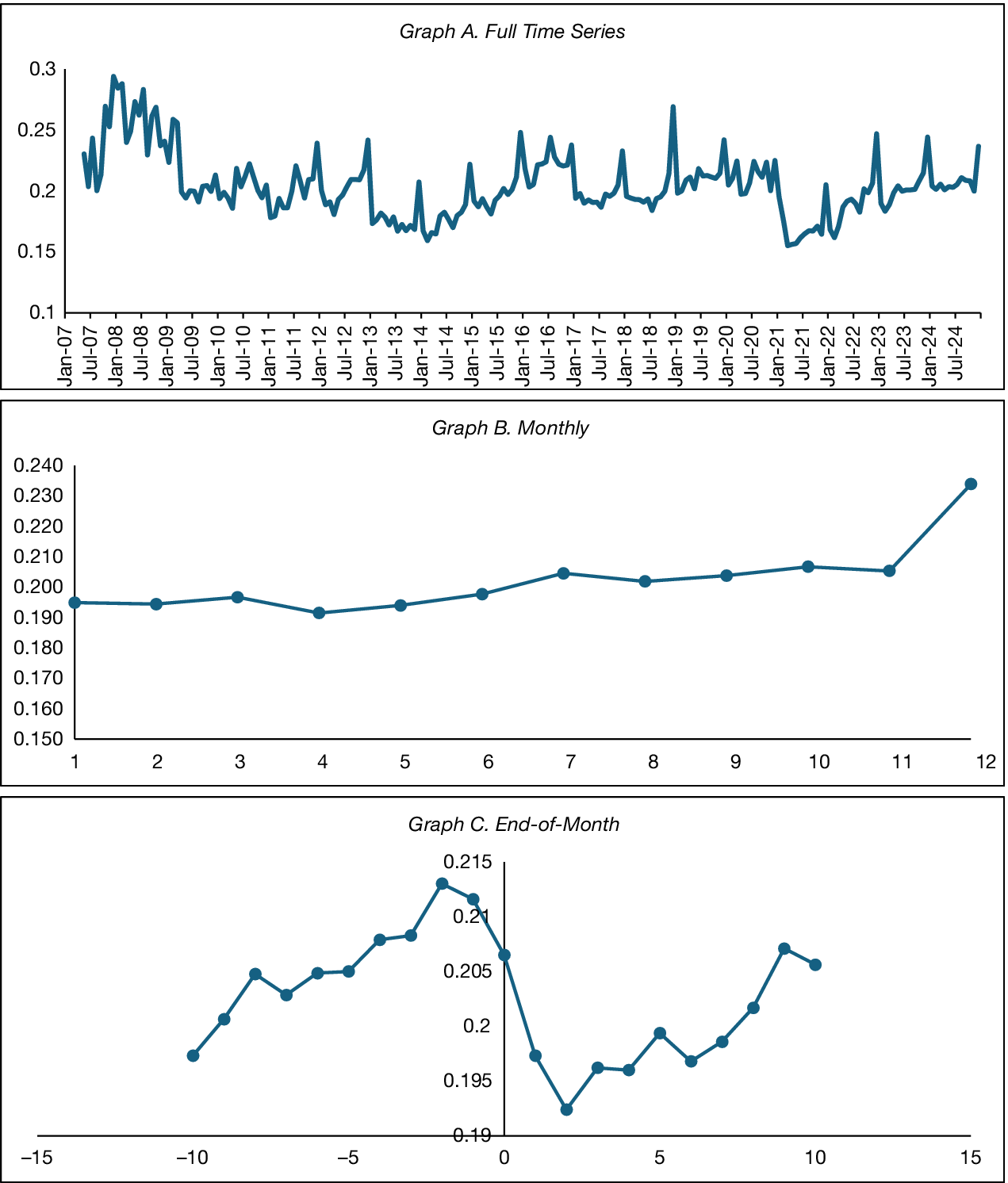
We start by examining the determinants of flow correlation. Since our purpose is to broadly understand flow correlation, we use the full panel of fund-day observations, including days with net inflows and outflows. Graph A of Figure 1 shows monthly average FlowCorr over the sample period. The long-run average is 0.20 with elevated values during the financial crisis (2008–2009) and other common liquidity shocks. Interestingly, each of the local peaks in the graph corresponds to December. Graph B plots monthly averages and confirms the notable increase in flow correlation in December, consistent with end-of-year portfolio rebalancing and tax-motivated trading by investors. Graph C shows daily flow correlations from 10 days before to 10 days after the end of the month, where day 0 is the last trading day of the month. There is a striking increase in flow correlations 2 days before the last trading day of the month, consistent with a systematic liquidity demand related to the monthly payment cycle termed “dash for cash” by Etula et al. (Reference Etula, Rinne, Suominen and Vaittinen2020). Collectively, Graphs B and C imply that flow correlation responds systematically to recurring calendar-based liquidity demands.

FIGURE 1Time-Series Patterns in Flow Correlation

Graph A of Figure 1 plots the monthly average daily flow correlation from January 2007 to December 2024. Graph B reports the average daily flow correlation in each calendar month. Graph C contains the average daily flow correlation from 10 trading days before to 10 trading days after the end of the month (day 0 denotes the last trading day of the month).

FIGURE 1 Long description

A three-panel set of line graphs.

Graph A, titled Full Time Series, plots monthly average daily flow correlation from January 2007 to December 2024. The X-axis shows years in six-month increments. The Y-axis ranges from 0.1 to 0.3. The data shows a volatile trend that peaks near 0.3 in early 2008, followed by a general decline and stabilization between 0.15 and 0.25, with periodic spikes occurring annually.

Graph B, titled Monthly, shows average daily flow correlation by calendar month. The X-axis is labeled 1 through 12. The Y-axis ranges from 0.150 to 0.240. The line remains relatively flat between 0.190 and 0.200 from months 1 to 6, then shows a steady upward trend starting in month 7, reaching a peak of approximately 0.235 in month 12.

Graph C, titled End-of-Month, displays correlation from 10 trading days before to 10 trading days after the end of the month. The X-axis ranges from -15 to 15, with 0 marking the last trading day. The Y-axis ranges from 0.19 to 0.215. The data shows a sharp increase starting at day -10, peaking at day -2 at approximately 0.213, followed by a steep decline to a trough of 0.192 at day 2, before recovering toward 0.205 by day 10.

A formal regression analysis appears in Table 1. The dependent variable is FlowCorr on day t, and the independent variables capture the degree to which flow correlation is related to fund-specific attributes, responds to time-varying market conditions, and reflects changes in investor heterogeneity. Column 1 includes fund fixed effects that control for unobservable, time-invariant fund characteristics. Column 2 additionally includes style-quarter fixed effects to absorb any liquidity shocks that may be clustered within each style and quarter. Robust standard errors, clustered at the fund-quarter level, appear in parentheses. We do not include cash holdings as a control in these regressions because cash holdings are a managerial response to predictable liquidity risk (see discussion in Section V.A).

TABLE 1Determinants of Flow Diversification

TABLE 1 Long description

The table presents regression results for six models. The dependent variable is FlowCorr.

Independent variables and their coefficients (standard errors in parentheses):

* Log (Fund size): -0.004*** (0.001) in models 1, 3, 5; -0.003*** (0.001) in models 2, 4, 6.

* Expense ratio: 0.027*** (0.004) in models 1, 3, 5; 0.045*** (0.005) in models 2, 4, 6.

* Turnover: -0.006* (0.003) in models 1, 3, 5; -0.005* (0.003) in models 2, 4, 6.

* Std. Dev. (Flow sub t minus 2, t): 0.011*** (0.002) across all models.

* Log (Age): -0.011*** (0.001) in models 1, 3, 5; -0.027*** (0.002) in models 2, 4, 6.

* Load: -0.002 (0.144) in models 1, 3, 5; 0.577*** (0.166) in models 2, 4, 6.

* Flow-perf. sensitivity: 0.000 (0.003) in models 1, 3, 5; 0.003 (0.003) in models 2, 4, 6.

* R m sub t: -0.025** (0.011) in models 1, 3, 5; -0.023** (0.011) in models 2, 4, 6.

* R m sub t minus 3, t minus 1: -0.086*** (0.009) in models 1, 3, 5; -0.084*** (0.008) in models 2, 4, 6.

* Sentiment: -0.016*** (0.005) in models 1, 3, 5; -0.023*** (0.005) in models 2, 4, 6.

* December indicator: 0.036*** (0.001) in models 1, 3, 5; 0.034*** (0.001) in models 2, 4, 6.

* Month-end indicator: 0.008*** (0.001) in models 1, 3, 5; 0.007*** (0.001) in models 2, 4, 6.

* Share class increase indicator: -0.021*** (0.005) in model 3; -0.019*** (0.005) in model 4.

* Retail class increase indicator: -0.035*** (0.009) in model 5; -0.032*** (0.009) in model 6.

* Institutional class increase indicator: -0.024*** (0.006) in model 5; -0.022*** (0.006) in model 6.

* Retirement class increase indicator: -0.019 (0.016) in models 5 and 6.

* Constant: 0.255*** (0.020) in models 1, 3, 5; 0.240*** (0.020) in models 2, 4, 6.

Fixed Effects (F E):

* Fund F E: Yes for all models.

* Style-quarter F E: Yes for models 2, 4, and 6.

Statistics:

* N: Approximately 8.17 million for all models.

* Adj-R super 2: 0.060 for models 1, 3, 5; 0.062 for models 2, 4, 6.

Using column 2, larger and older funds have significantly lower flow correlation, consistent with more established funds attracting broader and more heterogeneous investor bases: a 1-standard-deviation increase in fund size and age reduces flow correlation by 4.53% and 14.89%, respectively. By contrast, higher expense ratios and loads are associated with higher flow correlation, consistent with fee structures segmenting investors into more homogeneous clienteles; the corresponding effects are 9.83% and 2.80%, respectively. Higher turnover funds, which trade more frequently and likely attract shorter horizon or performance-sensitive investors, also exhibit more synchronous flows.

Market-level factors also matter. Contemporaneous and lagged market returns are negatively related to FlowCorr, consistent with declining markets generating redemptions across investors. The negative coefficient on sentiment is consistent with mutual fund flows reflecting investor sentiment (Frazzini and Lamont (Reference Frazzini and Lamont2008)) and sentiment shifts producing more correlated liquidity demands. The December and month-end indicators are both positive and highly significant, matching the spikes in Figure 1: flow correlation is almost 20% higher in December and 4% higher in the final trading days of the month. These results indicate that broad market conditions and recurring calendar effects contribute meaningfully to synchronized investor liquidity demands.

Columns 3 and 4 add an indicator equal to 1 when a new share class is introduced. The coefficient is −0.02, with a standard error of 0.005, implying a 10% reduction relative to the sample average FlowCorr of 0.20. Columns 5 and 6 separate retail, institutional, and retirement class additions. Retail and institutional additions substantially reduce flow correlation, suggesting that new distribution channels introduce investors with liquidity needs less synchronized with existing clienteles. Retirement class additions, which typically attract slow-moving contribution-driven flows, do not significantly affect flow correlation, perhaps because only 258 such additions occur in our sample.

B. Background Externalities and Prerequisites

A number of studies use monthly data to show that large outflows force mutual funds to engage in costly trading, generating an externality for non-redeeming shareholders. However, as discussed in Section II, redemption-driven trading occurs over the next few days (intra-month). We therefore replicate these findings in a daily setting to provide a benchmark for interpreting the economic significance of flow diversification. We form separate quintiles for outflows and inflows on day t and examine returns on t + 1, t + 2, and t + 3 and the cumulative return from t + 1 to t + 3. Panel A of Table A2 shows that the difference in t + 1 to t + 3 cumulative returns between small versus large outflow quintiles is 1.22 basis points, with a standard error that is one-third of that. In other words, funds experiencing larger outflows have lower subsequent returns. Panels B and C show that these return differences exist in both liquid and illiquid funds. As expected, return differences only exist for fund-days with outflows.

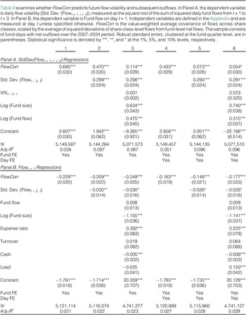
Since our measure of flow correlation is constructed from class-, not investor-level flows, it is important to verify that higher flow correlation is associated with greater flow volatility. To do so, we estimate regressions of subsequent flow volatility on FlowCorr. We measure flow volatility using the square root of the sum of squared daily flows over a 3-day window (using a t + 1 to t + 3 timing convention) and control for market volatility (VIX), fund size, and past flows. Robust standard errors are clustered at the fund-quarter level. Panel A of Table 2 reports these flow-volatility regressions for fund-days with net outflows. Column 1 presents a univariate regression with fund fixed effects (to absorb time-invariant fund heterogeneity), and column 4 additionally includes day fixed effects (to absorb common volatility spikes). In both specifications, future flow volatility is reliably positively related to FlowCorr. Since flow volatility is persistent, the regressions in columns 2 and 5 add lagged flow volatility as a predictor. As expected, the coefficient on lagged volatility is positive, but the coefficient on FlowCorr remains significantly positive. Lastly, columns 3 and 6 add measures of market volatility (VIX), fund size, and lagged flows. Each successive model is more stringent, and throughout the specifications, the coefficient on FlowCorr remains positive.

TABLE 2Flow Diversification, Future Flow Volatility, and Subsequent Flows

TABLE 2 Long description

The table presents regression results for fund-days with net outflows from 2007 to 2024.

Panel A: Dependent variable is daily flow volatility (Std. Dev. (Flow sub t plus 1, t plus 3)).

* FlowCorr: Coefficients range from 0.054 to 0.680, all statistically significant at the 1 percent or 10 percent levels.

* Std. Dev. (Flow sub t minus 2, t): Coefficients are approximately 0.29, significant at the 1 percent level.

* Log (Fund size) and Log (Fund flow): Both show positive significant coefficients around 0.63 to 0.74 and 0.31 to 0.47 respectively.

* Adjusted R-squared: Ranges from 0.038 to 0.096.

* Sample size (N): Approximately 5.1 million observations.

Panel B: Dependent variable is Fund flow on day t plus 1.

* FlowCorr: Coefficients are negative, ranging from minus 0.148 to minus 0.249, all significant at the 1 percent level.

* Std. Dev. (Flow sub t minus 2, t): Small negative coefficients around minus 0.03, significant at the 5 percent or 10 percent levels.

* Log (Fund size): Negative coefficients around minus 1.15, significant at the 1 percent level.

* Expense ratio: Positive significant coefficients.

* Adjusted R-squared: Ranges from 0.021 to 0.029.

Both panels include Fund Fixed Effects (F E) in all models, while models 4, 5, and 6 also include Day Fixed Effects (F E). Standard errors are clustered at the fund-quarter level and shown in parentheses below the coefficients.

Flow volatility is a reduced-form proxy for unexpected flows, but we can also assess whether flow correlation is related to unexpected flows directly. One could measure unexpected flows using a time series model, but the median autocorrelation in daily flows is only 0.03, implying that at the daily level, flows are largely unpredictable. To avoid overfitting a weakly persistent process, we use outflows in t + 1 as the dependent variable. Panel B of Table 2 reports the results for fund-days with net outflows. In the univariate specifications (with either fund or fund and day fixed effects), the coefficients on FlowCorr are −0.229 and − 0.163, showing that higher flow correlation, or lower flow diversification, is associated with larger next-day outflows. Adding lagged flow volatility in columns 2 and 5 attenuates the coefficients modestly, confirming the results in Rakowski (Reference Rakowski2010). In the full specifications that include controls for past flows (which further account for the modest serial correlation in daily flows described previously), fund size, expense ratios, turnover, cash levels, and loads, the coefficients on FlowCorr remain statistically significant at −0.249 and −0.177. These estimates imply that a 1-standard-deviation increase in FlowCorr is associated with larger next-day redemptions: the implied effects are 3.78% and 4.10% of the mean next-day outflow in the outflow-only sample, respectively.

Overall, the results in Table 2 establish that higher FlowCorr is related to both elevated future flow volatility and larger unexpected outflows, the mechanisms through which liquidity externalities arise. These findings validate the central premise of our identification strategy: flow correlation, even when measured through share-class flows rather than investor-level flows, captures economically significant differences in the synchronization of liquidity demands that are not captured by flow volatility alone.

A. Flow Diversification and Cash Buffers

If fund managers recognize that greater flow diversification lowers outflows, then, ceteris paribus, they should optimally hold less precautionary cash. The economic tradeoff underlying this prediction is between holding costly precautionary cash ex ante and incurring trading costs ex post when redemptions arrive. Holding cash creates cash drag, but this cost is relatively predictable and can be managed through the size of the buffer. In contrast, redemption-induced trading may require funds to sell securities quickly, generating explicit trading costs, bid–ask spread, and price impact that reduce fund NAVs. Thus, predictable flow correlation can be incorporated into cash-buffer decisions, whereas higher unexpected flow correlation is more likely to generate short-run trading pressure and lower post-outflow returns.

We test these predictions in two complementary ways. The first relates end-of-quarter cash buffers to average flow correlation over the quarter (ExpFlowCorr). Column 1 of Panel A in Table 3 reports a univariate regression with fund-year fixed effects, and column 3 augments this specification with fund and style-year fixed effects. The coefficients on ExpFlowCorr are 0.744 and 0.898, both of which are statistically significant. A 1-standard-deviation increase in ExpFlowCorr predicts a 2.78% and 3.35% increase in end-of-quarter cash buffers, respectively. In columns 2 and 4, we add controls for fund size, fund flows over the quarter, fund returns, daily flow volatility, expense ratios, loads, and turnover. The inclusion of these controls attenuates the coefficients on ExpFlowCorr, but they remain statistically significant.

TABLE 3Flow Diversification and Cash Holdings

TABLE 3 Long description

The table is divided into two main sections. Columns 1 through 4 represent Panel A, Regressions of End-of-Quarter Cash. Columns 5 through 10 represent Panel B, Regressions of Daily Changes in Cash.

In Panel A, the variable E x p Flow Corr shows positive coefficients across all models: 0.744 in column 1, 0.384 in column 2, 0.898 in column 3, and 0.476 in column 4. Standard errors are provided in parentheses below each coefficient.

In Panel B, the variables include:

* E x p Flow Corr: Coefficients are -0.083 in column 5 and -0.099 in column 6.

* Share class increase indicator: -0.123 in column 7 and -0.119 in column 8.

* Large share class increase indicator: -0.216 in column 9 and -0.217 in column 10.

* Small share class increase indicator: -0.038 in column 9 and -0.029 in column 10.

* Outflow indicator: 0.024 in column 5 and 0.021 in column 6.

* E x p Flow Corr times Outflow: 0.170 in column 5 and 0.158 in column 6.

Fixed Effects F E and Controls:

* Controls are included in columns 2, 4, 5, 6, 7, 8, 9, and 10.

* Fund-year F E is used in columns 1 and 2.

* Style-year F E and Fund F E are used in columns 3 and 4.

* Fund F E is used in all columns of Panel B (5 through 10).

* Day F E is used in columns 6, 8, and 10.

Summary statistics at the bottom show N values ranging from 130,736 in Panel A to over 8 million in Panel B. Adjusted R-squared values are high in Panel A (0.690 to 0.846) and lower in Panel B (approximately 0.02).

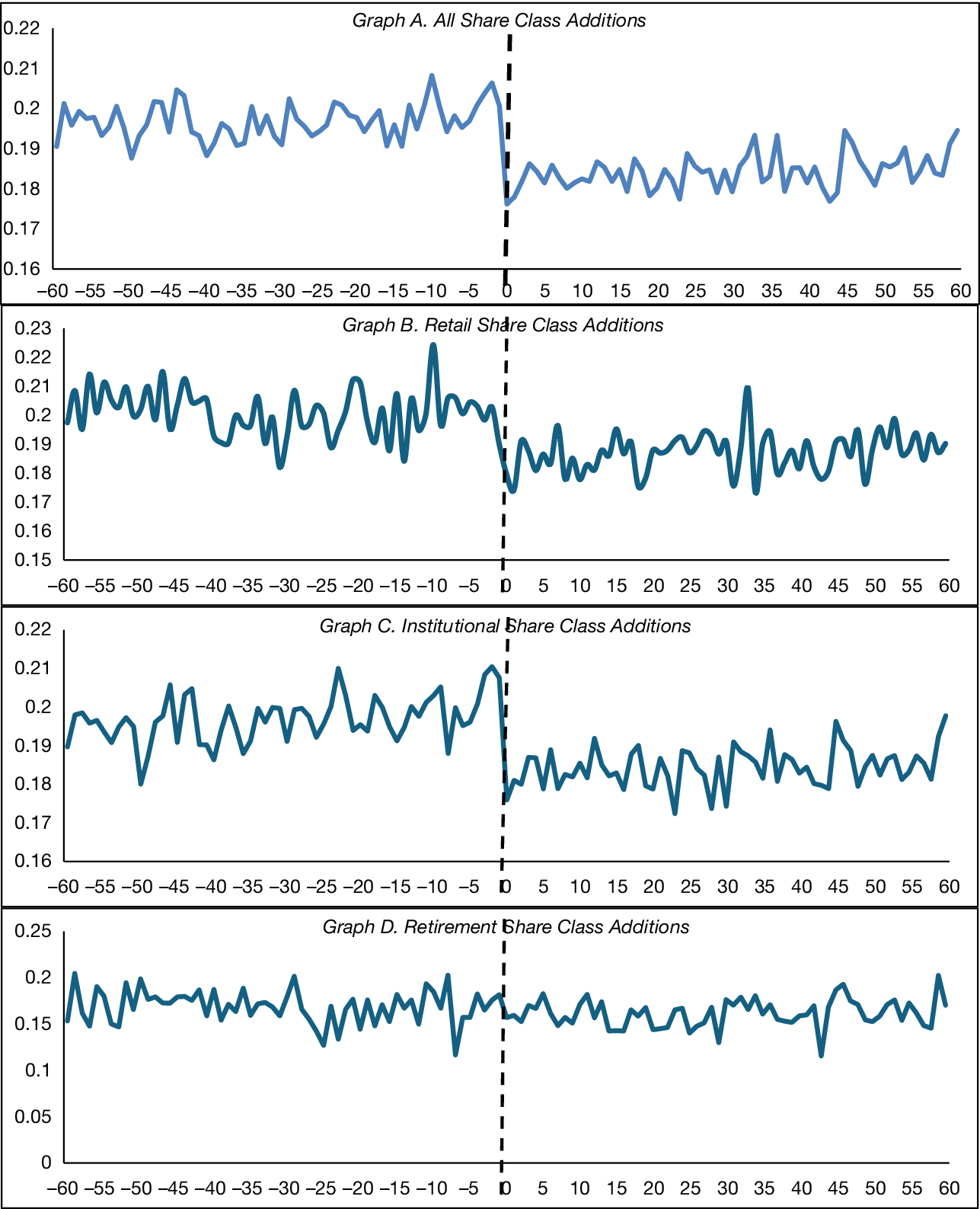
The second approach exploits changes in clientele composition by examining share-class additions, which should expand the investor base, reduce average flow correlation, and reduce cash buffers. Over our sample period, there are 6,552 share-class additions from a different clientele. Graph A of Figure 2 plots the cross-sectional average FlowCorr from 60 days before to 60 days after the addition of a share class. The graph shows a 6.39% decrease in flow correlation sharply centered around day 0. Graphs B through D repeat the analysis separately for retail, institutional, and retirement share classes. For retail and institutional additions, we continue to observe large declines in flow correlation around day 0. There is no significant decline around the addition of retirement share classes, likely reflecting the limited number of such events in our sample (only 258 events, compared to 1,834 retail class additions and 4,460 institutional share class additions).

FIGURE 2Change of Flow Correlation Around Share-Class Additions

Figure 2 presents an event-study analysis of flow correlation around share-class additions. Each graph shows average flow correlations from 60 trading days before to 60 trading days after the addition of a share class from a different clientele on day 0. Graph A presents results for all share class additions. Graphs B through D present results separately for retail, institutional/advisor, and retirement share class additions.

FIGURE 2 Long description

A multi-panel line graph with four vertical panels labeled A through D. All graphs share a common X-axis representing trading days from minus 60 to positive 60, with a vertical dashed line at day 0 marking the share-class addition.

* Graph A, All Share Class Additions. The Y-axis ranges from 0.16 to 0.22. Before day 0, the flow correlation fluctuates between 0.19 and 0.21. At day 0, there is a sharp vertical drop to approximately 0.175, followed by a lower-level fluctuation between 0.18 and 0.19.

* Graph B, Retail Share Class Additions. The Y-axis ranges from 0.15 to 0.23. The pre-event period shows high volatility between 0.18 and 0.22. After the drop at day 0, the correlation remains lower, mostly between 0.17 and 0.19.

* Graph C, Institutional Share Class Additions. The Y-axis ranges from 0.16 to 0.22. Similar to Graph A, it shows a stable pre-event range around 0.19 to 0.21 and a distinct drop at day 0 to a new range between 0.17 and 0.19.

* Graph D, Retirement Share Class Additions. The Y-axis ranges from 0 to 0.25. Unlike the other panels, the data is more compressed at the top of the scale. The flow correlation fluctuates around 0.15 both before and after day 0, showing a less pronounced drop compared to retail or institutional classes.

Panel B of Table 3 examines whether these declines in flow correlation translate into reductions in cash buffers. Cash holdings are reported at month- or quarter-end, but share-class additions are not subject to such discreteness. To manage these differing frequencies, we assume that daily cash equals the most recently reported value, updating it when new cash data becomes available. The dependent variable in our regressions is the change in cash buffers from day t − 20 to day t + 20.Footnote ¹¹ Because this sample includes both inflows and outflows, we first ask whether changes in cash buffers are symmetric for inflows and outflows. Columns 5 and 6 show regressions of change in cash on ExpFlowCorr, an indicator variable equal to 1 for outflows, and the interaction between the two variables. Column 5 uses fund fixed effects with standard errors based on Driscoll and Kraay (Reference Driscoll and Kraay1998), while column 6 uses fund and day fixed effects with standard errors clustered by fund and day.Footnote ¹² The interaction term is positive, implying that the relation between predictable flow correlation and changes in cash buffers is stronger for outflows than inflows.

Next, we examine the effect of changes in the number of share classes on changes in cash. Columns 7 and 8 regress this change in cash on an indicator variable equal to 1 if the number of share classes increases on day t with the same set of control variables as in Panel A. In both specifications (that use fund or fund and day fixed effects), share-class additions are associated with a reduction of roughly 3% in cash holdings.

The impact of adding a share class is likely nonlinear and depends on the pre-increase number of share classes. For example, an increase from two to three share classes is quite different from seven to eight. In columns 9 and 10, we replace the share-class increase indicator variable with separate indicators for large and small share-class indicators, in which “large” is defined as cases where the post-increase number of share classes is four or less. The coefficients on large additions remain negative and significant, implying a 5.3% decline in cash holdings. In contrast, the coefficients on small additions are indistinguishable from 0, suggesting that only economically meaningful expansions in clienteles drive reductions in precautionary cash buffers.

B. The Effects of Flow Diversification on Fund Performance

1. Univariate Sorts and Multivariate Evidence

We start our analysis of flow diversification and fund performance with sorts because they provide model-free and easy-to-interpret summary estimates. In Table 4, we sort all funds with outflows on day t into quintiles based on FlowCorr, UnexpFlowCorr, and ExpFlowCorr, and then compute benchmark-adjusted returns over subsequent horizons. Risk effects are unlikely to be important at short horizons, so factor model alphas are unnecessary. However, since liquidity differences associated with investment styles can be meaningful, we use benchmark-adjusted returns based on each fund’s equity style classification. Because flow diversification is measured on day t and trading externalities arise through short-horizon trading costs, we focus on benchmark-adjusted returns over days t + 1, t + 2, and t + 3 and the cumulative return from t + 1 to t + 3. Standard errors are computed from the time series of quintile returns with Newey–West adjustments to account for overlapping return windows.

TABLE 4Flow Diversification and Short-Horizon Fund Returns

TABLE 4 Long description

The table is divided into three panels, each containing columns for X R sub t plus 1, X R sub t plus 2, X R sub t plus 3, cumulative X R sub t plus 1 to t plus 3, cumulative X R sub t plus 1 to t plus 20, and Number of Funds.

Panel A: Benchmark-Adjusted Returns on Sorts of FlowCorr.

Quintile 1 (Low) has a t plus 1 return of minus 1.959 and a t plus 1 to t plus 20 return of minus 29.215.

Quintile 5 (High) has a t plus 1 return of minus 2.173 and a t plus 1 to t plus 20 return of minus 30.872.

The Low minus High difference is 0.214 for t plus 1 and 1.662 for t plus 1 to t plus 20, neither being statistically significant.

Panel B: Benchmark-Adjusted Returns on Sorts of UnexpFlowCorr.

Quintile 1 (Low) has a t plus 1 return of minus 1.796 and a t plus 1 to t plus 20 return of minus 28.345.

Quintile 5 (High) has a t plus 1 return of minus 2.247 and a t plus 1 to t plus 20 return of minus 32.654.

The Low minus High difference is statistically significant at 0.451 for t plus 1 (p < 0.05), 1.071 for t plus 1 to t plus 3 (p < 0.01), and 4.128 for t plus 1 to t plus 20 (p < 0.01).

Panel C: Benchmark-Adjusted Returns on Sorts of ExpFlowCorr.

Quintile 1 (Low) has a t plus 1 return of minus 2.077 and a t plus 1 to t plus 20 return of minus 31.400.

Quintile 5 (High) has a t plus 1 return of minus 1.996 and a t plus 1 to t plus 20 return of minus 29.389.

The Low minus High difference is minus 0.080 for t plus 1 and minus 1.461 for t plus 1 to t plus 20, showing no statistical significance.

Each quintile across all panels contains approximately 229 to 230 funds.

Panel A shows that funds in the lowest FlowCorr quintile earn higher subsequent returns than funds in the highest quintile, but the standard errors are large. For example, the 3-day spread in benchmark-adjusted returns between low and high FlowCorr quintiles is 0.55 basis points with a standard error of 0.35. The muted relation is unsurprising because the permanent component of FlowCorr is anticipated by fund managers and baked into cash buffers, reducing the need for immediate trading. Panel B shows quintiles based on UnexpFlowCorr and reveals a starkly different picture. Here we observe a strong, monotonic relation between unexpected flow correlation and subsequent returns; the 3-day benchmark-adjusted return spread between the lowest and highest UnexpFlowCorr quintiles is 1.07 basis points with a standard error of 0.30. By contrast, Panel C shows no meaningful difference in benchmark-adjusted returns across quintiles formed on ExpFlowCorr, consistent with the interpretation that fund managers understand predictable flow patterns from their share-class-based clientele and adjust cash buffers accordingly.

It is uncommon to measure trading-cost effects over longer horizons because cumulating returns over many days introduces substantial noise. Nonetheless, we examine returns over a 20-trading-day horizon for two reasons. First, a longer horizon allows us to verify that the return differences associated with flow diversification are not reversed, ensuring that the benefits accrue to longer term shareholders. Second, the 20-day horizon provides a useful bridge to the monthly return frequencies commonly used in the mutual fund literature. The last column in each panel in Table 4 shows results using 20-day benchmark-adjusted returns with 19 lags used in the Newey–West standard errors. In Panel A, the difference in returns between the low and high FlowCorr quintiles rises to 1.66 basis points but with a standard error of 1.43; the equivalent spread in returns for UnexpFlowCorr quintiles quadruples relative to the 3-day window, reaching 4.13 basis points with a standard error of 1.10. This indicates that the return differences associated with unexpected flow correlation are not transitory.

Table 5 complements the previous evidence with regressions of 3-day cumulative benchmark-adjusted returns (in basis points) on prior flow correlation measures. The regressions allow us to explicitly control for outflows on day t, as well as other covariates that may affect short-horizon fund returns. In addition to the usual controls, two variables are of particular importance. First, including cash buffers ensures that flow diversification is relevant beyond precautionary cash holdings. Second, lagged flow volatility isolates the influence of flow diversification from the broader flow volatility channel. Even with these control variables, a remaining concern is that unobservable fund-manager skill could be correlated with flow diversification, creating an omitted-variable bias. In column 1, we use fund fixed effects to absorb the variation in returns due to skill. Given our return measures are constructed over overlapping short-horizon windows, fund fixed effects also allow us to exploit within-fund variation over time without restricting identification to within-quarter changes. Column 2 adds day fixed effects to capture common liquidity or market-wide shocks on certain days.

TABLE 5Flow Diversification and Short-Horizon Fund Returns: Multivariate Regressions

TABLE 5 Long description

The table presents multivariate panel regressions for 3-day cumulative benchmark-adjusted returns.

Column 1 and 2 focus on FlowCorr:

- FlowCorr: -0.443 (0.128) in column 1 and -0.517 (0.121) in column 2, both significant at the 1% level.

Column 3 and 4 decompose FlowCorr into Expected and Unexpected components:

- ExpFlowCorr: 0.004 (0.600) in column 3 and -0.024 (0.577) in column 4, both statistically insignificant.

- UnexpFlowCorr: -0.480 (0.129) in column 3 and -0.557 (0.122) in column 4, both significant at the 1% level.

Control variables across all columns:

- Log (Fund size): Consistently negative around -1.9 to -2.0, significant at 1%.

- Log (Fund flow): Statistically insignificant across all models.

- Expense ratio: Significant at 1% in columns 1 and 3 (approx 2.0), but insignificant when Day F E is added.

- Turnover, Std. Dev. (Flow), and Cash: All statistically insignificant.

- Load: Significant at 1% in columns 1 and 3 (1.292), but insignificant in columns 2 and 4.

- Constant: Positive and significant at 1%, ranging from 29.296 to 33.713.

Model Specifications:

- Fund F E: Yes for all columns.

- Day F E: Yes for columns 2 and 4 only.

- N: Approximately 4.6 million observations per column.

- Adj-R squared: 0.003 for columns 1 and 3; 0.104 for columns 2 and 4.

Unlike the sorts, the multivariate regressions reveal a statistically significant negative relationship between FlowCorr and subsequent returns. In columns 1 and 2, the coefficients on FlowCorr are −0.44 and −0.52 with standard errors of 0.13 and 0.12; a 1-standard-deviation decrease in FlowCorr is associated with a 3.88% and a 4.53% increase in the average 3-day benchmark-adjusted return, respectively. Columns 3 and 4 replace FlowCorr with its decomposed counterparts. Consistent with the portfolio sorting results in Table 4, the coefficients on UnexpFlowCorr are negative and statistically significant, while the coefficient on ExpFlowCorr is indistinguishable from 0. A 1-standard-deviation decrease in UnexpFlowCorr implies a 3% improvement in the 3-day benchmark-adjusted return (0.22 basis points). Table 6 extends the analysis to 20-day benchmark-adjusted returns (in percentage), allowing us to assess whether the trading-cost effects associated with flow diversification persist rather than reverse. The coefficients on FlowCorr remain negative and statistically significant. Moreover, decomposing FlowCorr again reveals that the predictive power resides in UnexpFlowCorr: the coefficient on ExpFlowCorr remains statistically indistinguishable from 0, while the coefficient on UnexpFlowCorr continues to be negative and statistically significant. Quantitatively, a 1-standard-deviation decrease in UnexpFlowCorr implies a 1.5% increase in the 20-day benchmark-adjusted return (0.47 basis points).

TABLE 6Flow Diversification and 20-Day Benchmark-Adjusted Fund Returns

TABLE 6 Long description

The table presents panel regression results for 20-day cumulative benchmark-adjusted returns.

Column headers are numbered 1 through 4.

Independent variables and their coefficients (standard errors in parentheses):

* FlowCorr: -0.010** (0.004) in columns 1 and 2.

* ExpFlowCorr: 0.010 (0.036) in column 3 and 0.017 (0.035) in column 4.

* UnexpFlowCorr: -0.012*** (0.004) in column 3 and -0.012*** (0.003) in column 4.

* Log (Fund size): -0.151*** (0.008) across all four columns.

* Log (Fund flow): 0.010*** (0.001) in columns 1 and 3; 0.003*** (0.001) in column 2; 0.003** (0.001) in column 4.

* Expense ratio: 0.082* (0.046) in columns 1 and 3; 0.042 (0.051) in column 2; 0.041 (0.050) in column 4.

* Turnover: 0.002 (0.002) across all four columns.

* Std. Dev. (Flow sub t minus 2, t): 0.000*** (0.000) in columns 1 and 3; -0.000*** (0.000) in columns 2 and 4.

* Cash: -0.002 (0.002) across all four columns.

* Load: 0.086*** (0.019) in columns 1 and 3; -0.019 (0.020) in columns 2 and 4.

* Constant: Values range from 2.527*** to 2.656***.

Fixed Effects and Statistics:

* Fund F E: Yes for all columns.

* Day F E: Yes for columns 2 and 4; blank for 1 and 3.

* N: 4,329,763 for columns 1 and 3; 4,329,747 for columns 2 and 4.

* Adj-R super 2: 0.022 for columns 1 and 3; 0.115 for columns 2 and 4.

Statistical significance is denoted by *** at 1 percent, ** at 5 percent, and * at 10 percent levels.

Taken together, the return evidence in this section and the cash-holding results in Section V.A support the interpretation that predictable differences in flow correlation are partly absorbed through managerial liquidity management, while unexpected increases in flow correlation are associated with lower post-outflow returns.

C. Alternative Mechanisms

Several mechanisms can mitigate redemption-induced trading. Swing pricing shifts trading costs from remaining investors to redeeming shareholders (Jin, Kacperczyk, Kahraman, and Suntheim (Reference Jin, Kacperczyk, Kahraman and Suntheim2022)), although none of the U.S. equity funds in our sample employ swing pricing based on N-CEN filings from 2019 to 2024. Redemption-in-kind allows funds to meet redemptions by transferring securities rather than selling them, but actual usage is rare: Agarwal, Ren, Shen, and Zhao (Reference Agarwal, Ren, Shen and Zhao2023) document only 2,985 redemptions-in-kind across 58,443 fund-years. Asset managers have also converted mutual funds into ETFs, which use in-kind redemption processes to reduce trading and tax externalities under Rule 6c-11 (Du, Starks, and Xiaolan (Reference Du, Starks and Xiaolan2023)). Relatedly, the expiration of Vanguard’s patent on ETFs as a share class in 2023 has prompted some asset managers to seek regulatory approval to include ETFs as a share class within a mutual fund.Footnote ¹⁵ These mechanisms share a common objective: shifting trading activity away from the fund.

Our results indicate that flow diversification itself operates as a natural buffer. While redemptions create immediacy demands that can depress fund returns, greater heterogeneity in investor liquidity needs reduces the likelihood that redemptions arrive simultaneously. This mitigating effect is particularly important in settings where shareholders anticipate the redemptions of others, since such expectations can generate multiplier effects or shareholder runs, contributing to fragility in financial markets. We turn to this next.

D. Multiplier Effects

Chen, Goldstein, and Jiang (Reference Chen, Goldstein and Jiang2010) argue that investors in illiquid funds face a higher degree of strategic complementarity because redemptions from illiquid assets impose larger trading costs on remaining shareholders. Exploiting this insight, their test of strategic complementarity consists of regressions of flows on prior performance in which the key explanatory variable is the interaction between an illiquidity indicator and prior performance.

If a fund has diversified flows, then shareholders may be less concerned with the exit of other investors, weakening strategic complementarities. This intuition translates into two tests. First, we aim to determine whether funds with higher flow diversification have lower flow-performance sensitivity, notwithstanding the higher flow-performance sensitivity of illiquid funds. Second, we ask whether flow-performance sensitivities in illiquid funds vary with flow diversification; in other words, can flow diversification at least partially offset strategic complementarities, even when they exist? To implement these tests, we make two modifications to the Chen, Goldstein, and Jiang (Reference Chen, Goldstein and Jiang2010) approach. First, because we use higher frequency daily flow data to measure liquidity effects, we measure performance over the prior 3 days rather than using alphas from a factor model.Footnote ¹⁶ Second, we estimate regressions at the fund rather than the share-class level to align our fund-level flow correlation measure built from share-class flows. Aside from these changes, the regressions closely mirror Table 2 and contain the same set of control variables. Our key additions are i) an indicator variable FlowCorr(I), equal to 1 for funds with higher flow correlation (above median) or lower flow diversification; ii) interaction terms between FlowCorr(I) and prior performance; and iii) triple interaction terms between FlowCorr(I), prior performance, and the illiquidity indicator. We estimate these regressions separately for the fund-days with inflows versus outflows because strategic complementarities should be most relevant for outflows.

Panels A and B of Table 7 report results for outflows and inflows, respectively. The dependent variable is winsorized proportional fund flows (at the 1st and 99th percentiles). The first two columns in each panel include fund fixed effects, while the last two columns add day fixed effects to absorb common shocks in the time series. Across all specifications, the interaction term between the illiquidity indicator and prior performance is positive and statistically significant, replicating the results in Chen, Goldstein, and Jiang (Reference Chen, Goldstein and Jiang2010). Using monthly data, their estimates imply that flow-performance sensitivity is 52% higher in illiquid funds; by comparison, in column 3 with fund and day fixed effects, the equivalent increase in flow-performance sensitivity is 49.4% (0.166/(0.170 + 0.166)), remarkably similar in magnitude.

TABLE 7Daily Flow-Performance Regressions

TABLE 7 Long description

The table consists of 8 columns of regression results. Columns 1 through 4 represent Panel A (Prior 3-Day Outflows) and columns 5 through 8 represent Panel B (Prior 3-Day Inflows).

Key variables and coefficients (standard errors in parentheses):

* Perf.: Values range from 0.170 to 0.392 in Panel A and 0.367 to 0.394 in Panel B. All are significant at the 1% level.

* Illiq. indicator: Coefficients are small (0.007 to -0.001) and mostly insignificant.

* Perf. * Illiq. indicator: Positive and significant across all models, ranging from 0.054 to 0.166.

* FlowCorr (I): Positive and significant at the 1% level across all models, ranging from 0.008 to 0.014.

* Perf. * FlowCorr (I): Significant in Panel B (0.265 to 0.307) but mixed in Panel A (0.029 to 0.098).

* Illiq. Indicator * FlowCorr (I) * Perf.: Significant positive interaction in Panel A (0.100 to 0.116) but negative and insignificant in Panel B (-0.056 to -0.064).

Model Statistics:

* Controls: Yes for all models.

* Fund F E: Yes for models 1, 2, 5, and 6.

* Fund F E and Day F E: Yes for models 3, 4, 7, and 8.

* N (Observations): Approximately 5.06 million for Panel A and 3.21 million for Panel B.

* Adj-R squared: Ranges from 0.025 to 0.036 in Panel A and 0.072 to 0.080 in Panel B.

Columns 1 and 3 show that the interactions between FlowCorr(I) and prior performance are positive and significant, indicating that flow-performance sensitivity is higher in funds with larger flow correlation. In column 3, which includes fund and day fixed effects, the magnitude of this difference is economically meaningful: dividing the coefficient on the interaction between FlowCorr(I) and Perf. by the coefficient on Perf. alone implies that flow-performance sensitivity is 49% (0.084/0.170) higher for funds with lower flow diversification. Panel B shows a similar positive interaction for inflows, suggesting that less diversified clienteles may be more performance-sensitive. These results show that even in the presence of strategic complementarities, flow diversification continues to play an important mitigating role.

We next turn to the specifications most relevant for our mechanism, which include the triple interaction terms between FlowCorr(I), prior performance, and the illiquidity indicator. The goal is to ask whether flow-performance sensitivities in illiquid funds vary with flow diversification. Across all columns in Panel A, the coefficients on the triple interaction are significantly positive, indicating that illiquid funds with low flow diversification exhibit the strongest strategic complementarities. In column 4, which includes fund and day fixed effects, the flow-performance sensitivity of illiquid funds with high flow diversification is 0.200 + 0.113 = 0.313. For low flow-diversification funds, the coefficient on the triple interaction is 0.100, implying that the increase in flow-performance sensitivity is almost 31% higher (0.100/0.313). In contrast, in Panel B, the triple interaction effect is indistinguishable from 0. Taken together, these results indicate that while low flow diversification is associated with greater performance sensitivity more generally, the amplification of strategic complementarities in illiquid funds is concentrated in outflows, where redemption externalities are most relevant.

E. Alternative Measures of Flow Diversification

As robustness checks, we consider two alternative approaches that vary either by the weighting scheme or the underlying construction of flow diversification. The first alternative replaces value weights with equal weights while using proportional (instead of dollar) flows. Panel A of Table A4 shows that performance regressions using this measure generate very similar inferences. The second alternative measure focuses on flow imbalance, summing signed dollar flows across the K share classes and scaling by the sum of their absolute values. The measure is analogous to order imbalance in the market microstructure literature and resides in the interval (−1,+1). Since the numerator is signed, the measure is negative when a fund has outflows, and as a result, higher flow imbalance in absolute value (distance from 0) indicates less offsetting flow across share classes and hence lower flow diversification. Because our focus is on outflows, we use the absolute value of flow imbalance in our tests (|FlowImb|). The regression results in Panel B of Table A4 also show a negative coefficient on the unexpected component of |FlowImb|, but the coefficient on the expected component is indistinguishable from 0.