GRAIN PRICES AND GRAIN TRADE IN INDIA

Before looking into this issue, we first need to become acquainted with the sources of evidence and the background to the question.

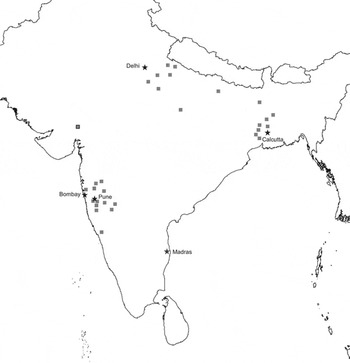
For the intended investigation, grain price quotations for India, which encompass the period from 1700 to 1914, have been collected from a variety of sources, including government papers, old statistics journals, and the secondary literature. The early series are normally based on information from civil or military authorities (both Indian and English), Indian revenue functionaries (mamlutdars), or wholesale traders. Only the two most widely recorded grains—wheat and rice—were included, and the price series represent annual average prices, either for calendar years or for harvest years (June–May).Footnote ⁷ In total, 54 price series for 35 different cities could be compiled for the prestatistical era, of which ten cities or market places are located in eastern India, 16 in western India, eight in northern India, and only one in Madras in the south (see Figure 1).

Figure 1

LOCATION OF MARKETS WITH PRE-1860 PRICE SERIES

Sources: See the text and the Appendix.

For reasons of temporal comparison, some additional markets for the period after 1860 (for which an abundance of price data are available) have been included in the study, so that the final database for the present investigation consists of 70 different price series (36 for wheat and 34 for rice) for 46 cities, which are spread all over the subcontinent. In many senses, this dataset is quite limited, and heterogeneous too, not only because of the wide variety of sources it draws upon. The markets, for which data were available, vary greatly in their economic importance—from local to metropolitan—as do the time periods that the various price series cover. The average number of years a price series covers continuously is 47; the minimum number and maximum numbers being 19 and 160, respectively. And whereas a majority of the series were recorded under British rule, many were not, and several price series even pre-date British arrival in that particular part of the country by half a century or more.Footnote ⁸

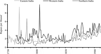
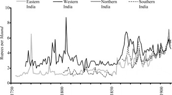
To further acquaint the reader with the data, Figure 2 presents wheat price series for the different major regions in India between 1750 and 1914. These long price series already reveal some general features of the grain prices in eighteenth- and nineteenth-century India. First and foremost, Figure 2 reveals that the comparative price pattern before the 1850s looks fundamentally different from the post-1850 pattern.

Figure 2

CONVERGENCE OF WHEAT PRICES

Sources: See the text and the Appendix.

In the pre-1850 period, the price levels in all regions remained fairly stable, but there were shorter periods of rising or falling prices that can be observed. Although prices fluctuated massively from year to year in all parts of India, prices were higher in the west than in Bengal or in the north. Before 1850 these year-to-year price movements seem completely unrelated in regions that were distant from one another; even the massive price spikes did not coincide. The enormous price inflations are also an impressive testimony of the severe harvest failures that led to the Bengal famine of 1770 and to famines in the north (1783) and the west (1804) of the country. The fact that the price increases during these crises was far higher than the ones during the terrible famines of 1876/77 and 1896/97 bode ill for the social and demographic impacts of the earlier famines, about which little is known.

In the post-1850 period, prices rose permanently in all regions until the outbreak of the World War. Not only did prices inflate similarly in all three regions during this later period, but the short-term variations also looked very similar. This feature contrasts starkly with the totally asynchronous price movements observed for the early period.

Before we use this price database to assess the efficiency of Indian grain markets, let us first briefly describe how grain was produced and transported.

The spatial and temporal growing patterns of rice and wheat—as with all Indian agricultural products—were (and to some extent still are) above all determined by the monsoon, in particular the southwest monsoon (June–September), which supplies India with most of its annual rainfall. Rice, as a crop with a high water requirement, was the dominant crop in regions with high annual rainfall, such as Bengal, the eastern Indo-Gangetic plains, the coast of Konkan, Malabar, Tamil Nadu, and the Krishna-Godavari delta. It was grown in the summer or “kharif” growing season, which coincides with the southwest monsoon. Wheat, with a considerably lower water requirement (a “rabi” or dry-season crop) was planted in the postmonsoon season (October–November) and harvested in February–March.Footnote ⁹ The most important wheat growing regions were the Punjab and the western Indo-Gangetic plains.

But in prerailway India, the monsoon not only shaped production of food grains but also their transport. Because the heavy rainfall rendered road, river, and sea transport virtually impossible, most trade was carried out in the dry winter months from November to April.Footnote ¹⁰

Historians contend that grain, as other goods, was traded on three different levels in pre-British India: local, regional, and long-distance, and much of that trade was in the hands of special merchant communities such as the Vanjari or the Banjara. Of the food grains traded, rice and wheat were certainly the most important.Footnote ¹¹ Whereas the qualitative picture—what was traded, by whom, and when—is well known, the quantitative aspect—how much grain (and other goods) was traded on the different levels and how efficient the markets for various products were on the subcontinent—is largely unknown, and is an issue of debate due to the shortage of economic data for the period preceding the British takeover in 1858.Footnote ¹²

In the absence of widespread statistics on the volume of trade or on transport costs and transport capacities, the efficiency and extent of grain trade can only be gauged using price data. The comparative analysis of grain prices from different markets has proved to be a valuable and reliable means for inferences about the extent of trade, the efficiency of markets, and the processes of integrating or disintegrating markets, and it has been applied for many countries in numerous studies.Footnote ¹³ This makes sense as prices of widely consumed and traded goods—and grain was the most important in all pre-industrial economies—show several characteristics in integrated markets that they do not in fragmented markets, while the processes of increased (decreased) integration also exhibit characteristic price patterns. As a result, there are various formal methods for using grain prices to determine both the extent of market integration and the processes by which markets integrate, and we begin with the former.

GAUGING THE EXTENT OF GRAIN MARKET INTEGRATION

When market areas expand and formerly separated market places become part of one single market, the way prices are determined in these markets fundamentally changes. In totally unconnected markets, the local price of a product is determined by its local demand and supply. In the case of grain, it is the supply side—the annual harvest—which is by far the most important factor affecting prices in pre-industrial societies. Demand, by contrast, was very stable in the short term, as grain dominated the diet of the people and it was difficult to find substitutes. It modern terms, grain was a good with a low price elasticity. At the other extreme, when markets are perfectly integrated, the domestic price is independent of the local harvest: if the domestic market is small relative to the rest of the “world,” local harvest fluctuations only change the volume of imports or exports, while the domestic price equals the world price plus transport costs. (Here the “world” should not be taken literally; it simply stands for the geographical extension of the single market, of which the domestic market constitutes a small part.)

Over the last centuries, most places on earth have witnessed a dramatic change from a situation of nearly complete isolation to a state of close integration into a global market. This secular trend has not been without setbacks, and it has varied greatly for different products. Grain markets, with which this article is concerned, became integrated considerably later than markets for many other products. This is because grain has a very high bulk-to-value ratio, and therefore requires a much more effective transport infrastructure than goods with a low bulk-to-value ratio such as fine cloth or spices.

Turning to India, we will be looking at such a transition towards more integrated grain markets in the eighteenth and nineteenth centuries. As a result, we will often be confronted with “partial integration” of two markets, meaning that the domestic price of grain is influenced by the local harvest and the world grain price. Hence it is appropriate to gauge both the importance of the local harvest and of the world price on the domestic price.Footnote ¹⁴ However, because only price data and no harvest data are available, it is only possible to gauge to what extent the domestic price is connected to the world price; that is to say, how much the actual situation resembles the polar case of perfect integration. In perfectly integrated markets, it is the “law of one price” that determines the domestic price. The underlying logic of this so-called law is that once trade participants in two markets share the same information and transport costs become small, price differentials between markets offer opportunities for arbitrage up to the point that prices are either the same in the two markets or reach a stable ratio where the difference in price equals transport costs. As a consequence, the two price series are expected in the long-run to show a linear relationship, while small local price shocks, which temporarily create disequilibria in this stable relationship, are quickly corrected for by arbitrage. Testing whether the newly compiled grain prices show these two characteristics therefore serves as the basic means for gauging the extent of grain market integration in India before 1914.

We begin by scrutinizing the first characteristic of prices in integrated markets—whether they show a stable linear long-term relationship. The tool that is often applied to test for the presence of a linear relationship between stationary data series is correlation analysis.Footnote ¹⁵ Correlation analysis treats any (two) variables symmetrically, so that a single number, the correlation coefficient, describes the association between these variables.Footnote ¹⁶ The higher the coefficient, the stronger is the association between the variables. Hence higher coefficients suggest a more integrated market, and they are expected to decrease with the distance between two markets as transport costs rise.

This interpretation of correlation coefficients is, however, not without problems. High correlations of price series from two markets might also result from sources other than an integrated market. The most likely other source of high correlation is similar weather conditions in the two places, which would—also assuming similar production methods—lead to similar variations in yields. Consequently, as prices in fragmented markets are largely determined by local harvests—which, in turn, are heavily dependent on local weather—one would expect similar price movements in two markets, even though they might be totally unconnected. As we will see, the correlation coefficients derived from the Indian data make such an explanation highly unlikely. The problem of spurious correlation would be amplified if one were to use monthly data instead of annual data, for then part of the correlation could reflect seasonal price patterns that were very similar over large geographical areas, irrespective of how closely markets were linked.Footnote ¹⁷

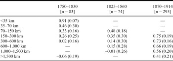
The results of the correlation analysis are presented in Table 1, and they have been grouped into three different time periods and according to the distance between markets. For the period from 1750 to 1830, 25 markets could be analyzed, while prices from only 15 cities were available for the years 1825–1860. In the later years from 1870 up to World War I, even though there is an abundance of data, the analysis was restricted to 20 different markets.Footnote ¹⁸ Combining the price series of these cities with each other, 450 binary relations (correlations) were examined in total, of which 83 are for the first period under consideration, 74 for the second, and 293 for the third. For various reasons, the number of binary relations actually analyzed is—in particular for the pre-1860 periods—far below the number one would expect given how many markets there are in the sample. The reason is that missing data make it impossible to calculate all the correlation coefficients. For instance, for the years 1750—1830, none of the price series covers the entire period, and many series do not overlap enough to estimate correlation coefficients reliably.Footnote ¹⁹ Also, for some markets only wheat or rice prices are available, but the correlations all involve prices for the same grain in different markets and so cannot be calculated if we have only a wheat price in one market and only a rice price in another. The same problem arises if there are differences in the way annual averages were computed, for it was harvest years in some cases and calendar years in others. Moreover, only “sensible“ relationships were included, meaning that very unlikely connections (such as between a tiny market in the western hinterlands and an eastern trading center) were dropped for the early period, which might bias the coefficients upwards compared to other studies.

Table 1

PRICE CORRELATIONS IN INDIA

Notes:

n = the total number of market pairs examined. Standard deviations are in parenthesis. Distance ranges with n ≤ 3 are not reported. The correlations concern pairs of wheat prices or pairs of rice prices; all prices are annual averages.

Sources:

See the text and the Appendix.

The results of the correlation analysis reveal above all a story of fundamental change. For the second half of the eighteenth century and the beginning of the nineteenth century, the law of one price is confirmed only in a local context; neighboring villages or cities less than 35 km apart clearly exhibit a common price regime. But already the mean coefficient for the next distance range, spanning from 35 to 70km, is drastically lower (0.46), while the variation between the coefficients (summarized by the standard deviation) shoots up compared with the local level (0.30 compared to 0.07). This suggests that the prices of some market pairs in this distance range were still closely connected, while for others, such a connection was already very weak. The connection of prices becomes very weak for markets that are 70 to 300km apart from each other, while for prices in cities that are separated by more than 300km, no mutual influence is discernible.

Only a cautious interpretation can be attempted about how this situation of highly fragmented and localized markets changed over the next decades (1825–1860). Because prices from fewer cities were available for this period, and none were located closer than 100km of each other, the local and regional situation escapes our view. Judging from the slightly increased coefficients at all distance levels for which data are available for both periods, one might draw the conclusion that there was some, albeit very limited, progress.

The pace of market integration, however, increased dramatically in the period of the railway construction after 1860. The coefficients for the years from 1870 to 1914 increased for all distances to such an extent that one could now talk about a national market in which the prices in two cities, no matter how far apart, rose and fell together. Over a century, progress was so far-reaching that prices in places 1,000–1,500km apart were now more closely tied than in cities 35–70km apart 100 years before.

But what do these correlations say about the Great Divergence debate? For this purpose, a database of wheat and spelt prices has been collected for Europe, which—in order to assure a maximum degree of comparability—shares some of the features of the Indian database. It consists of 20 markets, which (as in India) vary greatly in their economic importance. The markets are once again spread over the whole continent and yield information for all distance ranges. Most are not located on the coastline but are (as in the Indian case) landlocked. Prices are also annual rather than monthly, even though the latter type of data are widely available for Europe and have often been favored for studies on European market integration. Finally, as with the Indian evidence, the dataset covers the period 1700–1914. However, as sources on grain prices for Europe are much more abundant than in the Indian case, the coverage is much more complete, so that the average number of years encompassed by a price series is now 170 years; the maximum and minimum number are 205 and 45.Footnote ²⁰

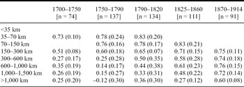
As a result, the correlation analysis could be extended back to 1700 for Europe, and the first examination period used in the analysis for India (1760–1830) could be subdivided into two separate periods. The later examination periods, 1825–1860 and 1870–1914, are the same. Over the whole period 1700–1914, 547 binary relations (correlations) were examined in total, and the numbers of market pairs examined in each subperiod are again shown in square brackets.

Although the presentation of the correlation results for Europe in Table 2 is identical to the one for India in Table 1, the results themselves are strikingly different.Footnote ²¹ In the first half of the eighteenth century, regional markets in Europe were already closely connected with a correlation coefficient of 0.73 for a distance range of 35–70km. Prices in markets up to 300km apart also show a considerable co-movement. Yet long-distance trade in grain must still have been very limited, as the connection between prices becomes very weak for all markets that were more than 300km apart. This picture of fragmented long-distance markets does not alter over the next decades. Regional and intraregional markets, however, become more and more integrated; for the period 1750–1790 prices in markets up to a distance of 300km were clearly heavily influenced by the same market forces. At around the turn of the nineteenth century, the geographical expansion of markets started to extend to the long-distance trade; in the 1790–1820 period the correlation coefficient is 0.5 or higher for markets up to a range of 600km.

Table 2

PRICE CORRELATIONS IN EUROPE

Notes:

Notes: n = the total number of market pairs examined. Standard deviations are in parenthesis. Distance ranges with n ≤ 3 are not reported. The correlations concern pairs of wheat prices or pairs of rice prices; all prices are annual averages.

Sources:

See the text and the Appendix.

The difference to India is striking: There, correlation coefficients of 0.5 or higher were restricted to local markets closer than 35km during the first examination period (1760–1830). Meanwhile, in Europe many markets even up to distance of 1,000km were now (1790–1820) reasonably connected, as can be deducted from the large standard deviation (0.38) for the distance range of 600–1,000km. Complete integration of grain markets did require decades more of steady market expansion, driven by the emergence of modern transport and information systems and by less protective trade policies. Yet by the late nineteenth century a truly all-European grain market did seem to exist, as is clear from the consistently high correlations coefficients and low standard deviations for all distance ranges in the years 1870–1914. If these numbers for the last period are compared with the results for the earliest period, it becomes apparent how far-reaching the changes in the eighteenth and nineteenth centuries were for economic integration: correlation coefficients that had once been typical of regional markets only 35–70km apart were by the late nineteenth century commonplace in markets 1,000–1,500km from one another. This was a truly revolutionary development.

The comparative picture emerging from Tables 1 and 2 is one of similar trends but stark differences in the timing and level of market integration. In both Europe and India, the extent of trade and the degree of market integration in 1900 were radically different from what they had been in 1700 or 1750. By the turn of the twentieth century both regions had grain markets that spanned their entire continent or subcontinent respectively and both were closely integrated into the world markets for grain.

Yet the level of market integration was always higher in Europe. This gap did vary greatly over time. Europe started at a considerably higher level of market integration than India; the correlation results suggest that Europe's level at the beginning of the eighteenth century already surpassed what India would attain in the late eighteenth and early nineteenth centuries. By then the extent of trade and the efficiency of markets were radically different in the two regions, and the striking differences persisted through the first half of the nineteenth century. In India, economic integration did not really start until the second half of the nineteenth century; it then proceeded at a very fast pace, making the period one of rapid catch-up for India. Nevertheless, the improvements were not quite far-reaching enough to close the gap; market efficiency as measured by correlation coefficients was even higher in Europe.

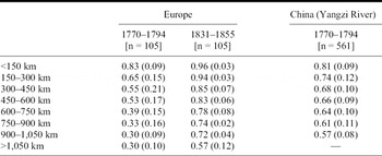
How then do the results for Europe and India compare with existing studies of market integration? One of the most extensive such studies, by Carol Shiue and Wolfgang Keller, compares Europe and China in the eighteenth century. Their results are reproduced in Table 3, which is based on a sample of monthly grain prices for 34 Chinese and 15 European markets.Footnote ²²

Table 3

PRICE CORRELATIONS IN CHINA AND EUROPE

Notes:

n = total number of market pairs examined. Standard deviations are in parentheses.

Sources:

Shiue and Keller, “Markets in China and Europe,” NBER paper 2004, tables 2a and 2b. Their prices are normally rice prices for China and wheat prices for Europe. Also, there are varying datasets for both China and Europe. However, the results using different datasets are broadly comparable. Most of their prices are monthly prices, but some are annual prices.

Clearly, Shiue and Keller trace a trend for Europe that is similar to the one shown in Table 2. Yet their coefficients are systematically larger, suggesting a higher level of market integration than the one proposed by Table 2. The main factor is no doubt the very different sample of markets used. Whereas the large majority of cities used in the present study are located in landlocked parts of Europe, Shiue and Keller's data are mostly for places with either direct or nearby access to the sea.Footnote ²³ Because water transport was far cheaper and faster than overland transport in the prerailroad era, it is hardly surprising that Shiue and Keller find a higher degree of market integration for their sample.Footnote ²⁴

The implication seems to be that European market integration has sometimes been overestimated. Landlocked Europe, which lacked Britain's or the Low Countries' endowment of natural waterways, did have well integrated grain markets on a regional and interregional scale of up to, say, 300km. Yet the present evidence does not corroborate popular views on long-distance trade, such as Karl Gunnar Persson's claim of an “emerging integrated European wheat market” in eighteenth-century Europe.Footnote ²⁵ The expansion of commerce that included the widespread long-distance trade in bulky goods and led to the formation of a European grain market had to await the nineteenth century. Such a conclusion does, of course, underline the importance of the railways for Europe's economic integration.

If we look at Shiue and Keller's results for the Yangtze River, the coefficients are actually slightly higher than for Europe, suggesting that markets in that part of China were at least as integrated as they were in Western Europe, and much more integrated than on the Indian subcontinent. Yet some caution is necessary here, because the Chinese sample—from the area drained by the Yangtze River—is by definition biased towards markets with cheap river transport.Footnote ²⁶

AN ERROR CORRECTION APPROACH

While correlation analysis can detect linear relationships between prices, error correction (EC) enables us to do more and test not just for the co-movement of prices but also for adjustment processes between markets. The basic idea underlying this method is that if price series in two markets show a linear relationship, then short-term shocks cannot disturb the relationship permanently because arbitrage will eventually restore it. The higher the efficiency of the markets—that is, the more integrated the markets are—the faster the equilibrium price ratio will be re-established.

A simple version of such an “error-correction model” (ECM) relates changes in the price in one city to an equilibrium error term, which is defined as the extent to which the stable price ratio between the city and a second market happened to deviate from equilibrium in the preceding time period. The more two markets are integrated, the faster the stable relationship will be re-established, and the bigger the coefficient of the price error correction term will become. Accordingly, the degree of co-movement of the price series will rise with the level of market integration.

Because little information about transport costs and markets structures is available, only a very simple model can be estimated;

(1)

(2)

and θ ₂ are the error correction coefficients, which indicate how fast each market adjusts to shocks. The degree of co-movement of the prices in P ₁ and P ₂ is measured by the correlation, ρ, between the error terms ε _{1, t} and ε _{2, t}, which are assumed to be normally distributed with mean zero. Finally, the constants c ₁ and c ₂ capture the long-run differences in the price levels, and they have been left unrestricted to allow for different transport cost in either direction. As a result, all the parameters in equations 1 and 2 are unrelated, and the equations can thus be estimated by simple OLS regressions. To eliminate problems arising from nonstationarity, the series used were differences in the logs of prices and gaps between the logs of prices.

The model here is made bivariate to allow for adjustments in both markets. Not doing so would imply that one of the prices is exogenous, that is to say that only one market responds to price disequilibria. In other words, one would impose an assumption that one of the two markets is always dominating, and such an assumption can simply not be justified given the scant information about the market structures in earlier periods. Because the terms (logP ₁ – logP ₂)_{t– 1} and (logP ₂ – logP ₁)_{t– 1} are the price gaps at time t – 1, θ ₁ and θ ₂ therefore measure the fraction of the price differential at t – 1 that is corrected for in one period t. In functioning markets, we expect θ ₁ < 0 and θ ₂ > 0, and we interpret higher absolute values of these coefficients as a sign of more efficient markets.

Because we are primarily interested in the speed of the adjustment and less so in the market structure between two cities, we also estimate the so-called marginal version of the model above. This enables us to estimate the total adjustment, γ, which combines the adjustment process in both markets, together with the significance level of the total adjustment. To derive the marginal model, we subtract equation 2 from 1

By substituting

we get

(3)

The total adjustment γ does not depend on which market of a market pair we label P ₁ and P _2, and we expect γ < 0 in functioning markets. The bigger the value of γ, the faster the overall adjustment process. Hence a larger γ points to more efficient markets. We also want to test the hypothesis of whether the total adjustment, γ, really is significant, which is to say that we test whether γ = 0. Because the appropriate test statistic for this is Dickey-Fuller distributed rather than standard normal, the critical value at a 95 percent confidence level (one-sided test) is –2.86 instead of –1.64.Footnote ²⁷ Again, equation 3 can be estimated by OLS regression.

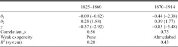
To see how this error correction model works and how the results are interpreted, let us consider an example, from the cities of Pune and Ahmedabad, both located in western India some 660km apart. Using annual rice prices from the two cities, we first estimate the system given by equations 1 and 2, and then the marginal model given by equation 3. From equations 1 and 2, we get estimates for θ ₁ and θ ₂, for ρ (the correlation between the error terms ε _{1, t} and ε _{2, t}), and for R ². If either θ ₁ or θ ₂ is not statistically significant, it is a sign of weak exogeneity, meaning that only one of the markets adjust to price gaps. From equation 3, we get an estimate for γ, i.e., for the total adjustment to price gaps in the two markets combined. When doing this for two time periods, from 1825 to 1860 and from 1870 to 1914, we obtain the results shown in Table 4.Footnote ²⁸

Table 4

ESTIMATING AN ECM FOR PUNE AND AHMEDABAD, 1825–1914

Notes:

P ₁ = Pune, P ₂ = Ahmedabad. Test-statistics are in parentheses.

Sources:

See the Appendix.

During the earlier period, the degree of co-movement of the prices in Pune and Ahmedabad was only moderate (ρ = 0.56), and the speed of adjustment to price differentials was still very slow: In any given year, only 37 percent of an emerging price gap was adjusted for in total (γ = –0.37). This total adjustment is largely accounted for by what happens in Ahmedabad (θ ₂ = 0.28), for the adjustment process in Pune is actually not even statistically significant at a 90 percent level. We thus have weak exogeneity in Pune, meaning that prices in Pune were not influenced by the prices in Ahmedabad. The explanatory power of the simple system of equations 1 and 2 is fairly limited (R ² of the system = 20 percent). In the second period (1870–1914), the synchronization of prices was considerably stronger (ρ = 0.73), and the speed of adjustment increased, so that on average 83 percent (γ = –0.83) of a price gap arising at time t was corrected for at time t + 1. Also, the t-values of the adjustment coefficients have increased, even though one of them (θ ₂) is still not significant at a 90 percent level. At the same time, the explanatory power increased as well (R ² = 43 percent). Because both coefficients of interest—the correlation, ρ, as a measure of the co-movement of prices, and γ as the coefficient capturing the annual adjustment to emerging price differentials—increase from the first to the second period, we conclude that the market mechanisms between these two cities have become more efficient.

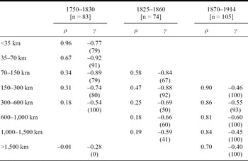
This procedure was repeated for other market pairs used in the correlation analysis, and the estimates for the indicators of interest (correlation, ρ, and the total error correction term, γ) have again been grouped according to distance and time period. In total, this estimation process was repeated for 262 market pairs—83 of which cover the period 1750–1830, 74 the period 1825–1860, and 105 the period 1870–1914.Footnote ²⁹ The results are shown in Table 5.

Table 5

ERROR CORRECTION MODELS

Notes:

Notes: n = total number of market pairs examined. Distance ranges with n ≤ 3 are not reported. Percentage of test statistics of γs significant at a 95 percent level are in parentheses (critical value of –2.86 from Dickey-Fuller distribution).

Sources:

See the text and the Appendix.

The general picture is strikingly similar to the correlation analysis. The estimates for both the correlation as well as the adjustment terms generally decrease with distance and increase over time. But caution is needed because the interpretation of the coefficients is not as straightforward as with the correlation analysis. The prime reason is that the co-movement of prices in different markets and the inter-annual price adjustments are not independent. First of all, one could conceivably have error correction without co-movement, but it would not be a sign of efficient market structures, but more likely the effect of uncorrelated local shocks that petered out over time. Second, the speed of adjustment could influence the co-movement of prices. That possibility is more likely with the sort of low-frequency data (annual) used here. If there is intensive year-round trade between two places, the co-movement between these prices will be higher than in a place where trade is limited. Moreover, the price differences after a shock in one place will in such cases not be fully detectable in an annual data series, as part of this difference will be corrected for by intra-annual arbitrage. One could therefore have a high degree of co-movement together with a moderate degree of inter-annual adjustment.

Fortunately, this last problem is not very likely to have affected the Indian results, at least in the late eighteenth and early nineteenth centuries. Trade was restricted to a few months, because the monsoon inhibited transport for much of the year. When looking at Table 5 we, in fact, do not see high co-movement of prices with relatively low adjustment. What we, instead, do see is a very low degree of co-movement for distances in excess of 70km, together with substantial adjustment terms, but again, such a combination is hardly a sign of well-integrated markets. For large distances, both the co-movement of prices and the adjustment to shocks become low and insignificant for the early period.

In the second period, the correlation and adjustment estimates suggest that market forces have spread beyond the local sphere, and up to distances of 300km, where we now find high and often significant adjustment terms alongside substantial co-movement. For larger distances, co-movement and adjustment are still very low and mostly insignificant.

As with correlation analysis, the picture changes radically when moving to the late nineteenth century. Now the co-movement of prices becomes very strong, not only for shorter distances, but even for places over 1,500km apart. At the same time, annual adjustments are now nearly always significant for all distances ranges. However, the adjustment coefficients have not increased and are only moderate for all distances.Footnote ³⁰ Here we likely have exactly the case outlined above, where intra-annual adjustment drives up the annual co-movement of prices but does not raise (or may even lower) the degree of inter-annual adjustments. Such an interpretation seems perfectly compatible with the emergence of a modern transport network in the late nineteenth century, which for the first time made year-round trade of bulky goods possible.

One last factor worth considering is whether the price shocks, which give rise to the adjustments, have actually declined in frequency and magnitude, especially in the late nineteenth century.Footnote ³¹ This is a concern because an error correction of 50 percent of a massive price differential is not the same thing as a 50 percent correction of a small error. Small errors are in fact much more likely to persist, even in well-integrated markets, for at some point the price difference may be lower than the total transaction costs, therefore providing no incentive for arbitrage.

Clearly, although it seems perfectly fine to use annual data for estimating error correction models for the late eighteenth century and the early nineteenth century, the limitations of such an approach for analyzing adjustment processes in late-nineteenth-century India become very apparent. A good part of the adjustment process seems now to fly below the radar provided by annual data.

In Europe the same problem will rear its head even earlier—and indeed throughout the entire period under study—because of the higher degree of integration. European markets have been analyzed by other scholars who estimated error correction models with higher frequency (weekly or monthly) data. Comparisons to, and among, these studies are not straightforward and not always very transparent. Not only do the data frequencies vary, but these models also come in many different specifications. Nonetheless, it is certainly possible to make a rough assessment of comparative market efficiency. Indeed, great precision is unnecessary because Europe and India were dramatically different. Already for late-seventeenth- and early-eighteenth-century France, Cormac O'Grada, and Jean-Michel Chevet find for cities of up to a distance range of about 250 km both co-movement of prices and fairly quick adjustment processes.Footnote ³² For very distant markets, however, the adjustment processes were still extremely slow up to the nineteenth century.Footnote ³³ This changes in the nineteenth century, and the “emergence of a truly international market for wheat” has recently been dated at around 1835.Footnote ³⁴ For this period, a moderate degree of co-movement and fairly fast adjustment processes are in India still restricted to distance ranges below 300km. Meanwhile in Europe, markets seem to have functioned pretty efficiently even during famine conditions.Footnote ³⁵ In the course of the revolutionary developments in transport and communication from the 1870s onwards, the pace of the integration increased yet more: By the late nineteenth century, adjustment processes to price differentials even between distant markets were down to a couple of weeks, not just across Europe but even between U.S. export centers and European cities.Footnote ³⁶

CONCOMITANTS OF INTEGRATING MARKETS: PRICE CONVERGENCE AND DECREASING PRICE VOLATILITY

In the process of market integration, domestic prices that were formerly independent of the world price are becoming more and more determined by the latter. It logically follows from the law of one price that in the process of such a transition there has to be a convergence of the prices towards a single price or—due to transport costs—to a stable price ratio. Commodity price convergence is in fact considered a reliable indicator for expanding markets, and history offers plenty of examples of convergence as a consequence of increased trade opportunities.Footnote ³⁷

Grain price series for the major regions of India from 1760 to 1914 confirm this assertion and provide a powerful illustration of how grain markets were integrated on the Indian subcontinent. Wheat price series have already been shown in Figure 2, and the corresponding rice price patterns are displayed in Figure 3.

Figure 3

CONVERGENCE OF RICE PRICES

Sources: See the Appendix.

In those two graphs, price levels were more or less stationary in all regions until about 1850, and prices for the same grain in different markets seemed to be totally unconnected: prolonged and massive differences in price levels were normal, price movements were asynchronous, and big price spikes did not coincide. The implication seems to be that distant grain markets remained fragmented until the 1850s.

In the following decade, price movements in different markets began to resemble one another, but the differences in the price levels were still rather big, a fact that can be explained by high freight rates.Footnote ³⁸ Around 1890 prices began to converge, and price differentials shrank. Apparently, a national grain market was forming at the turn of the twentieth century.

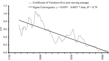
This process of price convergence stands out even more clearly if we condense the data into a single series, by plotting either the coefficient of variation or the so-called sigma convergence—the trend rate of decline of the coefficient of variation over time (Figure 4). For both indicators of convergence, the regional rice prices in Figure 3 have been used. Over periods as long as 150 years, the sigma convergence yields highly significant coefficients, evidence of how robust this trend is. As for the timing of the convergence, the coefficient of variation provides us with more precise information than Figure 3. There was a first drop in the price variation across regions is visible during the first two decades of the nineteenth century, and a second one starting in the 1870s and lasting up to the turn of the twentieth century, when prices were nearly equal across the subcontinent.

Figure 4

SIGMA CONVERGENCE

Sources: See the text and the Appendix.

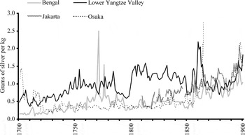
If we consider the larger international picture, it appears that the Indian national market for grain emerged around the same time as India became integrated into the Asian (or world) rice market. The leveling of prices in the Asian rice market emerges clearly in Figure 5, which presents long price series from different locations in Asia. Throughout the eighteenth and the first half of the nineteenth century, differences in price levels were pronounced, and short- and medium-term prices moved independently in India, China, Japan, and Indonesia. Rice in Bengal was mostly cheaper than in Indonesia, and much cheaper than in the Yangtze valley. Rice prices in Japan started at a very high level, but then decreased in the 1720s and generally remained the lowest there-after until the mid-nineteenth century. That was also when price gaps within Asia began to decrease substantially, and from the 1870s onwards price movements also started to resemble each other.Footnote ³⁹

Figure 5

CONVERGENCE OF RICE PRICES IN ASIA

Sources: See the text and the Appendix.

As Figure 5 suggests, it was not until the end of the nineteenth century that the rice trade in Asia was extensive enough to have a clear effect on prices across the continent. Judging by the extent of co-movements of prices, the degree of international integration was, however, not quite comparable to the national integration within India.Footnote ⁴⁰

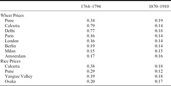
A second characteristic of an expanding market is lower price volatility. Volatility is normally lower in integrated markets because geographical arbitrage between surplus and deficient regions keeps large variations in the local harvest from translating into big price shocks.Footnote ⁴¹ The measure used here for price volatility is the coefficient of variation, and I have calculated it for some of the most important Indian markets in the late eighteenth and nineteenth centuries: the Mughal capital Delhi, the Maratha capital Pune, and Calcutta, the rising center of British power.Footnote ⁴²Table 6 shows that the wheat price volatility in these centers was massive in the second half of the eighteenth century, with an average annual price fluctuation of between 34 percent and 78 percent of the mean price. In the nineteenth century this changed dramatically so that the coefficients of variation fell below 20 percent in all three markets, suggesting a fundamentally different market structure. From the same table it becomes equally apparent that the situation in Europe at the time was very different. At the end of the eighteenth century, the wheat price volatility in Indian markets was about two to four times higher than in big European markets.

Table 6

COEFFICIENTS OF VARIATIONS

Sources:

See the text and the Appendix.

A comparison of these findings with David Jack's analysis of pre-modern European market integration suggests two things: First, the volatilities calculated for Europe and shown in Table 6 are comparable to the price volatilities he found for eighteenth-century Europe. Second, after 1500, wheat price volatility in major European markets was never as high as in late-eighteenth-century India.Footnote ⁴³ However, because price volatility only decreased modestly in nineteenth-century Europe, volatilities in India and Europe finally became comparable at the end of this century, even though prices in Pune and Delhi still fluctuated more than in any other city included in the sample.

A comparison of the price volatility of rice in India, China, and Japan shows a similar pattern. The coefficients for India are on average about 70 percent higher than in Osaka and the Yangtze valley in the late eighteenth century. But because volatility declined much more sharply in India thereafter, the figures for Pune and Calcutta are comparable by the late nineteenth century.Footnote ⁴⁴

POLITICAL AND ECONOMIC FRAGMENTATION, AND IMPERIAL INTEGRATION

The evidence I have assembled fits well with both the general history of India and traditional accounts of Indian market integration. Other than the revisionist work by Frank, Pomeranz, or K. N. Chaudhuri, this mainstream view contends that the emergence of integrated commodity markets in India—as opposed to markets for luxury or high-value goods—was a process that did not start until the second half of the nineteenth century. Before that time, it is argued, markets for most products (and for grain as a good with a high bulk-to-value ratio in particular) remained isolated due to high transportation costs and political fragmentation.Footnote ⁴⁵ Let us briefly review the grounds upon which these mainstream conclusions rest and sketch a historical narrative that can create a context for the quantitative analysis.

In the century following the accession of Akbar (1556), most of India experienced an epoch of relative peace, political stability, and prosperity, in which trade expanded and urban centers grew everywhere. This situation started to change, however, when, under Aurangzeb's reign (1658–1707), the Mughal empire expanded so much that it could hardly be ruled any longer. To finance his southern conquest, which had the aim of uniting northern and southern India under his rule, Aurangzeb made increasingly oppressive demands for revenue. That, in turn, triggered widespread peasant revolts that undercut political stability. After Aurangzeb's death, the short succession of weak Mughals aggravated the situation further and greatly weakened Mughal central power. In the 1730s, the Marathas raided both Delhi, the Mughal capital, and Surat, which subsequently lost its role as the great port of the empire within a few decades. While Mughal power was diminishing, regional powers began to struggle for supremacy over India, with the Afghans, the Marathas, and several Mughal governors being the main contenders. The Europeans remained marginal to the Indian political scene until the middle of the eighteenth century.

Not surprisingly, this decay of political stability and insecurity of life and property resulted in dwindling trade. Merchants became an easy target for robbers and government officers alike, while trade routes became increasingly unsafe or were disconnected altogether. Long-distance trade seems to have suffered most, and some regions were far more affected than others.Footnote ⁴⁶ Moreover, political regionalization led to the introduction of new duties, thus further lowering incentives to trade. A related development arising from this political fragmentation was the deterioration of the transport infrastructure—a factor crucial to any market structure.

In the seventeenth century, the Mughals had built and maintained a long-distance road network, which served both military purposes and commercial interests. With the decline of Mughal power, this system of built roads, which was already limited in geographic coverage and density, started to decay.Footnote ⁴⁷ The road network deteriorated even further with the rise of the Marathas, as they were primarily fighters and not concerned with the development of infrastructure. As a result, even the few built roads were in a terrible condition by the mid-eighteenth century; old highways were overgrown by jungle, and Mughal bridges, wells, and caravanserais were in ruin.Footnote ⁴⁸ Without adequate roads, it was impossible to use bullock carts in most cases, and all the goods for inland trade had to be transported on the backs of pack animals.Footnote ⁴⁹ In some regions not even bullock paths existed, so that all produce had to be carried on the head.Footnote ⁵⁰ Moreover, during the rainy season, all this overland transport came to a halt, and the internal traffic was almost at a complete stand-still.

Given the extremely poor state of inland transport, the prime way to transport goods over longer distances was by ship—either on navigable inland rivers or on the Indian Ocean. Though naturally navigable rivers provided by far the cheapest available transport, they were not abundant in India. Inland navigation was mostly confined to the Ganges river system and the Sind. In South India, there was very little inland navigation, and in western India, there were no navigable rivers at all. Also, river transport was “directional,” with downstream transport heavily outweighing upstream transport, and was highly seasonal due to the monsoon.Footnote ⁵¹

The extent of the Indian maritime trade is debated but seems to have been rather limited compared to the situation in Europe before, say, the mid-nineteenth century. At Surat, the great port of the Mughal empire, which experienced its greatest phase of expansion at the end of the seventeenth century right before the collapse of Mughal power, about 50 ships arrived every year during this period. In the same period, Amsterdam—one of the major ports in Europe—received about 3,000 ships each year.Footnote ⁵²

Estimates of shipping capacity for Mughal India are equally small. For annual long-distance trade in the Indian Ocean at the beginning of the seventeenth century, estimates range from 52,000 to 74,500 tons. The comparative figure for European shipping capacity is between half a million and one million tons.Footnote ⁵³

Given this very poor transport infrastructure, which resulted in very high transport costs and very limited transport capacities, it is hardly surprising that grain markets are widely believed to have been highly fragmented, and that inland grain trade was essentially local, so that “grain rarely reached the next regional markets, even in the presence of famines or rising prices.” People predominantly consumed local products, and only high-value and luxury goods were transported over longer distances.Footnote ⁵⁴ Even on ships, grain seems to have played only a minor role, as merchants primarily transported high value goods such as spices, cotton and silk piece goods, ivory, or sugar.Footnote ⁵⁵

Political and economic fragmentation, lack of security, and regular warfare in some parts of the subcontinent characterized the socio-economic climate for the rest of the century—hence the term “crises of the eighteenth century.”Footnote ⁵⁶ It was not until the battle for the supremacy in India had been decided that the political and economic stability on the subcontinent as a whole started to improve. The winner of this battle was, of course, the British East India Company, and it secured this position once it had decisively beaten the Marathas, the only serious remaining contenders, in their capital Pune in 1818.

Having established their military supremacy on the subcontinent, the British slowly united it politically and economically to a degree previously unknown. Their efforts eventually led to a level of commercial activity unprecedented on the subcontinent.Footnote ⁵⁷ Among the many obstacles to a flourishing economy that the British eradicated were all inland and town duties; they also introduced a universal measurement system and made the silver rupee the only legal tender.Footnote ⁵⁸ So when British India officially became a part of the English Empire in 1858, the subcontinent was politically unified under an uncontested central power, and it had a universal legal system, a single weight system, a single currency, and a single official language, and was free of any internal customs.

Equally important was the dramatic improvement in the means of transportation that ensued. Although in some regions substantial progress was already achieved over the first half of the century, road construction and maintenance on a larger scale only started around 1850.Footnote ⁵⁹ Subsequently, the construction went ahead at a great speed so that by the end of the nineteenth century there were about 37,000 miles of paved roads and 136,000 miles of unpaved roads in India. “Thus, from the roadless situation at the beginning of the British rule, India had made considerable progress to gain what was the barest minimum urgently necessary for the commercial prosperity of the country.”Footnote ⁶⁰

The other major development that radically improved India's transport infra structure—and it did occur very much at the same time as the improvement of the road network—was the construction of an extensive railway network. Aided by government guarantees that provided a secure 5 percent return on all capital invested in the construction, it went ahead at a very rapid pace indeed: by 1900, there were about 25,000 miles of railway tracks.Footnote ⁶¹ Railroads reduced freight rates for food grains by approximately 80 percent compared to rates for carts, and rendered bulk shipments for grains possible.Footnote ⁶²

Finally, shipping technology and shipping connections also improved decisively, with the quantity of shipped goods experiencing a big surge in the nineteenth century. In the course of this process, the volume of shipped grain not only surged greatly in absolute terms, but also increased dramatically in relative terms vis-à-vis other goods, so that grain became the leading export commodity by 1900.Footnote ⁶³

To sum up, the processes of political and economic integration during the nineteenth century, coupled with the rapid improvement of transport facilities in the second half of the century, fundamentally transformed commercial activity, leading to an unprecedented extent of trade in general, and of grain trade in particular. Previously highly fragmented markets became unified to such a degree that by the end of the century India not only had a national market for grain, but was integrated into the world markets for both rice and wheat.Footnote ⁶⁴