1. Introduction
Environmental challenges are inherently global, with causes that often transcend national boundaries and consequences that are rarely confined to specific regions. Even if environmental problems appear to be localized, the international flow of goods and the migration of production factors can spread the effects of these issues—along with the impact of the policies designed to address them—throughout the global economic network. Effective management of these challenges requires not only coordinated international policy efforts but also a deep understanding of the economic and spatial dynamics that influence how pollution and regulation impact firms and individuals across regions.
In the context of controlling and managing pollutant emissions, policymakers typically employ two main approaches: command-and-control (from now on CAC) and market-based instruments. The CAC approach involves the government or a similar authority imposing specific pollution reduction requirements, such as precise emission thresholds, and monitoring compliance (Schwarz, Reference Schwarz2017). While CAC policies provide clear directives and can rapidly address specific environmental problems (Tuladhar et al. Reference Tuladhar, Mankowski and Bernstein2014; Lamperti et al. Reference Lamperti, Napoletano and Roventini2020), they have notable disadvantages compared to market-based measures. Specifically, CAC policies often impose higher compliance costs on regulated firms and are less likely to encourage innovation (Swaney Reference Swaney1992; Acemoglu et al. Reference Acemoglu, Hanley, Akcigit and Kerr2016). Studies have shown that the rigid structure of CAC regulations can lead to ambiguous outcomes regarding firm growth and productivity, making it challenging to simultaneously achieve sustainable environmental outcomes and foster total factor productivity growth (Albrizio et al. Reference Albrizio, Kozluk and Zipperer2017; Hamamoto Reference Hamamoto2006; Gray and Shadbegian, Reference Gray and Shadbegian2003).
Environmental regulations can significantly influence the mobility of both individuals and firms. Empirical evidence consistently shows that individuals tend to relocate away from areas with high levels of pollution (Chen et al. Reference Chen, Ebenstein, Greenstone and Li2013, Reference Chen, Oliva and Zhang2022; Chay and Greenstone, Reference Chay and Greenstone2005). In contrast, firms may move away from regions with stringent environmental regulation due to the associated increase in operating costs. This behavior is captured by the Pollution Haven Hypothesis (from now on PHH), which specifically refers to firms’ tendency to concentrate in regions with more lenient environmental standards (Levinson and Taylor, Reference Levinson and Taylor2008). A growing body of empirical research supports this mechanism, showing that unilateral emission reduction policies can prompt the relocation of pollution-intensive activities to countries with weaker regulations, thereby reducing the overall effectiveness of such measures and potentially worsening global environmental outcomes (Batabyal, Reference Batabyal1996; Mulatu et al. Reference Mulatu, Gerlagh, Rigby and Wossink2010; Kheder and Zugravu, Reference Kheder and Zugravu2012; Martin et al. Reference Martin, Muûls, de Preux and Wagner2014; Schenker et al. Reference Schenker, Koesler and Löschel2018; Naumann et al. Reference Naumann, Bolz and Richter2022).
The PHH becomes more pronounced when environmental regulations are significantly stricter in one region or country compared to another. Studies such as Levinson and Taylor (Reference Levinson and Taylor2008) and Candau and Dienesch (Reference Candau and Dienesch2017) confirm that pollution-intensive industries are more likely to relocate to countries with weaker regulations, particularly when trade integration amplifies this effect. Similarly, Antoci et al. (Reference Antoci, Borghesi, Iannucci and Sodini2021) highlight that stricter emissions caps under the Emission Trading Scheme (ETS) not only increase allowance prices and promote emissions reduction but also intensify firm relocation, as companies follow profitable examples of other relocating firms. This trend is visible in developing and emerging economies, which often attract firms due to lower regulatory standards. Conversely, when regulatory differences are minimal, as observed within the EU, the PHH becomes less evident. In such cases, firms may lack strong incentives to relocate solely based on environmental regulation, as other factors such as innovation, labor costs, and market conditions may play a more significant role.
An alternative perspective is the Porter Hypothesis (from now on PH), which offers a more optimistic view on the role of stringent environmental policies. The PH argues that rather than harming competitiveness, strict environmental regulations can enhance a firm’s productivity and innovation capacity, thereby improving its long-term profitability and competitiveness. According to Porter and van der Linde (Reference Porter and van der Linde1995), well-designed environmental regulations can drive firms to explore more efficient production processes and adopt cleaner technologies, which can ultimately reduce costs, improve product quality, and open up new market opportunities. This is particularly evident for firms in the service sector and other non-heavily polluting industries (Jaffe et al. Reference Jaffe, Peterson, Portney and Stavins1995). This perspective challenges the conventional view that environmental regulation necessarily imposes a trade-off between environmental quality and economic performance.
The PH has gained considerable empirical support in recent years. For instance, Ambec et al. (Reference Ambec, Cohen, Elgie and Lanoie2013) provide a comprehensive review of empirical studies testing the PH, concluding that moderate environmental regulations often lead to “innovation offsets”—cost savings that arise from enhanced efficiency and productivity. These innovation offsets can fully or partially compensate for the costs of compliance, making stringent environmental policies more economically viable. Moreover, Costantini and Mazzanti (Reference Costantini and Mazzanti2012) show that environmental regulations can increase the export performance of green products, suggesting that such policies can help firms gain a competitive advantage in markets with growing demand for environmentally friendly goods and services. Other studies, such as Lanoie et al. (Reference Lanoie, Patry and Lajeunesse2011), find that firms subject to environmental regulations invest more in R&D and are more likely to develop innovative products and processes, further supporting the PH.
This paper aims to investigate how environmental regulation—in particular, a CAC measure aimed at reducing emissions in the industrial sector—can affect the long-run spatial distribution of people, capital, and pollution. The analysis explicitly considers the different motivations underlying the location decisions of individuals and firms, focusing on a two-region economy framework. We study the interactions between mobile firms, mobile households, and commodity trade to provide insights into the effectiveness of environmental regulations and the spatial dynamics they induce.
We employ a New Economic Geography (NEG) framework (Krugman, Reference Krugman1991) to study the complex interplay between environmental regulations, firm location decisions, and household mobility. This framework allows for a simultaneous examination of how local pollution and environmental policies influence the distribution of economic activities. Several studies in the NEG literature have explored the relationship between pollution and industrial location. For instance, van Marrewijk (Reference van Marrewijk2005) incorporates pollution as a local negative externality. The author introduces a damage function as a multiplicative term in the utility function, capturing the aversion effect of pollution on consumption. Lange and Quaas (Reference Lange and Quaas2007) find that when only industrial pollution is considered, it acts as a dispersion force. Ciucci et al. (Reference Ciucci, Prunetti and Maupertuis2015) analyze transboundary pollution and concludes that symmetric pollution with a local impact has a dispersion effect, while pollution that primarily affects another location acts as an agglomeration force. Caballero et al. (Reference Caballero, Martínez-García and Morales2024) investigate local pollution effects and factor migration, revealing “pollute-and-flee” cycles, where population and industry initially agglomerate but later disperse due to increasing local pollution.
Despite the extensive body of literature, few studies have explored the separate processes of household residence choices and firm mobility decisions. Rauscher (Reference Rauscher2009) and Rauscher and Barbier (Reference Rauscher and Barbier2010) investigate firms’ and households’ location decisions independently, considering the influence of factor remunerations and residential amenities. Borck et al. (Reference Borck, Pflüger and Wrede2010) study industrial location and residential choice as separate processes, finding equilibria with spatial separation between production and residential locations.
Our paper extends the analysis put forward by Commendatore et al. (Reference Commendatore, Kubin, Sodini and Sushko2024) by incorporating a CAC policy that requires firms to comply with a prescribed green technology standard. In addition, firms may receive subsidies (financed by a household tax). The analysis considers a two-region economy—where regions may also be interpreted as countries—comprising two sectors: agriculture and manufacturing. In agriculture, perfect competition prevails, while in manufacturing, monopolistic competition dominates. Two types of households live in the economy: workers and capital owners. Workers supply labor only locally, whereas capital owners may allocate their endowment of capital between the regions and are allowed to migrate across space.Footnote 1 Firms are homogeneous and emit pollutants with only local effects. When commodities are traded cross-border, iceberg trade costs are involved. The local government in one region imposes a technology standard on firms under its jurisdiction, increasing their fixed input requirement.
Our findings indicate that when environmental compliance costs are modest, firms are more inclined to locate in regions with stringent green standards. This supports the PH, but through a distinct mechanism: the expansion of local market size driven by the relocation of mobile households seeking cleaner environments.
However, when compliance costs become substantial, the pattern reverses. In line with the PHH, we observe a spatial divergence: households continue to favor cleaner regions for their environmental and health benefits, while firms relocate to areas with laxer regulations to avoid compliance costs.
Our findings align with empirical evidence from OECD industrial sectors (Wang et al. Reference Wang, Sun and Guo2019), which confirms that environmental policy boosts green productivity when stringency remains below a critical threshold. We contribute to this literature by highlighting market size as a complementary channel: environmental regulation can attract capital by enlarging local demand through household mobility, thereby reinforcing regional attractiveness.
Yet, once regulatory burdens exceed the benefits from market expansion, this advantage is lost. These results underscore the nuanced interaction between environmental regulation and the geography of economic activity, calling for balanced policy design that accounts for both firm behavior and household preferences.
2. The economic model
2.1 General Set-up
In this study, we consider an economic model composed of two symmetric regions, i.e., they share the same technology and consumer preferences and they have the same labor endowment (see below), denoted as Region 1 and Region 2. The model includes two key sectors: Agriculture (
 $A$
) and Manufacturing (
 $M$
), each of which plays a distinct role in the economy. The production process in these sectors relies on two primary factors of production: labor (
 $L$
) and capital (
 $K$
). The output of this economy consists of two corresponding goods: an agricultural good (
 $A$
) produced in the agricultural sector and a manufacturing good (
 $M$
) produced in the industrial sector.
Each firm in the manufacturing sector produces a single variety of the manufacturing good. In the absence of policy intervention, the production process requires each firm to employ
 $F$
units of
 $K$
and
 $\varsigma$
units of labor for each additional unit of output produced. With an environmental policy that we assume to be implemented only in Region 1, additional
 $\theta F$
units of the fixed input are required per firm, thereby increasing production costs. These
 $\theta F$
units contribute to the abatement of pollution emissions, and
 $\theta$
is a parameter fixed by the local government in Region 1 aiming to achieve some “green” standard. The wage rate of workers is denoted by
 $w$
, while the remuneration for one unit of
 $K$
is represented by
 $r$
.
The economy is populated by two types of households: workers (
 $L$
) and capital owners (
 $E$
). Capital owners are allowed to move between regions. The number of capital owners residing in Region 1 is
 $E_1$
, while those in Region 2 are
 $E_2$
. The per capita endowment of
 $K$
for each capital owner is given by
 $k = \frac {K}{E}$
. Capital is distributed between the two regions, with
 $\eta$
representing the share of total capital allocated to Region 1. Consequently,
 $1-\eta$
denotes the share allocated to Region 2. The spatial distribution of capital owners between the two regions is captured by the parameter
 $\lambda$
, which denotes the share of capital owners living in Region 1. Thus,
 $1-\lambda$
represents the share of capital owners living in Region 2, leading to
 $E_1 = \lambda E$
and
 $E_2 = (1-\lambda )E$
. Capital is sector-specific, while workers supply labor to both sectors
 $ A$
and
 $ M$
. The workforce is equally distributed between the two areas, with each region containing
 $\frac {L}{2}$
workers. These workers are assumed to be perfectly mobile between sectors but geographically immobile.Footnote
2
2.2 Consumption
The representative consumer’s utility function is given by:
 \begin{align} U(c_M, c_A, \varepsilon ) = u(c_M, c_A) - D(\varepsilon ), \end{align}
where
 $ u(c_M, c_A)$
represents the utility derived from consuming the manufacturing good and the agricultural good. Specifically,
 $ c_M$
is the consumption of a composite of manufacturing good varieties, and
 $ c_A$
is the consumption of the agricultural good. Moreover,
 $D(\varepsilon )$
captures the externality imposed by pollution on agents, who lack any direct means to control or mitigate their own exposure. Following Rauscher (Reference Rauscher2009) and Commendatore et al. (Reference Commendatore, Kubin, Sodini and Sushko2024), we assume a quasi-linear utility function:
 \begin{align} u(c_M, c_A) = c_M + c_A. \end{align}
The manufacturing good component
 $ c_M$
corresponds to:
 \begin{align} c_M = \Phi \left ( \sum _{i=1}^{N} c_i^{\frac {\sigma -1}{\sigma }} \right ), \end{align}
where
 $\sigma \gt 1$
represents the elasticity of substitution,Footnote
3
 $c_i$
the consumption of variety
 $i$
, and
 $\Phi \gt 0$
is a scaling parameter. The specification in (3) is the simplest way to capture love-of-variety à la Dixit and Stiglitz (Reference Dixit and Stiglitz1977). This assumption simplifies the analysis and allows for more analytical results. Its main implication is that individual demand is independent of both individual income and the price index, thereby neglecting income effects and interactions among differentiated goods.
The utility maximization problem is solved subject to the budget constraint:
 \begin{align} \sum _{i=1}^{n}p_i c_i + p_Ac_{A} = Y + p_A\overline {c_{A}}, \end{align}
where
 $p_i$
corresponds to the price of variety
 $i$
(with
 $i = 1, \ldots , N$
),
 $p_A$
is the price of the agricultural good,
 $Y$
is the income of an individual consumer (worker or capital owner), that may include local taxation, and
 $\overline {c_{A}}$
is a given endowment of the agricultural good. Moreover, as it is conventional in NEG models, we choose the agricultural good as the numéraire, giving
 $p_A = 1$
. We obtain the demand for a single variety
 $ i$
:
 \begin{equation*} c_i = \frac {\alpha }{p^\sigma _i}, \end{equation*}
where
 $\alpha = (\Phi \frac {\sigma -1}{\sigma })^\sigma$
. Note that since we are not yet considering space, in this expression there is not distinction between the price of a locally produced variety and the price of an imported one.
2.3 Production
In the absence of any environmental policy, the total number of firms in the economy is given by
 $N = \frac {K}{F}$
, where
 $K$
denotes the aggregate capital stock and
 $F$
the fixed capital requirement per firm. Firms are distributed across the two regions according to the capital share parameter
 $\eta$
, so that Region 1 hosts
 $N_1 = \frac {\eta K}{F}$
firms, and Region 2 hosts
 $N_2 = \frac {(1-\eta )K}{F}$
firms.
To introduce environmental regulation into the model, we consider a CAC policy implemented in Region 1 that mandates the adoption of cleaner production technologies to achieve a targeted reduction in emissions. This policy increases the amount of capital required per firm to operate, effectively increasing the fixed input requirement. We denote the stringency of the policy by the parameter
 $\theta \geq 0$
, which captures the increase in capital intensity due to compliance with environmental standards. A higher
 $\theta$
reflects more stringent requirements.
Consequently, the number of firms that can be supported in Region 1 becomes
 $N_1 = \frac {\eta K}{(1+\theta )F}$
while the number of firms in Region 2 remains unchanged at
 $N_2 = \frac {(1-\eta )K}{F}$
. The total number of firms in the economy is therefore:
 \begin{equation*} N = \frac {K}{F} \left ( 1 - \eta \frac {\theta }{1+\theta } \right ). \end{equation*}
As expected, the overall number of firms declines with the stringency of environmental policy, since a higher
 $\theta$
increases the fixed input requirement in the regulated region.Footnote
4
The production structure adheres to the footloose capital (FC) framework as outlined by Martin and Rogers (Reference Martin and Rogers1995). In this framework, the mobile factor, capital, contributes to production only as a fixed component. The profit of a representative firm, disregarding the location, is given by
 \begin{equation*} \pi = pq - (\varsigma qw + Fr), \end{equation*}
where
 $ q$
represents the output,
 $ \varsigma$
is the variable input requirement,
 $ F$
denotes the fixed amount of capital required for production,
 $ w$
is the nominal wage of workers, and
 $ r$
is the remuneration for capital. Moreover, following from perfect competition in the agricultural market and from mobility of workers between the sectors:
 $w = p_A = 1$
. With the introduction of environmental policy, regional profits
 $\pi _1$
for Region 1 and
 $\pi _2$
for Region 2 at the individual firm level are defined as:
 \begin{align}\pi _{1} & =(p_{11}-\varsigma )q_{11}+(p_{12}-\varsigma )\tau q_{12} -r_{1}(1+\theta )F+s,\end{align}
 \begin{align}\pi _{2} & =(p_{21}-\varsigma )\tau q_{21}+(p_{22}-\varsigma )q_{22}-r_{2}F,\end{align}
where
 $\tau \gt 1$
denotes the trade cost of the
 $M$
-good between regions, following the standard iceberg formulation,Footnote
5
 $ p_{ij}$
denotes the mill price charged in region
 $ j$
by a firm located in region
 $ i$
,
 $ q_{ij}$
represents the quantity sold in region
 $ j$
by a firm located in region
 $ i$
,
 $r_j$
indicates the remuneration for capital in region
 $ j$
and
 $s$
the subsidy paid to a firm in region 1, with
 $ i, j = 1, 2$
.
Market clearing for manufacturing good varieties requires:
 \begin{align*} q_{1,1} &= c_{1,1} \left ( \frac {L}{2} + \lambda E \right ), \qquad q_{1,2} = c_{1,2} \left ( \frac {L}{2} + (1 - \lambda ) E \right ), \\[5pt] q_{2,1} &= c_{2,1} \left ( \frac {L}{2} + \lambda E \right ), \qquad q_{2,2} = c_{2,2} \left ( \frac {L}{2} + (1 - \lambda ) E \right ). \end{align*}
Inserting these conditions in the above expressions for the regional profits and, finally, taking into account that prices at destination include trade costs:
 \begin{align}c_{1,1} &= \alpha p_{1,1}^{-\sigma }, \hspace {0.8 cm} c_{1,2} = \alpha p_{1,2}^{-\sigma }\tau ^{-\sigma },\end{align}
 \begin{align}c_{2,1} &= \alpha p_{2,1}^{-\sigma }\tau ^{-\sigma }, c_{2,2} = \alpha p_{2,2}^{-\sigma },\end{align}
we obtain the profit maximizing (mill) prices:
 $p_{i,j}=\frac {\sigma }{\sigma -1}\varsigma$
, where
 $\frac {\sigma }{\sigma -1}$
is the mark-up. It gives
 $p_{i,j}=1$
after setting for simplicity
 $\varsigma =\frac {\sigma -1}{\sigma }$
, with
 $i,j = 1, 2$
.
2.4 Subsidies and Taxation
The government in Region 1 may decide to pay a subsidy to firms to implement the green technology, breaking the symmetry between the two regions. These subsidies correspond to a fraction
 $0\leq x\leq 1$
of the cost increase suffered by a firm located in Region 1:
 \begin{equation} s=x\theta Fr_1. \end{equation}
Notice that the government knows the exact value of
 $s$
which is calculated at the short-run equilibrium. The subsidy is financed by an income tax (
 $tax$
) imposed on resident households. Thus the income of a representative household living in Region
 $i=1,2$
corresponds to
 \begin{align*} & Y_{1}+\overline {c_{A}}-tax\\[5pt] & Y_{2}+\overline {c_{A}}, \end{align*}
where
 $tax$
 \begin{align} tax =\frac {N_{1}}{\frac {L}{2}+E_{1}}s=\frac {\eta \frac {K}{(1+\theta )F}}{\frac {L}{2}+E_{1}}s=\frac {\eta K}{\frac {L}{2}+\lambda E} \frac {\theta }{1+\theta }xr_1. \end{align}
In essence, the total taxation in Region 1 is determined by the number of firms, workers, and capital owners located in the region, along with the subsidy set by the government to finance the environmental policy. We take
 $x$
as policy parameter.
2.5 Pollution
Emissions are proportional to production. To incorporate the (negative) effect of the green technology on emissions per unit of output we set:
 \begin{align}\varepsilon _{1} & =\frac {1}{1+\theta }N_{1}q_{1},\end{align}
 \begin{align}\varepsilon _{2} & =N_{2}q_{2},\end{align}
where
 $q_{1}=q_{11}+\tau q_{12}$
and
 $q_{2}=\tau q_{21}+q_{22}$
. The damage function
 $ D(\varepsilon )$
, that enters in the utility function additively, captures the negative impact on utility from industrial pollution emissions,
 $ \varepsilon$
:
 \begin{align} D(\varepsilon ) = \frac {\delta }{2} \varepsilon ^2, \end{align}
where
 $ \delta \geq 0$
represents the intensity of the pollution effect on utility.Footnote
6
3. Short-run equilibrium
In the short-run equilibrium, we determine regional returns to capital and indirect utilities for capital owners that ensure equilibrium in both goods and labor markets, based on fixed distributions of households and firms as represented by
 $\lambda$
and
 $\eta$
, respectively. As we will show, these differences in remuneration and utility play a central role in driving the long-run dynamics.
3.1 Regional Capital Remunerations
Starting from the zero-profit conditions (obtained by setting
 $\pi _1 = 0$
and
 $\pi _2 = 0$
in equations (5) and (6) and substituting the profit-maximizing prices) we derive the short-run equilibrium values for regional capital returns:
 \begin{align}r_1 &= \frac {1}{\sigma F[1 + (1 - x)\theta ]} q_1 \notag \\[5pt] &= \frac {\alpha }{\sigma F[1 + (1 - x)\theta ]} \left ( \frac {L}{2} + \lambda E + \phi \left ( \frac {L}{2} + (1 - \lambda ) E \right )\right ),\end{align}
 \begin{align}r_2 &= \frac {1}{\sigma F} q_2 = \frac {\alpha }{\sigma F} \left ( \phi \left ( \frac {L}{2} + \lambda E \right ) + \frac {L}{2} + (1 - \lambda ) E \right ).\end{align}
where we used the standard definition of trade freeness
 $\phi = \tau ^{1 - \sigma }$
, with
 $0 \leq \phi \lt 1$
. Notice that
 $r_1$
and
 $r_2$
depend on the market size (determined by
 $\lambda$
) and production costs (affected by the policy
 $\theta$
), and they do not depend on local competition (determined by
 $\eta$
).
3.2 Capital Owner Regional Indirect Utilities
From (1) and (2), the utility of a representative capital owner living in Region 1 and in Region 2, respectively, is given by:
 \begin{align*} u_1(c_{M,1}, c_A, \varepsilon _{1}) &= c_{M,1} + c_A - D(\varepsilon _{1})\\[5pt] u_2(c_{M,2}, c_A, \varepsilon _{2}) &= c_{M,2} + c_A - D(\varepsilon _{2}), \end{align*}
where from (3),
 \begin{align*} c_{M,1} &= \Phi \left ( N_{1} c_{1,1}^{\frac {\sigma -1}{\sigma }} + N_{2} c_{2,1}^{\frac {\sigma -1}{\sigma }} \right )\\[5pt] c_{M,2} &= \Phi \left ( N_{1} c_{1,2}^{\frac {\sigma -1}{\sigma }} + N_{2} c_{2,2}^{\frac {\sigma -1}{\sigma }} \right ), \end{align*}
and from (13),
 \begin{align*} D(\varepsilon _1) = \frac {\delta }{2} \varepsilon _1^2,\\[5pt] D(\varepsilon _2) = \frac {\delta }{2} \varepsilon _2^2 .\end{align*}
Replacing for utility maximizing consumption, considering (7) and (8) and that
 $p_{ij} = 1$
with
 $(i,j =1,2)$
,
 $\alpha = (\Phi \frac {\sigma -1}{\sigma })^\sigma$
,
 $N_1 = \frac {\eta }{1+\theta } \frac {K}{F}$
and
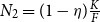 $N_{2} = (1 - \eta ) \frac {K}{F}$
, the indirect utilities correspond to:
 \begin{align}u_1 &= \frac {\alpha \sigma }{\sigma - 1} \frac {K}{F} \left ( \frac {\eta }{1 + \theta } + \phi (1 - \eta ) \right ) + c_A - \frac {\delta }{2} \varepsilon _1^2,\end{align}
 \begin{align}u_2 &= \frac {\alpha \sigma }{\sigma - 1} \frac {K}{F} \left ( \phi \frac {\eta }{1 + \theta } + 1 - \eta \right ) + c_A - \frac {\delta }{2} \varepsilon _2^2.\end{align}
Observe that the first component of the indirect utilities, representing the consumption of the manufacturing good, is influenced by the allocation of firms across regions. When a larger share of product varieties is locally available, avoiding transport costs and thus reducing prices, the utility level increases. This reflects the impact of regional product availability on the cost of living and overall utility, which we refer to as the cost of living effect. Using the budget constraint (4) solved for
 $c_{A}$
and expressions (11), (12), (14) and (15), we obtain:
 \begin{align}u_{1} & =\overline {r}k-tax+\overline {c_{A}}+\left [\frac {\alpha }{\sigma -1}\frac {K}{F}\left ( \frac {\eta }{1+\theta }+\phi \left ( 1-\eta \right ) \right )\right ] -\frac {\delta }{2}\varepsilon _{1}^{2},\end{align}
 \begin{align}u_{2} & =\overline {r}k+\overline {c_{A}}+\left [\frac {\alpha }{\sigma -1}\frac {K}{F}\left ( \phi \left ( \frac {\eta }{1+\theta }\right ) +1-\eta \right )\right ] -\frac {\delta }{2}\varepsilon _{2}^{2},\end{align}
where
 $\overline {r}=\eta r_{1}+(1-\eta )r_{2}$
represents the average remuneration of a unit of capital.
4. Long-run dynamics
4.1 The Dynamic Map
We assume that the mobility decisions of households and firms (the latter through capital allocation choices) are governed by an adaptive mechanism resembling replicator dynamics, a framework widely used in evolutionary game theory (Weibull, Reference Weibull1995) and commonly applied in NEG models (Fujita et al. Reference Fujita, Krugman and Venables1999; Baldwin et al. Reference Baldwin, Forslid, Martin, Ottaviano and Robert-Nicoud2003). The adoption of evolutionary dynamics is justified as it captures empirically observed patterns of relocation behavior. Firms tend to gradually relocate toward regions offering higher short-term returns, consistent with empirical evidence on firm responses to environmental and cost differentials (Eskeland and Harrison, Reference Eskeland and Harrison2003). Similarly, households migrate in response to current utility differentials, in line with documented evidence of pollution-induced mobility (Chen et al. Reference Chen, Oliva and Zhang2022). Furthermore, evolutionary dynamics account for cognitive and informational constraints, in accordance with the notion of bounded rationality. Firms often lack the capacity to fully anticipate the long-term effects of environmental policy interventions (Dosi and Nelson, Reference Dosi and Nelson1994), while households tend to react myopically to pollution exposure—relocating ex post rather than engaging in anticipatory migration—consistent with adaptive residential mobility models (Mulder, Reference Mulder1996).
Formally, the share of households residing in Region 1 (and, conversely, in Region 2) evolves according to the short-term utility differential
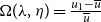 $\Omega (\lambda ,\eta )=\frac {u_{1}-\overline {u}}{\overline {u}}$
as follows:
 \begin{equation*} f(\lambda ,\eta )=\lambda \left ( 1+\gamma _{\lambda }\Omega (\lambda ,\eta )\right ) \text{,} \end{equation*}
where
 $\overline {u}=\lambda u_{1}+(1-\lambda )u_{2}$
and
 $\gamma _{\lambda }$
is the adjustment speed of household migration; and capital allocation depends on the short-term remuneration differential
 $\Psi (\lambda ,\eta )=\frac {r_{1}-\overline {r}}{\overline {r}}$
as follows:
 \begin{equation*} g(\lambda ,\eta )=\eta \left ( 1+\gamma _{\eta }\Psi (\lambda ,\eta )\right ) \text{,} \end{equation*}
where
 $\gamma _{\eta }$
is the adjustment speed of firms mobility. After introducing the constraints on shares that typically characterize NEG models, the 2-D map governing the discrete-time evolution of the two main variables,
 $\lambda$
and
 $\eta$
, corresponds to
 \begin{equation*} T:(\lambda ,\eta )\rightarrow (F(\lambda ,\eta ),G(\lambda ,\eta )), \end{equation*}
where
 \begin{eqnarray*} F(\lambda ,\eta ) &=&\left \{ \begin{array}{ccc} 0 &\quad if &\quad f(\lambda ,\eta )\leq 0 \\ f(\lambda ,\eta ) &\quad if &\quad 0\lt f(\lambda ,\eta )\lt 1 \\ 1 &\quad if &\quad f(\lambda ,\eta )\geq 1\end{array}\right . \\[5pt] G(\lambda ,\eta ) &=&\left \{ \begin{array}{ccc} 0 &\quad if &\quad g(\lambda ,\eta )\leq 0 \\ g(\lambda ,\eta ) &\quad if &\quad 0\lt g(\lambda ,\eta )\lt 1 \\ 1 &\quad if &\quad g(\lambda ,\eta )\geq 1.\end{array}\right . \end{eqnarray*}
The
 $2$
-D map
 $T$
has a piecewise smooth definition with flat branches. It fully describes the dynamics of the two main state variables describing the evolution of the economic system: the regional shares of capital owners (
 $\lambda$
) and capital (
 $\eta$
). Its domain corresponds to the unit square
 $U=[0,1]\times \lbrack 0,1]$
.
4.2 Long-Run Stationary Equilibria (Map T Fixed Points)
The long-run stationary equilibria of the dynamic model correspond to the fixed points of map
 $T$
. Due to the constraints on the shares, which confine the dynamics of the map within the unit square
 $u$
, we identify three types of fixed points:
-
• Interior equilibria, located in the interior of
 $U$
;
-
• Border equilibria, located at the interior points of the sides of
$U$
; -
• Core-Periphery equilibria located on the corners of
$U$
.


Now we give more details starting from the interior fixed points. From
 $f(\lambda , \eta ) = \lambda$
and
 $g(\lambda , \eta ) = \eta$
, we deduce that an interior fixed point satisfies the following conditions:
 \begin{equation} r_1(\lambda ) = r_2(\lambda ) ,\end{equation}
 \begin{equation} u_1(\lambda , \eta ) = u_2(\lambda , \eta ) ,\end{equation}
which imply equal regional capital returns (Equation (20)) and equal mobile households utilities across space (Equation (21)), respectively. There are at most two interior equilibria, which we denote
 $I_1 = (\lambda , \eta _1)$
and
 $I_2 = (\lambda , \eta _2)$
, where
 $\lambda$
directly solves the first of the above equations. The expressions for
 $\lambda$
,
 $\eta _1$
and
 $\eta _2$
, given their length, are reported in Appendices A1 and A2. Moreover, in those Appendices, we show conditions under which
 $I_1$
and
 $I_2$
exist. An important feature of interior equilibria is that both firms and mobile households are spread across countries. This distribution is asymmetric, except when neither region implements an environmental policy, as in Commendatore et al. (Reference Commendatore, Kubin, Sodini and Sushko2024).
We now consider the border fixed points. First, no equilibria can exist in the interior of the vertical borders of
 $U$
, for which
 $\lambda = 0$
and
 $\lambda = 1$
, as these values cannot satisfy equation (20).Footnote
7
The economic intuition behind is as follows: according to equations (14) and (15), the regional returns depend on the distribution of demand, weighted by the transport costs. When demand is fully concentrated in one region,
 $\lambda = 0$
or
 $\lambda = 1$
, firms in each region face different demand conditions, translating into different remunerations. Equal demand conditions, and hence equal remuneration, can only occur when equation (20) holds. Looking at the interior of the horizontal borders of
 $u$
, for which
 $\eta = 0$
or
 $\eta = 1$
, these are obtained by solving for
 $\lambda$
equation (21) after setting
 $\eta = 0$
and
 $\eta = 1$
, respectively. Again the explicit solutions, given their length, are provided in Appendix A3. In that Appendix, it is also shown that only one feasible equilibrium, denoted as
 $B$
, can exist on the lower horizontal border (
 $\eta =0$
). In the Appendix A3, it is also suggested that at most two feasible equilibria can exist on the upper horizontal border (
 $\eta =1$
). For the parameter combination we chose below for our numerical simulations, only one of these border equilibria exists, denoted as
 $B'$
. The economic interest of these equilibria is that when
 $\eta = 0$
or
 $\eta = 1$
, firms are concentrated in one region while capital owners are spread across space.
Finally, the Core-Periphery equilibria at the corners of the unit square always exist. These are denoted as
 $CP_{00} = (0,0)$
,
 $CP_{01} = (0,1)$
,
 $CP_{10} = (1,0)$
,
 $CP_{11} = (1,1)$
. From an economic perspective, recall that at the equilibria
 $CP_{00}$
and
 $CP_{11}$
, we encounter an extreme case in which both firms and capital owners are entirely concentrated in the same region. The equilibria
 $CP_{01}$
and
 $CP_{10}$
describe situations where firms concentrate in one region while all capital owners reside in the other.
Crucially, the existence and stability properties of the fixed points depend on the parameter configuration.Footnote
8
To deepen our analysis on the role of environmental regulation—focusing in particular on the impact of the parameter
 $\theta$
—it is essential to complement the exploration of these properties numerically. To this end, we adopt the following parameter set:Footnote
9
 \begin{align*} \sigma &= 3,\quad E = 1,\quad K = 1,\quad L = 2,\quad F = 0.05, \\[5pt] \alpha &= 0.1,\quad \gamma _\lambda = 2,\quad \gamma _\eta = 2,\quad \delta = 0.1, \\[5pt] \bar {c}_A &= 1,\quad \phi = 0.35,\quad x = 0.2,\quad \theta \in [0, 0.5].\\[-20pt]\nonumber \end{align*}
In Figure 1 we present a diagram—called bifurcation diagram—showing the behavior of the fixed points of map
 $T$
by increasing
 $\theta$
in the interval
 $[0, 0.5]$
within the feasible range of
 $\lambda$
and
 $\eta$
, i.e.
 $[0,1]$
. Solid lines correspond to a locally stable fixed point, while dashed lines correspond to an unstable fixed point. When curves cross at a specific point—a so-called bifurcation point—the properties of the fixed points involved change. In Figure 1, both interior equilibria
 $I_1$
and
 $I_2$
are visible. Considering the equilibrium
 $I_1$
, it is always stable within the feasible range. Increasing sufficiently
 $\theta$
, it eventually disappears leaving the feasible range of
 $\eta$
at the bifurcation point
 $T_1$
(where
 $\eta = 0$
), where it crosses the border equilibrium
 $B$
. Interestingly, at
 $T_1$
, the equilibrium
 $B$
gains stability.Footnote
10
Concerning the interior equilibrium
 $I_2$
, it is always unstable. When
 $I_2$
enters the feasible range (
 $\lambda = 1$
) at the bifurcation point
 $T_2$
, it crosses the border equilibrium
 $B'$
. After
 $T_2$
,
 $B'$
becomes locally stable. This equilibrium loses stability at the bifurcation point
 $T_3$
, where the Core-Periphery equilibrium
 $CP_{11}$
becomes locally stable. Finally, when
 $\theta$
becomes sufficiently large.Footnote
11
 $I_2$
exits the feasible range and the Core-Periphery equilibrium
 $CP_{11}$
loses stability at the bifurcation point
 $T_4$
.Footnote
12
Bifurcation diagram of
 $\lambda$
and
 $\eta$
with respect to
 $\theta$
, showing the long-run stationary equilibria and their properties for the chosen parameter constellation.

According to Figure 1, there are values of the parameter
 $\theta$
for which more than one equilibrium is locally stable---that is, multiple attractors coexist. This is a notable property of dynamical systems, as it implies that history matters: the long-run equilibrium outcome depends on the initial conditions. In the context of our model, the initial spatial distribution of capital owners and firms can influence where industrial activities and mobile households ultimately locate. To clarify this aspect, we illustrate in Figure 2 how the basins of attraction of the fixed points of the map
 $T$
evolve as the parameter
 $\theta$
increases, that is, at different levels of policy regulation. The basin of attraction of an equilibrium comprises all initial conditions from which the system’s state variables,
 $\lambda$
and
 $\eta$
, will eventually converge to that equilibrium.
Figure 2 is based on the same parameter combination introduced above and is plotted for six values of
 $\theta$
(0, 0.1, 0.2, 0.25, 0.4, and 0.5), representing different intensities of policy regulation. The fixed points appearing in the various panels of Figure 2 are the same as those plotted in Figure 1. The interior equilibria (
 $I_1$
and
 $I_2$
) are determined by the intersection of the line
 $\Psi$
, which plots equation (20) in the
 $(\lambda , \eta )$
plane, and the curve
 $\Omega$
, which plots equation (21) in the same plane. The border equilibrium
 $B'$
is defined by the intersection of the curve
 $\Omega$
with the upper boundary of the unit square
 $U$
(where
 $\eta = 1$
), while the border equilibrium
 $B$
is defined by its intersection with the lower boundary (where
 $\eta = 0$
). Locally stable fixed points are represented by black dots and unstable ones by white dots.
Starting from Figure 2a, in this scenario with no policy regulation,
 $\theta = 0$
, only the interior equilibrium
 $I_1$
exists representing the global attractor for the dynamics starting from the interior points of
 $U$
, with the corresponding basin of attraction colored in yellow. When
 $\theta = 0$
the interior equilibrium involves a symmetric distribution of capital and capital owners between the two countries.
When the stringency of the policy is low—as in Figure 2b where
 $\theta = 0.1$
—
 $I_1$
remains the only stable equilibrium, but symmetry is broken. The environmental policy affects both households and firms through two distinct channels. Specifically, in Region 1, where the policy is implemented, both the share of capital and the proportion of capital owners increase.Footnote
13
This scenario can be described as a moderate policy intervention. As long as the expansion of market size in Region 1 outweighs the cost burden imposed by the environmental regulation, this region continues to attract an increasing share of capital.
As
 $\theta$
is further increased, as shown in Figure 2c, where
 $\theta = 0.2$
, an interesting scenario emerges. The bifurcation at point
 $T_2$
(see Figure 1) has occurred: the interior equilibrium
 $I_2$
now exists, and the border equilibrium
 $B'$
has become stable. In this configuration, two attracting fixed points coexist: the interior equilibrium
 $I_1$
and the boundary equilibrium
 $B'$
(located on the side where
 $\eta = 1$
). The basin of attraction for
 $I_1$
appears as a yellow tongue, while the brown region represents initial conditions that converge to
 $B'$
. In this context, as noted earlier, “history matters”: initial conditions dictate which long-run equilibrium the system will reach. If the initial state lies within the basin of attraction of
 $I_1$
, the system converges to an interior equilibrium where less than 40% of capital and approximately 70% of capital owners are located in Region 1. Conversely, if the initial state lies within the basin of attraction of
 $B'$
, the system converges to a near-corner solution where nearly all capital and almost the entire population of capital owners are concentrated in Region 1.
This coexistence of stable equilibria also opens the possibility of path dependence driven by shocks: a sufficiently large disturbance that shifts the initial values of
 $\lambda$
and
 $\eta$
from one basin of attraction to another can lead to a dramatically different long-run spatial distribution of industry and households.
Figure 2d, where
 $\theta = 0.25$
, displays a structure similar to that of Figure 2c, with two distinct stable equilibria. However, the bifurcation point
 $T_3$
(see Figure 1) has now been crossed: the border equilibrium
 $B'$
has disappeared, and the Core-Periphery equilibrium
 $CP_{11}$
has gained stability. The basin of attraction, represented by the grey region, includes all initial conditions that converge to this equilibrium. In
 $CP_{11}$
, not only is all industry concentrated in Region 1, but all capital owners are located there as well.
Basins of attraction of the locally stable fixed points as the parameter
 $\theta$
varies. Black dots indicate locally stable fixed points, white dots represent unstable fixed points.

In Figure 2e, with a further increase in
 $\theta$
to a relatively high value (
 $\theta = 0.4$
), the system reaches a configuration beyond the bifurcation point
 $T_1$
(see Figure 1). The interior fixed point
 $I_1$
has collided with the lower boundary of the unit square
 $U$
(where
 $\eta = 0$
) and crossed the border equilibrium
 $B$
. As a result,
 $I_1$
disappears and
 $B$
gains stability, with the basin of attraction of this equilibrium colored in magenta. In this scenario, the only stable fixed points lie on the boundaries of
 $U$
: the Core-Periphery equilibrium
 $CP_{11}$
, located at the corner of
 $U$
, and the border equilibrium
 $B$
, located on the line
 $\eta = 0$
. In the first equilibrium, all capital and all capital owners are concentrated in Region 1. In the second equilibrium, all capital is located in Region 2, while nearly all capital owners remain in Region 1.
Finally, in Figure 2f, we return to a configuration with a single stable equilibrium: the border equilibrium
 $B$
at
 $\eta = 0$
. At this high level of regulation (
 $\theta = 0.5$
), all other equilibria have vanished or lost stability (see Figure 1 beyond the bifurcation point T4). In this outcome, all capital is located in Region 2, while nearly all capital owners remain in Region 1. The entire set of initial conditions falls within the basin of attraction of
 $B$
, shown in magenta.
5. Economic discussion
In this section, we examine the behavior of the stable stationary equilibria with respect to
 $\theta$
, with particular focus on the stable interior equilibrium
 $I_1$
. The impact of
 $\theta$
on
 $I_1$
is illustrated in the two panels of Figure 3. Several key insights emerge, with two distinct scenarios unfolding depending on the value of
 $\theta$
.
We begin by considering the population size (
 $\lambda$
) in Region 1. As
 $\theta$
increases, we observe a consistent upward trend (illustrated by the blue line in Figure 3). This trend is largely driven by the benefits of reduced pollution (resulting from environmental policy and a decline in the number of—polluting—firms, see Figure 4), which enhance the region’s attractiveness.
(a) Evolution of the stable interior equilibrium
 $I_{1}$
as
 $\theta$
varies. (b) Magnified view of (a): inverted u-shaped behavior of
 $\eta$
.

Turning to the share of capital, we observe two distinct scenarios: In scenario 1, when
 $\theta$
is relatively low (
 $\theta$
<0.095), an increase in
 $\theta$
attracts capital (
 $\eta$
) (represented by the red line in Figure 3) to the region adopting green technology standards. This shift is driven by the expanding population and, consequently, by the broadening of market size, associated with stricter environmental regulations.
In scenario 2, when
 $ \theta$
is relatively large (
 $ \theta$
> 0.095), the pattern reverses (see Figure 3). As the green technology standards become more stringent, capital (
 $\eta$
) reallocates from the green-technology region (Region 1) to the more polluted one (Region 2). In this case, the rising fixed costs associated with stricter standards in Region 1 outweighs the benefits of a larger market, creating strong incentives for capital to relocate to Region 2.
Evolution of the stable interior equilibrium
 $I_{1}$
in terms of number of firms
 $N$
in the two regions as
 $\theta$
varies.

Figure 4 illustrates the trend in the number of firms as
 $\theta$
increases. Note that the total number of firms is reduced as long as environmental policy is active. In scenario 1, capital flows from Region 2 to Region 1, enabling compliance with regulations, leading to a moderate reduction in the number of firms in both regions. However, in scenario 2, the flow reverses, with capital relocating from Region 1 to Region 2. This shift causes a steep decline in the number of firms in Region 1, while firm numbers in Region 2 rise. Once
 $\theta$
> 0.3, all capital relocates to Region 2, which lacks environmental policies, restoring the total number of firms to
 $N = N_2 = 20$
.Footnote
14
(a) Evolution of utility function components (capital earnings, pollution, variety, tax) as
 $\theta$
varies; (b) Magnified view of tax component.

Variations in
 $\theta$
influence the utility of capital owners through several channels. Figure 5a displays the components of the utility function as given in equations (18) and (19), for each region: capital earnings (
 $\bar {r}k$
), variety effects (captured by the expressions in square brackets in (18) and (19)), pollution impact, and taxation. The dotted lines account for Region 1, which implements environmental policy, while the solid lines are related to Region 2. In equilibrium, capital earnings (top curve) assume the same values in both regions and decline as
 $\theta$
increases, until all firms agglomerate in Region 2.
Once again, the figure clearly distinguishes the two scenarios. Under a moderate environmental policy, unilaterally implemented in Region 1, the utility effects are similar across regions. Following the decrease in the number of firms, the variety component (orange lines) declines in both regions; and the reduction in
 $N$
also translates into a corresponding reduction in pollution (green lines), again in both regions. Interestingly, although the environmental policy is only implemented in Region 1, it also impacts Region 2, where pollution also declines, indicating that capital relocation acts as a spill-over mechanism. Taxes in Region 1 are minimal (see Figure 5b), increasing slightly as
 $\theta$
increases, while Region 2 remains untaxed.
In Scenario 2, under stricter environmental policy, the pattern diverges sharply. Region 2 attracts more firms, boosting utility through increased product variety. In contrast, Region 1 suffers a reduction in firms, resulting in a utility decline. Pollution levels also diverge: Region 2 faces a growing pollution burden due to firm inflows, while Region 1 benefits from reduced pollution as a result of firm outflows and stronger environmental protection. Taxation in Region 1 also changes: at sufficiently high values of
 $\theta$
, taxes decrease and eventually reach zero once all firms relocate to Region 2. Notably, when complete full agglomeration occurs in Region 2, we end up in the border equilibrium
 $B$
where most capital owners live in Region 1, fully benefiting from the clean environment, while only a small share remains in the polluted region. In this situation—with a fully deindustrialized peripheral, yet green, region and an industrialized center—further changes in
 $\theta$
have no effect.
It is worth noting that the model abstracts from several frictions that may constrain the mobility of households and firms in practice.Footnote 15 As such, the intensity and speed of convergence observed in the model should be interpreted as a stylized long-run benchmark. Incorporating these frictions could dampen spatial adjustment dynamics and lead to alternative transition paths, which we leave for future research.
In conclusion, only Scenario 2 fully supports the environmental haven hypothesis. The implementation of unilateral environmental policy produces asymmetric outcomes for the two regions, underlining the significant effects such policies can have on utility, pollution, and the spatial distribution of firms. In contrast, Scenario 1 reflects a more balanced development, with relatively minor differences between the regions. Within our model framework—combining monopolistic competition, international trade, and the mobility of capital and households—unilateral environmental policy does not necessarily trigger a firm exodus. On the contrary, it can lead to improved environmental quality even in the unregulated region, suggesting a novel mechanism consistent with the PH which is based on market size.
Finally, we briefly examine (though, for reasons of space, we do not provide a corresponding figure) the behavior of the number of firms and the components of utility along the stable stationary equilibria
 $B'$
and
 $CP_{11}$
. In the border equilibrium
 $B'$
,
 $\eta = 1$
and all firms are located in Region 1. The total number of firms, given by
 $N = \frac {1}{1+\theta } \frac {K}{F}$
, decreases with increasing
 $\theta$
. Interestingly, as the number of mobile households living in Region 1 rises (with an increasing
 $\theta$
), capital remuneration also increases, due to the expansion of market size more than offsetting the rise in fixed costs.
We also observe the following results: product variety decreases in both regions along equilibrium
 $B'$
(with a higher value in Region 1 than in Region 2) and pollution declines in Region 1 (and is zero in Region 2). Increasing further
 $\theta$
leads to
 $\lambda = 1$
and we reach the stable Core-Periphery equilibrium
 $CP_{11}$
. In this equilibrium, capital remuneration decreases with
 $\theta$
, since market size remains unchanged while fixed costs continue to rise. The total number of firms
 $N$
continues to fall, and product variety declines in both regions (again with a relatively higher level in Region 1). Pollution in Region 1 declines more rapidly, as the disappearance of the market size effect reduces the incentive to produce and pollute. Taxation in Region 1 also increases, as a higher
 $\theta$
raises the technology standard and the associated fixed costs, which are partially subsidized through local taxation.Footnote
16
Evolution of the stable interior equilibrium
 $I_{1}$
, showing the distribution of
 $\lambda$
and
 $\eta$
across the two countries as parameters
 $\theta$
and
 $\phi$
vary.

To conclude this section, we propose a sensitivity exercise in which we jointly vary the parameters
 $\theta$
and
 $\phi$
(capturing the trade freenes), in order to study the evolution of the interior equilibrium
 $I_1$
. Figure 6 illustrates how the equilibrium shares of mobile households (
 $\lambda$
) and capital (
 $\eta$
) in Region 1 change as
 $\theta$
increases, under different levels of
 $\phi$
.
The results reveal an interesting pattern: the higher the degree of trade freeness (i.e., higher values of
 $\phi$
, corresponding to lower trade costs
 $\tau$
), the less capital is relocated to Region 2, which does not implement the environmental policy. This outcome can be explained as follows: as trade freeness increases, households become more indifferent to the local availability of product varieties and place greater weight on environmental quality in their location decisions. As a result, they tend to migrate more quickly toward the less polluted region—Region 1—where the environmental policy is enforced. This household inflow increases the population and, consequently, the market size of Region 1. The larger market, in turn, strengthens the incentive for firms to locate in Region 1 and weakens the incentive to relocate to Region 2, despite potential cost advantages there.Footnote
17
It follows that higher trade freeness (less bilateral trade frictions) dampens capital flights and may reinforce the effectiveness of unilateral environmental policy within an integrated economy.
These dynamics highlight the critical role of trade frictions in shaping the spatial consequences of environmental regulation. While mobile households consistently respond to cleaner environments by migrating to Region 1, the location of capital is more sensitive to the interplay between regulatory stringency, trade openness and market size. In particular, higher trade freeness (less trade frictions) dampens capital flights and may reinforce the effectiveness of unilateral environmental policy within an integrated economy.
6. Conclusion
This study provides a theoretical analysis of the interplay between environmental policy, industrial location decisions, and residential preferences within a New Economic Geography framework. By examining the influence of varying regulatory intensities on the spatial distribution of firms and households, we elucidate the dual roles of the PHH and the PH in shaping economic geography.
Our findings show that environmental regulation can affect industrial location in non-monotonic ways. When compliance costs are moderate, cleaner regions attract mobile households, expanding local market size and—counterintuitive—encouraging firms to remain in regulated regions. This mechanism offers support for the PH via a novel channel: increased consumer demand driven by migration to cleaner areas. In contrast, when regulatory costs become too high, firms relocate to unregulated regions, while households continue to concentrate in cleaner areas. This divergence reinforces the PHH.
Importantly, the model features multiple stable equilibria under certain parameter configurations. This creates a path-dependent dynamic in which small shocks to the initial spatial distribution can lead to markedly different long-run outcomes. The presence of bifurcations—where the stability of equilibria shifts—suggests that policy transitions may trigger abrupt reconfigurations of the economic geography.
The model integrates pollution as a negative externality directly affecting household utility, adding realism and complexity to location decisions. When regulatory disparities are minor, households tend to prioritize economic opportunities, resulting in a relatively balanced spatial distribution. As the regulatory gap widens, however, preferences shift toward environmentally stricter regions, producing a clear spatial divide: households concentrate in cleaner regions, while firms relocate to less-regulated areas to avoid compliance costs. This result underscores the role of environmental quality as a key driver of household location and highlights how mobile capital owners can reshape regional labor markets and production structures.
Our results also show that moderate environmental regulation can yield both economic and ecological gains. In addition, such policies may stimulate productivity and promote sustainable practices, consistent with the PH, especially when the associated compliance costs are offset by increased market size. In contrast, excessively stringent regulations may push firms toward less-regulated regions, exacerbating regional imbalances in pollution and economic activity.
It is important to note that our framework is theoretical and simulation-based, and does not allow for the quantification of policy stringency in absolute terms. References to “moderately stringent” policies should therefore be interpreted in relative terms—specifically, as scenarios in which the cost of environmental compliance is not prohibitively high. In such cases, the market-size effect generated by the relocation of capital-owning households to cleaner regions incentivises firms to remain in the regulated area. Conversely, when compliance costs rise significantly, and given the absence of frictions in our setup, firms are more likely to relocate to regions without environmental regulation. While we abstract from the subjective and heterogeneous perceptions of regulatory burden across agents, our model helps identify the qualitative mechanisms through which environmental policy may influence spatial outcomes.
From a policy standpoint, our findings highlight the need for regulatory balance: while overly stringent rules may induce firm relocation and spatial divergence, moderately calibrated policies can support both competitiveness and environmental quality. Furthermore, trade freeness—captured by the parameter
 $\phi$
—play a critical role. When trade is highly integrated (i.e., trade costs are low), households can more easily access the differentiated good varieties regardless of their location. As a result, they are more likely to relocate to less polluted regions, leading to an expansion of the market size in the regulated ones. In this context, the enlarged market size—driven by household inflows—can more easily help mitigate the compliance burden faced by firms.
To achieve ambitious targets for reducing greenhouse gas emissions and global pollution, it is essential to establish international agreements in which all countries commit to implementing effective environmental policies. Our analysis highlights the importance of collaborative initiatives such as the Rio Earth Summit and the UN Climate Change Conference (COP21) in Paris, where countries attempt to reconcile environmental objectives with economic development in diverse contexts. In this vein, our results can be interpreted as further evidence in favor of coordinated policies with some scope for regional flexibility. In particular, our findings support the case for a coordinated approach to green industrial policies within the EU. This would not only limit carbon emissions efficiently but also avoid asymmetric economic impacts that could undermine cohesion objectives. This is particularly relevant given the high level of trade integration between EU member states—misaligned policies could lead to market distortions and exacerbate regional disparities. These considerations reinforce the rationale for international climate conferences to establish shared frameworks that reconcile environmental ambition with economic and social sustainability.
Moreover, while our framework abstracts from ex-ante asymmetries across countries—particularly those involving developing economies—we acknowledge that effective international coordination on climate policy requires more than the alignment of emission targets. In many developing regions, sustained and inclusive growth remains a necessary condition for poverty alleviation and improved living standards. In this context, the pursuit of sustainable trajectories—especially in advanced economies—must be complemented by redistributive mechanisms and institutional reforms that enable equitable global transitions. Although these issues lie beyond the scope of the present model, our results help clarify the tensions between environmental regulation, economic incentives, and spatial development, offering insights into the conditions under which environmental and economic objectives can be jointly achieved.
In sum, this paper contributes to the literature on environmental policy and economic geography by clarifying the conditions under which environmental regulations influence the spatial distribution of firms and households. By identifying the complex interplay between regulatory stringency, industrial location, and household preferences, this study offers a foundation for designing policies that foster both economic resilience and environmental sustainability in interconnected regional economies.
Acknowledgements
The authors wish to thank the editor and three anonymous referees for their constructive comments and helpful suggestions, which greatly improved the quality of this paper. We also thank participants of the Nonlinear Economic Dynamics workshop (2025), Macroeconomic Green Dynamics Workshop (2024), Nonlinear Economic Dynamics (2023), Workshop on Dynamic Macroeconomics in honor of Ingrid Kubin (2023), DISEI-Workshop on Climate change and ecological behavior (2022). Financial support from the 2022 University Research Funding Program (FRA) of the University of Naples Federico II, with the support of the Compagnia di San Paolo is gratefully acknowledged (Iniziativa finanziata nell’ambito del Programma di Finanziamento della Ricerca Universitaria (FRA) 2022 dell’Università di Napoli Federico II, con il supporto della Compagnia di San Paolo). Giovanni Bernardo acknowledges the support of the National Operational Programme of the Italian Ministry of Education, University and Research under the REACT-EU project (18-G-15333-5). Mauro Sodini acknowledges the Czech Science Foundation (GACR) under the Project 23-06282S and SGS Research Project SP2025/003 of VSB Technical University of Ostrava for financial support of this work and the financial support of the European Union under the REFRESH -- Research Excellence For Region Sustainability and Hightech Industries -- project number CZ.10.03.01/00/22_003/0000048 via the Operational Programme Just Transition. Responsibility for any remaining errors, however, rests solely with the authors.
Declaration of competing interest
The authors declare that they have no known competing financial interests or personal relationships that could have appeared to influence the work reported in this paper.
Declaration of generative ai and ai-assisted technologies in the writing process
During the preparation of this manuscript, the authors used ChatGPT solely to improve the language and readability. All content generated with the assistance of this tool was subsequently reviewed and edited by the authors, who take full responsibility for the final version of the manuscript.
A. Appendix: Stationary solutions
As shown in this appendix, there are two types of stationary equilibria beyond the corner solutions:
-
$\bullet$
Two possible interior equilibria, denoted by
$I_{1}=(\lambda , \eta _{1})$
and
$I_{2}=(\lambda , \eta _{2})$
,
-
$\bullet$
Border equilibria.


A.1 Interior Equilibria
The interior equilibria are obtained by solving:
 \begin{align*} r_{1}(\lambda ) &= r_{2}(\lambda ), \\[5pt] u_{1}(\lambda , \eta ) &= u_{2}(\lambda , \eta ). \end{align*}
The solution for
 $\lambda$
, representing the share of mobile households in region 1, is derived from the first equation, which can be expressed as:
 \begin{equation*} \frac {\alpha \left [ E(1-\phi )(2 + (1-x)\theta ) \right ]}{2F\sigma \left [ 1 + (1-x)\theta \right ]} \left [ 2\lambda - \frac {\theta (1-x)\left [ 2E + L(1+\phi ) \right ] + 2E(1-\phi )}{E(1-\phi ) \left [ 2 + \theta (1-x) \right ]} \right ]=0. \end{equation*}
Thus,
 $\lambda$
corresponds to:
 \begin{equation*} \lambda = \frac {1}{2} + \frac {\theta (1-x)}{2 + \theta (1-x)} Z_{0}, \end{equation*}
where
 $ Z_{0} = \frac {(1+\phi )(E+L)}{(1-\phi ) 2E} \gt \frac {1}{2}.$
For
 $ 0 \lt \theta \lt \theta _{\max } = \frac {2}{(1-x)(2Z_{0} - 1)}$
and
 $ 0 \leq x \lt 1$
, we have
 $ \frac {1}{2} \lt \lambda \lt 1$
. Specifically,
-
$\bullet$
$\lambda = \frac {1}{2}$
when
$\theta = 0$
or
$x = 1$
,
-
$\bullet$
$\lambda = 1$
for
$\theta = \theta _{\max }$
.


The derivatives of
 $\lambda$
with respect to
 $\theta$
and
 $x$
are given by:
 \begin{equation*} \frac {d\lambda }{d\theta } = \frac {2Z_{0}(1 - x)}{[2 + \theta (1 - x)]^2} \gt 0, \quad \frac {d^2 \lambda }{d\theta ^2} = -\frac {4Z_{0}(1 - x)^2}{[2 + \theta (1 - x)]^3} \lt 0, \end{equation*}
showing that
 $\lambda$
increases with
 $\theta$
at a decreasing rate. Similarly,
 \begin{equation*} \frac {d\lambda }{dx} = -\frac {2Z_{0}\theta }{[2 + \theta (1 - x)]^2} \lt 0, \quad \frac {d^2 \lambda }{dx^2} = -\frac {4Z_{0}\theta ^2}{[2 + \theta (1 - x)]^3} \lt 0. \end{equation*}
Proposition 1. Let
 $\theta \gt 0$
and
 $0 \leq x \lt 1$
. Then,
 $\lambda$
is larger than
 $\frac {1}{2}$
and increases with
 $\theta$
at a decreasing rate, while decreasing with
 $x$
at a decreasing rate.
A.2 Solution for
$\eta$
in Interior Equilibria

To find the
 $\eta$
coordinates of the stationary equilibria, we solve the following quadratic equation:
 \begin{equation} \delta a \eta ^2 - (\delta b - c)\eta + \frac {\delta b}{2} - d = 0, \end{equation}
where
 \begin{align*} a &= \frac {Z_{1}}{[2 + \theta (1 - x)]^2} \left [ 1 - \frac {[1 + \theta (1 - x)]^2}{(1 + \theta )^4} \right ], \\[5pt] b &= \frac {2 Z_{1}}{[2 + \theta (1 - x)]^2}, \\[5pt] c &= Z_{2} \frac {2 + \theta }{1 + \theta } - \frac {x \theta }{(1 + \theta ) \left \{ \theta (1 - x) Z_{3} + [2 + \theta (1 - x)] Z_{4} \right \}}, \\[5pt] d &= Z_{2}, \end{align*}
with parameters
 $Z_1$
,
 $Z_2$
,
 $Z_3$
, and
 $Z_4$
defined as:
 \begin{align*} Z_{1} &= \frac {1}{2} \left ( \frac {H \alpha (1 + \phi )(E + L)}{F} \right )^2, \\[5pt] Z_{2} &= \frac {\alpha H (1 - \phi )}{F(\sigma - 1)}, \\[5pt] Z_{3} &= \frac {F \sigma }{2 \alpha (1 - \phi ) H}, \\[5pt] Z_{4} &= \frac {F \sigma }{2 \alpha (1 + \phi ) H}. \end{align*}
Examining the coefficients, we observe that
 $a \geq 0$
,
 $b, d \gt 0$
, while the sign of
 $c$
may vary depending on the parameters. Additionally,
 $2a \lt b$
and
 $c \lt 2d$
.
When
 $\theta =0$
, we have that
 $a=0$
and
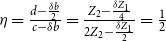 $\eta =\frac {d-\frac {\delta b}{2}}{c-\delta b}=\frac {Z_{2}-\frac {\delta Z_{1}}{4}}{2Z_{2}-\frac {\delta Z_{1}}{2}}=\frac {1}{2}$
for
 $\delta \neq \frac {c}{b}=\frac {4Z_{2}}{Z_{1}}$
.
Moreover, when
 $\delta =0$
, equation (22) reduces to
 \begin{equation*} c\eta -d=0 \end{equation*}
and we have only one interior equilibrium solution
 $\eta _{0}=\frac {d}{c}$
. Consider that
 $d\gt 0$
and recall that
 $0\leq x\leq 1$
, it follows that:
-
1.
$0\lt \eta _{0}\lt 1$
for
$c\gt d$
that holds for
$\theta \lt \overline {\theta }=\frac {2Z_{2}Z_{4}}{x-(1-x)Z_{2}(Z_{3}+Z_{4})}$
if
$\overline {\theta }\gt 0$
that is if
$x\gt \overline {x}=\frac {Z_{2}(Z_{3}+Z_{4})}{1+Z_{2}(Z_{3}+Z_{4})}$
and it holds for any
$\theta \geq 0$
if
$\overline {\theta }\leq 0$
, that is if
$x\leq \overline {x}=\frac {Z_{2}(Z_{3}+Z_{4})}{1+Z_{2}(Z_{3}+Z_{4})}$
;Footnote
18
-
2.
$\eta _{0}\lt 0$
for
$c\lt 0$
, that holds when
$\phi \gt \overline {\phi }=\frac {1}{2\sigma -1}$
(
$Z_{2}Z_{4}\gt \frac {1}{2}$
),
$x\gt \widetilde {x}$
and
$\theta _{1}\lt \theta \lt \theta _{2}$
,where
$\widetilde {x}=\frac {2Z_{2}[2Z_{4}(Z_{2}Z_{3}+1)+Z_{3}(2Z_{2}Z_{3}+1)+2\sqrt {Z_{4}(Z_{3}+Z_{4})(2Z_{2}Z_{3}+1)}]}{[2Z_{2}(Z_{3}+Z_{4}+1)]^{2}},$
$\theta _{1}=\frac {x-[2Z_{2}Z_{3}(1-x)+2Z_{4}Z_{2}(2-x)]-\sqrt {[2Z_{2}(Z_{3}+Z_{4})+1]^{2}x^{2}-4Z_{2}\{Z_{3}[2Z_{2}(Z_{3}+Z_{4})+1]+2Z_{4}\}x+4Z_{2}^{2}Z_{3}^{2}}}{2Z_{2}(1-x)(Z_{3}+Z_{4})},$
$\theta _{2}=\frac {x-[2Z_{2}Z_{3}(1-x)+2Z_{4}Z_{2}(2-x)]+\sqrt {[2Z_{2}(Z_{3}+Z_{4})+1]^{2}x^{2}-4Z_{2}\{Z_{3}[2Z_{2}(Z_{3}+Z_{4})+1]+2Z_{4}\}x+4Z_{2}^{2}Z_{3}^{2}}}{2Z_{2}(1-x)(Z_{3}+Z_{4})},$
-
3.
$\eta _{0}\geq 1$
for
$0\lt c\leq d$
. Where
$c\gt 0$
when
$\phi \leq \overline {\phi }$
(
$Z_{2}Z_{4}\leq \frac {1}{2}$
) or when
$\phi \gt \overline {\phi }$
(
$Z_{2}Z_{4}\gt \frac {1}{2}$
) and
$x\lt \widetilde {x}=\frac {2Z_{2}[2Z_{4}(Z_{2}Z_{3}+1)+Z_{3}(2Z_{2}Z_{3}+1)+2\sqrt {Z_{4}(Z_{3}+Z_{4})(2Z_{2}Z_{3}+1)}]}{[2Z_{2}(Z_{3}+Z_{4}+1)]^{2}}$
,
$\theta \lt \theta _{1}$
and
$\theta \gt \theta _{2}$
; and
$c\leq d$
when
$\theta \geq \overline {\theta }$
, with
$\overline {\theta }\lt \theta _{1}.$




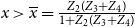


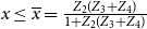





Moreover
 $\frac {d\eta _{0}}{d\theta }\gt 0$
for
 $x\leq \overline {x}$
or for
 $x\gt \overline {x}$
and
 $\frac {d\eta _{0}}{d\theta }\geq (\lt )0$
for
 $\theta \leq (\gt )\widetilde {\theta }=\frac {2Z_{2}Z_{4}(1-x)(Z_{3}Z_{4})+\sqrt {2}\sqrt {[Z_{4}x(1-x)(Z_{3}+Z_{4})(x-Z_{2}Z_{3}(1-x)+Z_{2}Z_{4}(1+x)}}{(1-x)(Z_{3}+Z_{4})[x-(1-x)Z_{2}(Z_{3}+Z_{4})]},$
with
 $\widetilde {\theta }\gt \overline {\theta }.$
Notice that
 $\eta _{0}=0.5$
for
 $\theta =0$
and it is always increasing with
 $\theta$
in the relevant range. From the previous analysis, we derive the following result.
Proposition 2. Let
 $\delta =0$
. The corresponding interior solution
 $\eta =\eta _{0}$
belongs to the interval
 $[0.5,1)$
for
 $0\leq \theta \lt \overline {\theta }$
if
 $\overline {\theta }\gt 0$
and for any
 $\theta \geq 0$
if
 $\overline {\theta }\leq 0.$
It is equal to
 $0.5$
when
 $\theta =0$
and it is increasing in
 $\theta$
.
Considering now the case where
 $\delta \gt 0$
and
 $\theta \gt 0$
, we have that the possible solution for
 $\eta$
associated to the interior equilibria are:
 \begin{eqnarray*} \eta _{1} &=&\frac {\delta b-c-\sqrt {\Delta _{\eta }}}{2\delta a}, \\[6pt] \eta _{2} &=&\frac {\delta b-c+\sqrt {\Delta _{\eta }}}{2\delta a}, \end{eqnarray*}
where
 \begin{equation} \Delta _{\eta }=b(b-2a)\delta ^{2}+2(2ad-bc)\delta +c^{2}. \end{equation}
Since
 $c\lt 2d$
one or two positive solutions for equation (22) may exist. Consider that:
-
a) when
$\frac {c}{b}\leq \delta \lt \frac {2d}{b}$
, we have one positive solution (
$\eta _{2}$
) which is the largest in absolute value; -
b) when
$\delta \geq \frac {2d}{b}$
, we have one positive solution and one non negative solution (
$0\leq \eta _{1}\lt \eta _{2}$
); -
c) when
$\delta \lt \frac {c}{b}$
, we have one positive solution (
$\eta _{2}$
) which is the smallest in absolute value.


Therefore, when it exists (it is real), the solution
 $\eta _{1}$
is positive for any parameter combination in the relevant domain.
To verify the existence of real solutions, we examine the discriminant
 $\Delta _{\eta }$
. Let
 $\Delta _{\delta }=2a[bc(c-2d)+2ad^{2}]$
. We distinguish three cases:
-
Case 1:
$\Delta _{\delta }\lt 0$
. The equation
$\Delta _{\eta }=0$
does not admit real solutions for
$\delta$
. -
Case 2:
$\Delta _{\delta }\gt 0$
. The equation
$\Delta _{\eta }=0$
admits two dinstict solutions for
$\delta$
, given by:with
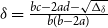
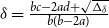
\begin{align*} \delta _{1} & =\frac {bc-2ad-\sqrt {\Delta _{\delta }}}{b(b-2a)},\\[5pt] \delta _{2} & =\frac {bc-2ad+\sqrt {\Delta _{\delta }}}{b(b-2a)}, \end{align*}
$0\lt \delta _{1}\lt \delta _{2}$
for
$c\gt d$
(
$x\lt \overline {x}$
).Footnote
19
-
Case 3:
$\Delta _{\delta }=0.$
The equation
$\Delta _{\eta }=0$
admits a unique solution for
$\delta$
:where the last result is obtained by using the condition
\begin{equation*} \delta =\overline {\delta }=\frac {bc-2ad}{b(b-2a)}=\frac {cd}{b(c-d)}, \end{equation*}
$bc(c-2d)+2ad^{2}=0$
, solved for
$a$
. Moreover,
$\overline {\delta }\gt 0$
as long as
$c\gt d$
.


In Case 1
 $\eta _{1}$
and
 $\eta _{2}$
are always real and distinct. In Case 2 they are real and distinct for
 $\delta \lt \delta _{1}$
and
 $\delta \gt \delta _{2}$
and there is a unique real solution at
 $\delta =\delta _{1}$
or at
 $\delta =\delta _{2}$
, i.e.,
 \begin{equation*}\begin{array} [c]{ccc}\eta =\eta _{a}=\frac {\delta _{1}b-c}{2a\delta _{1}} & \text{at} & \delta =\delta _{1}\\[5pt] \eta =\eta _{b}=\frac {\delta _{2}b-c}{2a\delta _{2}} & \text{at} & \delta =\delta _{2}\end{array} . \end{equation*}
Finally, in Case 3
 $\eta _{1}$
and
 $\eta _{2}$
are real and distinct except at
 $\delta =\overline {\delta }$
where the solution is unique:
 $\eta =\eta _{0}$
.
These results help analyze how parameter
 $\theta$
affects the interior equilibria. Analytical results on
 $\theta$
are difficult to derive, but key conclusions follow. We treat
 $\Delta _{\delta }$
as a function of
 $\theta$
,
 $\Delta _{\delta }=\Delta _{\delta }(\theta ).$
The equation
 $\Delta _{\delta }(\theta )=0$
has up to four solutions:
 $\theta _{1},$
 $\theta _{2},$
 $\theta _{3}$
and
 $\theta _{4}$
. We know
 $\theta _{1}=0$
and
 $\theta _{3}\lt 0$
, while the signs of
 $\theta _{2}$
and
 $\theta _{4}$
depend on parameter values. The sign of
 $\Delta _{\delta }$
never changes if
 $\theta _{2}\lt 0$
and
 $\theta _{4}\lt 0$
, which happens in these two cases:
 \begin{equation*}\begin{array} [c]{ccccc}i) & 0\lt \phi \lt \phi _{\delta } &\quad and & \quad 0\lt x\lt x_{b} & (\Delta _{\delta }(\theta )\text{ always positive}),\\[6pt] ii) & \phi _{\delta }\lt \phi \lt 1 & \quad and & \quad x_{b}\lt x\lt x_{m} & (\Delta _{\delta }(\theta )\text{ always negative}), \end{array} \end{equation*}
with
 $\phi _{\delta }=\frac {1}{2\sigma -1}$
,
 $x_{b}=\frac {1-(\sigma -1)\phi }{\sigma }$
and
 $x_{m}=\frac {(4+\phi )\sigma -(1+\phi )-\sqrt {(\sigma -1)\{[\sigma (\phi ^{2}+8\phi +8)-\phi (2+\phi )]-1\}}}{2\sigma }.$
In other parameter configurations
 $\Delta _{\delta }(\theta )$
may change sign depending on
 $\theta .$
Moreover, in the special cases
 $x=0$
or
 $\phi =\phi _{\delta }$
and
 $x=x_{b}$
,
 $\Delta _{\delta }(\theta )=0$
always.Footnote
20
In our main analysis, we choose
 $\phi _{\delta }\lt \phi \lt 1$
and
 $x_{b}\lt x\lt x_{m}$
corresponding to
 $\Delta _{\delta }(\theta )$
always negative. This ensures
 $\eta _{1}$
and
 $\eta _{2}$
real and distinct for all
 $\theta$
s (notice however that other combinations with
 $\phi \gt \phi _{\delta }$
or
 $x\gt x_{b}$
may yield the same result).
Concerning the behavior of
 $\eta _{1}$
and
 $\eta _{2}$
with respect to
 $\theta$
, we have that when
 $\Delta _{\delta }\lt 0$
and
 $\Delta _{\delta }\gt 0$
(for
 $\Delta _{\delta }\lt 0$
see Figure 3 in the main text where the behavior of
 $\eta _{1}$
is shown) numerical computations show:
-
$\bullet$
at
$\theta =0$
the derivatives are not defined;
-
$\bullet$
when
$\theta$
is approaching
$0$
from the right
$\frac {\partial \eta _{1}}{\partial \theta }\gt 0$
and
$\frac {\partial \eta _{2}}{\partial \theta }\lt 0$
;
-
$\bullet$
for
$\theta$
sufficiently large, as long as
$I_{1}$
and
$I_{2}$
belong to the interior of
$u$
,
$\frac {\partial \eta _{1}}{\partial \theta }\lt 0$
and
$\frac {\partial \eta _{2}}{\partial \theta }\gt 0$
.


Moroever, when
 $\Delta _{\delta }=0,$
 $\eta _{1}$
is monotonically increasing and
 $\eta _{2}$
is monotonically decreasing with respect to
 $\theta$
, with
 $\eta _{1}$
and
 $\eta _{2}$
crossing at some
 $\theta$
 $=\overline {\theta }$
.Footnote
21
Finally, we briefly mention the stability properties of
 $\eta _{1}$
and
 $\eta _{2}$
in correspondence of the three cases mentioned above:
Consider the interior fixed points
 $I_{1}=(\lambda ,\eta _{1})$
and
 $I_{2}=(\lambda ,\eta _{2}),$
located inside the unit square
 $U$
, we have that:Footnote
22
-
1. When Case 1 holds
$I_{1}$
is locally stable, while
$I_{2}$
is always unstable; -
2. When case 2 holds
$I_{1}$
exists and it is locally stable for
$0\leq \theta \lt \theta _{1}$
and
$\theta \gt \theta _{2}$
(with
$\theta _{1}\lt \theta _{2}$
),Footnote
23
while
$I_{2}$
is always unstable. Moreover, when
$\theta =\theta _{1}$
or
$\theta =\theta _{2}$
are crossed, a fold bifurcation is involved;Footnote
24
-
3. When case 3 holds
$I_{1}$
is locally stable (
$I_{2}$
is unstable) for
$0\leq \theta$
$\lt \overline {\theta }$
and
$I_{2}$
is locally stable (
$I_{1}$
is unstable) for
$\theta$
$\gt \overline {\theta }$
, where local stability is lost and gained via a transcritical bifurcation at
$\theta$
$=\overline {\theta }$
.


This numerical analysis confirms robustness of our result (that is, it holds for a large set of parameters) according to which for
 $\theta$
sufficiently close to
 $0$
, an increase of this parameter determines a rise of the share of capital located in Region 1 (
 $\eta )$
, while by increasing further
 $\theta$
sooner or later this share decreases. This occurs along
 $I_{1}$
when
 $\Delta _{\delta }\lt 0$
and
 $\Delta _{\delta }\gt 0$
(admitting for a range of values of
 $\theta$
—i.e.
 $\theta _{1}\lt \theta \lt \theta _{2}$
—for which
 $I_{1}$
does not exist if
 $\Delta _{\delta }\gt 0$
) and along
 $I_{1}$
for
 $0\leq \theta$
 $\lt \overline {\theta }$
and along
 $I_{2}$
for
 $\theta \gt \overline {\theta }$
when
 $\Delta _{\delta }=0$
.
A.3 Border Equilibria
Border equilibria are defined as points on the boundary of
 $U$
excluding its corners.
Border fixed points belonging to the interior of the horizontal side of
 $U$
, are:
 $B$
and
 $B''\in \{(\lambda ,\eta ) \, : \, 0\lt \lambda \lt 1,\eta =0\}$
, and
 $B'$
and
 $B'''\in \{(\lambda ,\eta )\, : \, 0\lt \lambda \lt 1,\eta =1\}.$
The coordinates
 $\lambda$
of fixed points lying on the lower horizontal border of
 $U$
are solutions (when they exist and are feasible) of the following equations:
 \begin{equation*} -\delta A_{0}\lambda ^{2}+\delta B_{0}\lambda +C_{0}-\frac {\delta }{4}\frac {B_{0}^{2}}{A_{0}}=0, \end{equation*}
where
 \begin{align*} A_{0} &= \frac {H^2\alpha ^{2}(1-\phi )^{2}E^{2}}{2F^2} \gt 0, \\[5pt] B_{0} &= \frac {EH^2\alpha ^{2}(1-\phi )(2E+L+\phi L)}{2F^2} \gt 0, \\[5pt] C_{0} &= \alpha \frac {(1-\phi )}{\sigma - 1} \frac {H}{F} \gt 0, \end{align*}
with
 $B_{0}\gt 2A_{0}.$
When
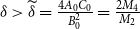 $\delta \gt \widetilde {\delta }=\frac {4A_{0}C_{0}}{B_{0}^{2}}=\frac {2M_{4}}{M_{2}}$
both solutions are positive; while one is positive and one is negative for
 $\delta \lt \widetilde {\delta }$
. The solutions are:
 \begin{eqnarray*} \lambda _{1}^{B0} &=&\frac {\delta B_{0}-\sqrt {4\delta A_{0}C_{0}}}{2\delta A_{0}}, \\[5pt] \lambda _{2}^{B0} &=&\frac {\delta B_{0}+\sqrt {4\delta A_{0}C_{0}}}{2\delta A_{0}}. \end{eqnarray*}
We have that
 $0\lt \lambda _{1}^{B0}\lt 1$
for
 $\widetilde {\delta }\lt \delta \lt \overline {\delta }=\frac {4A_{0}C_{0}}{(B_{0}-2A_{0})},$
while
 $\lambda _{2}^{B0}\gt 1$
always.
The coordinates
 $\lambda$
of fixed points lying on the upper horizontal side of
 $U$
, are solutions (when they exist and are feasible) of the following equation:
 \begin{equation*} \delta A_{1}\lambda ^{3}+\delta B_{1}\lambda ^{2}+(\delta C_{1}-D_{1})\lambda +\delta E_{1}-F_{1}, \end{equation*}
where
 $A_{1}=8\alpha ^{2}E^{3}H\sigma (\sigma -1)(1-\phi )^{2}[1+\theta (1-x)]\gt 0,$
 $B_{1}=4\alpha ^{2}E^{2}H\sigma (\sigma -1)(1-\phi )[1+\theta (1-x)][L(3+\phi )+4E\phi ]\gt 0,$
 $C_{1}=2\alpha ^{2}EH\sigma (\sigma -1)[1+\theta (1-x)][L(1+\phi )+2E\phi ][L(3-\phi )+2E\phi ]\gt 0,$
 $D_{1}=16\alpha EF(1+\theta )^{3}(1-\phi )[\sigma -\theta (\sigma -x(2\sigma -1))]\geq (\lt )0,$
 $E_{1}=\alpha ^{2}LH\sigma (\sigma -1)[1+\theta (1-x)][L(1+\phi )+2E\phi ]^{2}\gt 0,$
 $F_{1}=8\alpha F(1+\theta )^{3}[\sigma L(1-\phi )(1+\theta )-x\theta \lbrack L(2\sigma -1-\phi )+2E\phi (\sigma -1)]]\geq ({\lt})0.$
Depending on parameter values, we can have at most two positive real roots (that may both lie within the unit interval). Given the parameter constellation considered in the paper, only one positive root is possible,
 $\lambda ^{B_{1}}$
, with
 $0\lt \lambda ^{B_{1}}\lt 1$
for some range of theta values within the interval [0, 0.5].
Finally, as mentioned in the main text, vertical borders are not possible because of the definition in equation (20).