Nomenclature
- A
-
area (m2)
- Cx
-
drag coefficient
- H
-
specific enthalpy (J/kg)
- m
-
mass flow rate (kg/s)
- Ma
-
Mach number
- P
-
static pressure (Pa)
- Pt
-
total pressure (Pa)
- R
-
gas constant (J/(mol·K)
- T
-
static temperature (K)
- Tt
-
total temperature (K)
- V
-
velocity (m/s)
Greek symbol
-
 $ \beta$
-
boundary layer thickness (m)
-
$ \gamma$
-
specific heat ratio
-
$ \delta$
-
total deflection angle (deg)
-
$ \varepsilon$
-
residual error
-
$ \theta$
-
shock wave angle (deg)
-
$ \rho$
-
density (kg/m3)
-
$ \sigma$
-
total pressure recovery coefficient
-
$ \varphi$
-
flow coefficient


Abbreviation
- AUSM
-
advection upstream splitting method
- CFD
-
computational fluid dynamics
- CR
-
contraction ratio
- TBCC
-
turbine-based combined cycle
Subscripts
- 0
-
freestream
- ave
-
average
- BL
-
boundary layer
- core
-
core flow
- in
-
inlet entrance
- out
-
inlet exit
- t
-
throat
1.0 Introduction
Facing the demand for aerospace integration, hypersonic vehicles have become a primary development direction for future aircraft, attracting worldwide attention and driving intense global research efforts [Reference Bertin and Cummings1–Reference Ma, Zhang and Liu3]. The flight range spans subsonic, supersonic and hypersonic regimes, with high-performance propulsion systems being critical for achieving hypersonic flight. Air-breathing scramjet engines, which extract oxygen directly from the atmosphere without carrying oxidisers, significantly reduce vehicle weight and enhance specific impulse, making them the preferred propulsion system for hypersonic vehicles [Reference Das, Pandey and Sharma4]. The hypersonic inlet is a critical component of scramjet or combined-cycle engines, tasked with capturing and compressing freestream airflow to ensure high-quality flow delivery to the combustion chamber. Its efficient operation directly impacts propulsion performance and aircraft capabilities. A key requirement for inlet functionality is self-starting capability, which fails at low Mach numbers when the captured flow rate exceeds the inlet’s flow capacity. To ensure that the inlet can keep self-starting at low Mach numbers, the contraction ratio (CR) can’t be too large, while to ensure the excellent performance of the inlet at high Mach numbers, the CR can’t be too small [Reference Van Wie, Kwok and Walsh5]. Currently, a relatively effective solution is to change the geometry of the inlet under different inflow conditions, which can make the inlet self-starting at low Mach numbers and meet the performance requirements at high Mach numbers. Therefore, the variable-geometry inlet has become the preferred choice for the wide-speed-range engine or combined engine.
The design of the internal flow surface of a variable-geometry inlet is of paramount importance, as it directly affects the performance of the inlet. Currently, a lot of scholars have conducted relevant research, mainly focusing on the variable geometry design of the compression ramp and cowl [Reference Liu, Shi, Liu, Qin and He6–Reference Wang, Yuan, Zhang and Zhou13]. In terms of rotating the compression ramp, Liu et al. [Reference Liu, Shi, Liu, Qin and He6] designed a wide-range variable geometry inlet through the rotation of the ramp, completing a transition between single and dual flow paths. The inlet achieves comprehensive high-mass capture coefficients in the overall wide flight range, especially in a low-speed stage. Yuan et al. [Reference Yuan, Liu, Zhang and Wang7] also designed a variable geometry inlet by rotating ramps. The results from the numerical simulations and experimental tests indicated that the designed inlet could work properly during this Mach number range. The mass flow captured by the inlet and total pressure recovery at turbine/ramjet aerodynamic interface planes met the requirements of the Turbine-Based Combined Cycle (TBCC) propulsion system. In terms of changing the cowl, Teng et al. [Reference Teng and Yuan8] used a variable geometry cowl sidewall control technique in a generic rectangular hypersonic inlet, in an effort to improve inlet performance under both on-design and off-design conditions. The research results show that the increased cowl sidewall sweepback expands the inlet flow spillage window, thus effectively restarting the inlet from an unstart status. Wu et al. [Reference Wu, Wang, Quan and Chang9] adopted the design concept of a variable-geometry inlet scheme that combines the variable-geometry cowl with regulating shock wave elimination. The results demonstrate that the variable-geometry inlet featuring a translatable and rotatable cowl can effectively control, and in some cases completely suppress, flow separation phenomena. Furthermore, Yuan et al. [Reference Yuan and Guo10] designed a variable geometry inlet through rotating and horizontally moving the cowl, and found that the aerodynamic performance of the variable geometry inlet was significantly better than that of the fixed geometry inlet at low Mach numbers.
The variable geometry inlet with changing the position of the cowl and ramp had better performance in the entire operating range. However, most of the above designs are based on the inviscid assumption, which often results in a flow coefficient of less than 1.0 at the design point, and the characteristic laws of variable geometry have not been provided in detail. In general, the complete design process of a variable geometry inlet should be divided into two stages – one is the design point geometry design, and the other is the off-design point geometry design. As the benchmark of off-design point variable geometry design, the design point geometry affects the performance of the whole inlet and needs to be designed emphatically. Moreover, most studies are based on numerical simulation or experiment, which will consume a lot of time and prolong the design cycle of variable geometry inlets. By comparison, the one-dimensional model simplifies the fluid flow process in the inlet with some mathematical models, and the calculation speed is fast, which is suitable for the initial design of the inlet [Reference Gopal and Wilson14–Reference Kopasakis, Connolly and Kratz18]. Gopal et al. [Reference Gopal and Wilson14] used a one-dimensional model to analyse a typical scramjet inlet operation at on-design and off-design conditions. Moreover, a comprehensive validation of the one-dimensional model was conducted through experimental and computational data. Dalle et al. [Reference Dalle, Fotia and Driscoll15] proposed a one-dimensional model to predict a steady two-dimensional supersonic flow through an inlet. The results were compared to experimental data, and the model inaccuracies were found to be limited to 10%. A comparison with computational fluid dynamics (CFD) showed that the averaged thermodynamic properties at the exit of a scramjet inlet could be estimated, and the proposed model could be used in a control-oriented model of a scramjet vehicle. Additionally, Dalle et al. [Reference Dalle, Torrez and Driscoll16] also adopt the one-dimensional model to improve inlet performance by using a variable-geometry cowl.
While one-dimensional models have been successfully applied to inlet design and performance evaluation, their modeling methodologies still suffer from inherent limitations in terms of completeness. Especially for the mixing problem of the boundary layer flow and core flow at the inlet exit, there is still a lack of models that consider the influence of the boundary layer. In the face of practical research status and application demands, this paper proposes a design method based on the one-dimensional model for a variable-geometry inlet. In the design point stage, the proposed method takes into account the effects of the boundary layer and modifies the initial design geometry to bring the external compression shock wave to the cowl lip. In the variable geometry design stage, geometric variations are done through the ramp rotation and horizontal movement of the cowl, ensuring the inlet is self-starting at the low Mach numbers and maintains the optimal performance in a wide speed range.
2.0 Description of design method and models
2.1 Two-dimensional variable geometry inlet
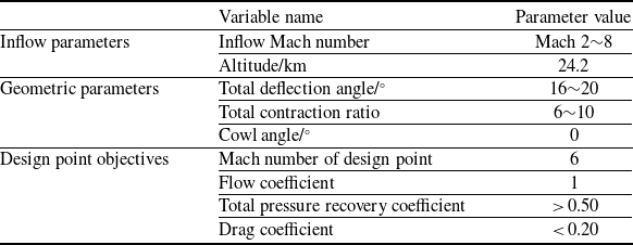
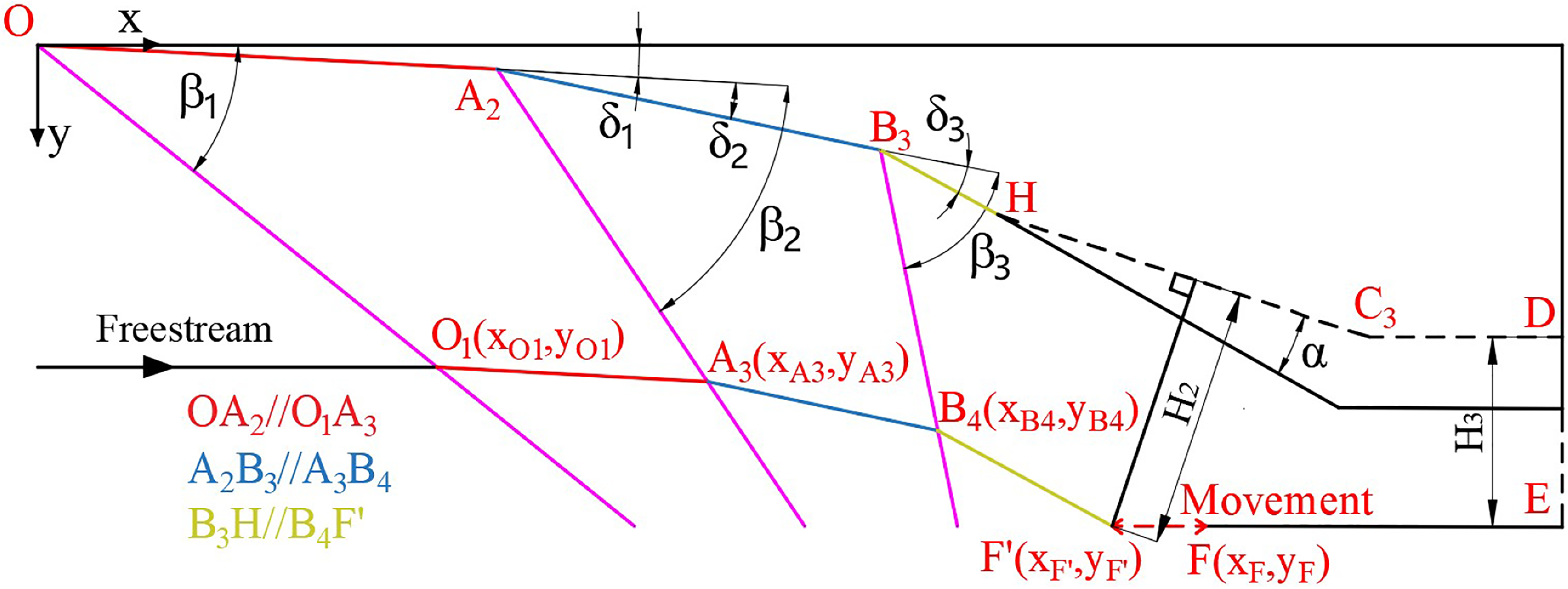
At present, the common hypersonic inlets mainly include two-dimensional inlets, axisymmetric inlets, three-dimensional inward-turning inlets and so on [Reference Abedi, Askari, Sepahi-Younsi and Soltani19, Reference Wang, Tian, Deng and Wang20]. Among them, the two-dimensional inlet has advantages such as wide-range adaptability, convenience for large-scale modularisation and geometric adjustment, which has potential application value in aerospace integrated propulsion systems for a wide speed range. The paper utilises the model analysis method to design a two-dimensional variable geometry inlet. The design scheme selects a mixed compression inlet with three external compression shock waves and one internal compression shock wave. The inlet schematic is presented in Fig. 1, with its design parameters summarised in Table 1. As shown in the figure, each ramp of the inlet causes the inflow to deflect and generate the oblique shock wave. In the ideal design state, the three external compression waves intersect at the cowl lip, and the cowl-lip shock wave intersects at the shoulder point, which can obtain relatively ideal fluid performance parameters. However, under off-design point conditions, performance parameters may sharply decline, which is why the variable geometry design is necessary.
Design parameters of the two-dimensional inlet

Table 1. Long description
A table with three columns and eight rows, detailing the design parameters of a two-dimensional inlet. The columns are labeled Variable name, Parameter value, and include inflow parameters, geometric parameters, and design point objectives. Row 1: Inflow parameters, Inflow Mach number, Mach 28. Row 2: Inflow parameters, Altitude/km, 24.2. Row 3: Geometric parameters, Total deflection angle/, 1620. Row 4: Geometric parameters, Total contraction ratio, 610. Row 5: Geometric parameters, Cowl angle/, 0. Row 6: Design point objectives, Mach number of design point, 6. Row 7: Design point objectives, Flow coefficient, 1. Row 8: Design point objectives, Total pressure recovery coefficient, > 0.50. Row 9: Design point objectives, Drag coefficient, < 0.20.
Schematic diagram of the two-dimensional variable geometry inlet.

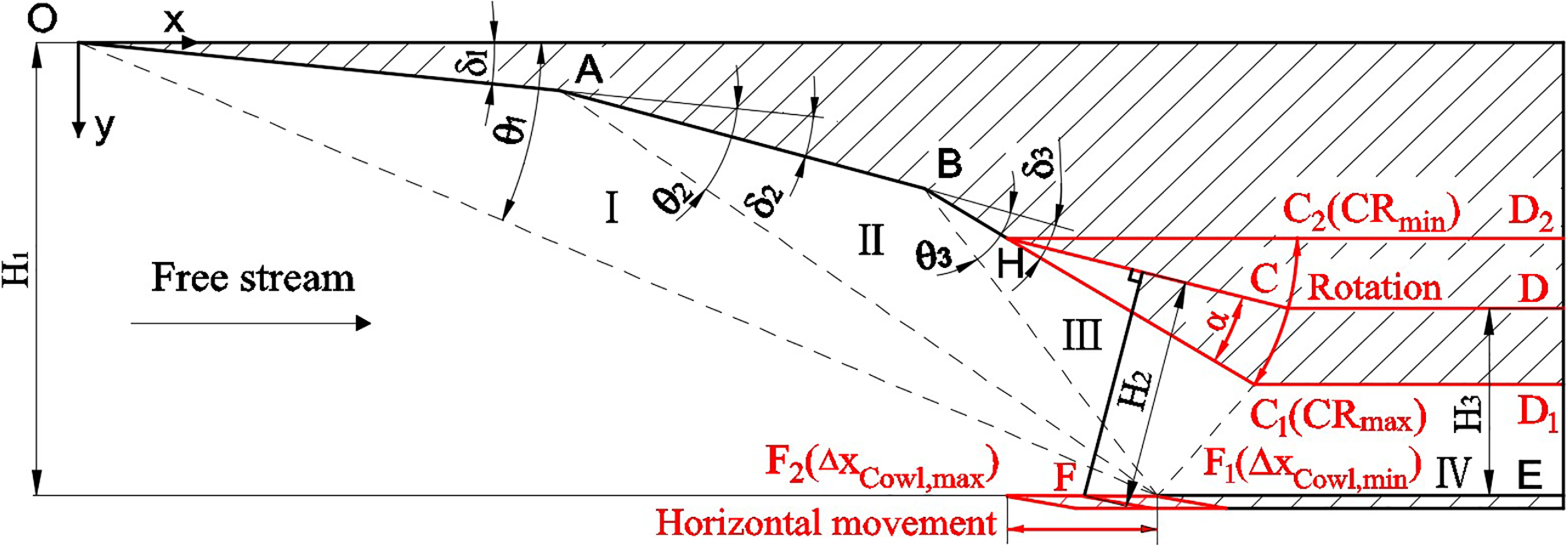
The two-dimensional variable geometry inlet studied in this paper includes two kinds of variable geometry, namely throat height adjustment and cowl-lip translation adjustment. The adjustment methods are described as follows: a rotation point H is set on the last compression ramp. The movable compression ramp and the flat throat plate are rotated around the rotation point H to achieve the purpose of throat height adjustment, meeting the CR requirements under the different Mach number conditions.
Among them, the total CR is defined as the ratio of the inlet capture height H 1 to the throat height H 3 and the expression is given in Equation (1). The CRmax and CRmin represent the upper and lower limits of the CR in Fig. 1.
 \begin{align} \text{CR}=\frac{{H}_{1}}{{H}_{\text{3}}}\text{}\end{align}
Meanwhile, the cowl lip of the inlet can be adjusted for a forward or backward translation, allowing for controlling the proportion of captured airflow based on the distribution of external compression shock waves under different Mach number conditions. Among them, the translation distance of the cowl lip is defined as the difference between the design point x-coordinate x
Design of the cowl lip and the actual x-coordinate x
F of the cowl lip, and the expression is given in Equation (2). If the
 $ \Delta {x}_{Cowl}$
is a positive value, it indicates a movement to the left from the design point. If it is a negative value, it indicates a movement to the right from the design point. The
 $ \Delta {x}_{Cowl,\mathrm{max}}$
and
 $ \Delta {x}_{Cowl,\mathrm{min}}$
are represent the upper and lower limits of cowl-lip movement. In order to carry out dimensionless processing, the relative movement distance
 $ \Delta {\overline{x}}_{Cowl}$
is defined in Equation (3).
 \begin{align} \Delta {x}_{Cowl}={x}_{Design}\text{-}x{}_{F}\end{align}
 \begin{align} \Delta {\overline{x}}_{Cowl}=\frac{\Delta {x}_{Cowl}}{\Delta {x}_{Cowl,\mathrm{max}}-\text{}\Delta {x}_{Cowl,\mathrm{min}}}\end{align}
The combination adjustment of throat height and cowl-lip translation will change the internal CR of the inlet, thereby affecting the starting capability of the inlet. Therefore, the boundary constraint requirement is to ensure that the inlet is in a start-up state at each Mach number. Among them, the internal CR is defined in Equation (4).
 \begin{align} {\text{CR}}_{\text{internal}}=\frac{{H}_{2}(\text{CR},\Delta {x}_{cowl})}{{H}_{3}}\end{align}
Similar to traditional inlets, the main objectives of variable geometry inlets are the flow coefficient, total pressure recovery coefficient, throat Mach number, drag coefficient and starting performance. In theory, by adjusting the variable geometry of the inlet, it is possible to achieve high flow capture efficiency and compression performance within a wide Mach number range, while ensuring the starting ability of the inlet.
2.2 Design method
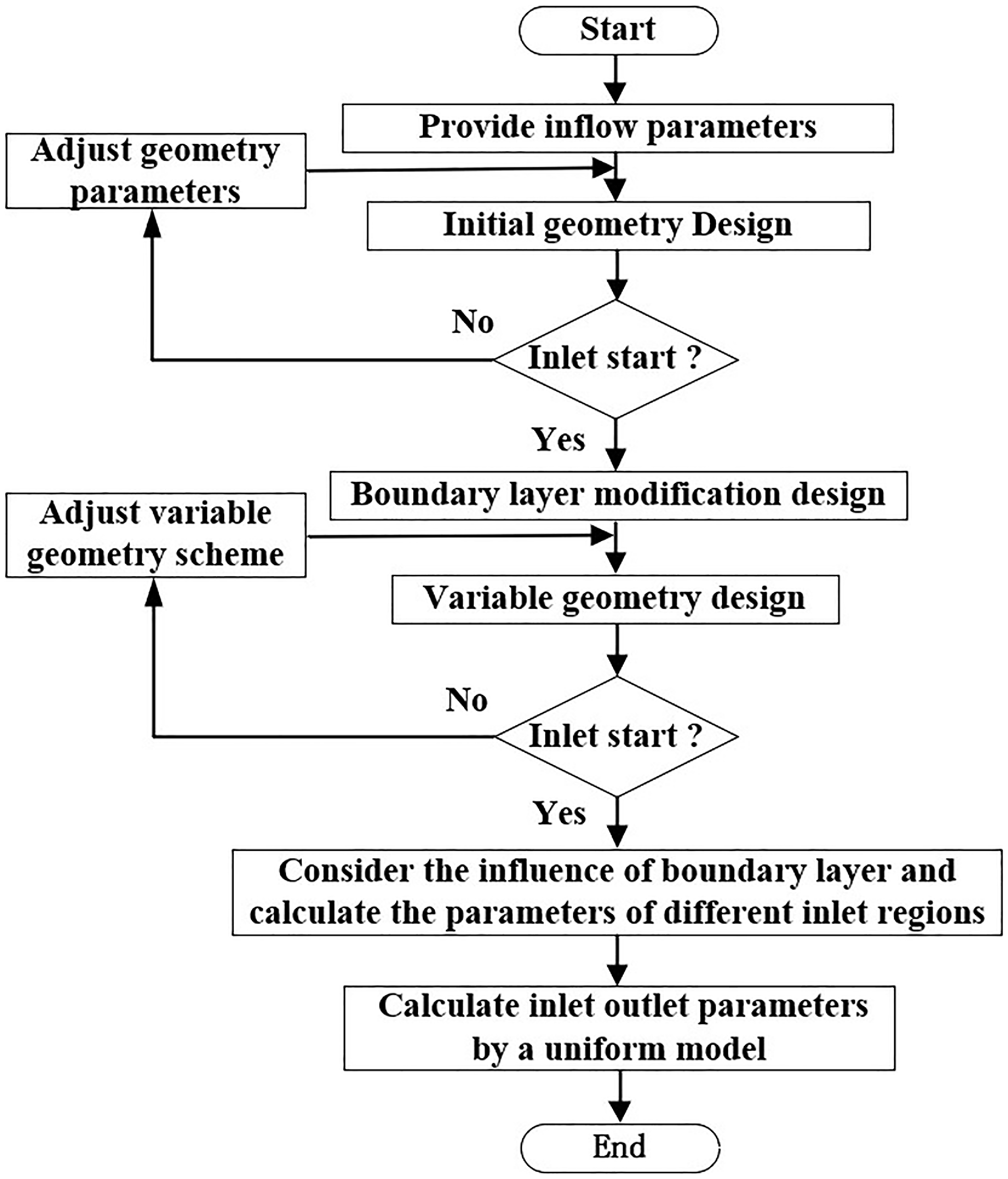
The simplified design process of variable geometry inlet is shown in Fig. 2, which includes the initial geometric design, boundary layer correction design and variable geometry design.
Design process of the variable geometry inlet.

2.2.1 Initial geometric design under design-point condition
When designing the inlet, the two design parameters are very important, namely the deflection angle (
 $ \delta$
) and CR. To choose two parameters, a wide design range is first given in Table 1. Based on the equal shock intensity design method [Reference Huo, Yang, Zhang and Liu21], the multiple sets of performance parameters can be obtained by using different
 $ \delta$
and CR, and then the
 $ \delta$
and CR meeting the design requirements can be selected as the final design parameters. The design process of equal shock intensity is given as follows. As shown in Fig. 1, the initial value of the first deflection angle
 $ \delta$
1 is given, and the first oblique shock angle
 $ \theta$
1 and gas parameters in zone I are obtained by using the oblique shock calculation model. Based on the equal shock intensity Equation (5), the second oblique shock angle
 $ \theta$
2 and gas parameters in zone II can be calculated. Similarly, the third oblique shock angle
 $ \theta$
3 and gas parameters in zone III can also be obtained.
 \begin{align} M{a}_{0}\,\mathrm{sin}\,{\theta }_{1}=M{a}_{1}\,\mathrm{sin}\,{\theta }_{2}=M{a}_{2}\,\mathrm{sin}\,{\theta }_{3} \\[-10pt] \nonumber\end{align}
At this point, the second and third deflection angles
 $ \delta$
2 and
 $ \delta$
3 can be determined based on the second and third oblique shock angles and parameters before and after the oblique shock wave. With the given
 $ \delta$
, the first deflection angle
 $ \delta$
1 of the next iteration is updated. The above calculations are repeated iteratively to update the three deflection angles
 $ \delta$
1,
 $ \delta$
2 and
 $ \delta$
3 until the desired accuracy
 $ \varepsilon$
is satisfied.
 \begin{align} \left|\delta -({\delta }_{1}+{\delta }_{2}+{\delta }_{3})\right|\le \varepsilon \end{align}
After determining the three deflection angles
 $ \delta$
1,
 $ \delta$
2 and
 $ \delta$
3, the fourth deflection angle
 $ \delta$
4 can be obtained based on the given
 $ \delta$
using geometric relationships. The downstream parameters of the fourth shock wave are also calculated using the oblique shock model.
 \begin{align} {\delta }_{4}={\delta }_{1}+{\delta }_{2}+{\delta }_{3}\end{align}
The calculation method for the fourth shock wave is consistent with that of the previous oblique shock wave calculation. So far, all compression ramp angles, shock angles and downstream parameters of the oblique shock wave have been determined.
2.2.2 Boundary layer modification design
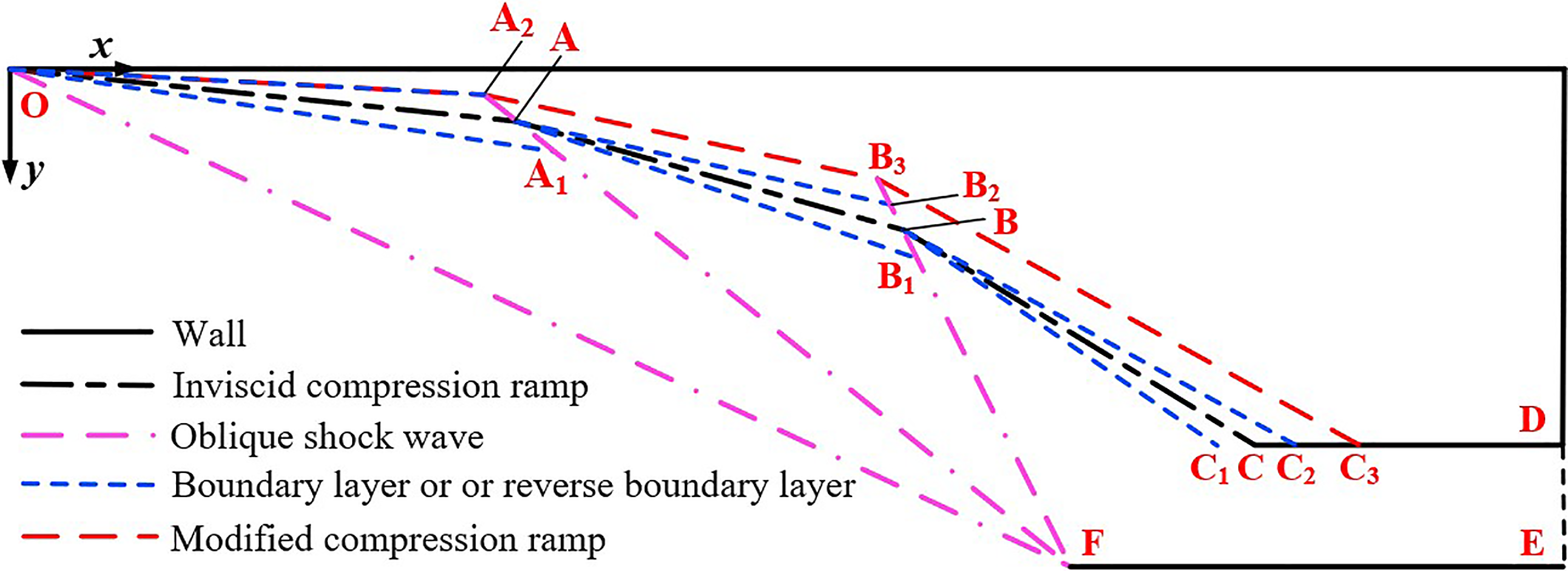
The initial design of the inlet based on the inviscid assumption can cause the shock wave to intersect at the cowl lip, but considering the influence of viscosity can cause the shock wave to deviate from the cowl lip. To ensure that the three external compression shock waves still intersect at the cowl lip when considering the boundary layer, modifications of the inlet geometry are required. The specific modified approach involves first using the boundary layer calculation to get the thickness of the boundary layer, and then subtracting the corresponding boundary layer thickness from the original ramp height to obtain the value as the modified ramp height. The modified ramp, composed of the red line OA 2, A 2 B 3 and B 3 C 3, as shown in Fig. 3, is converted from the inviscid compression ramp composed of the black line OA, AB and BC.
Schematic diagram of inlet design using boundary layer modification.

First, the thickness of the boundary layer along line OA can be determined according to the inflow conditions, so that the equivalent blue line OA 1 after considering the boundary layer can be obtained, and then the shock wave line OO 1 and the parameters behind the shock wave can be obtained by using the oblique shock wave calculation. Afterward, further reverse modification can obtain line OA 2 as the first ramp, which is obtained by the symmetry of line OA 1 with respect to line OA. Next, the airflow behind the first shock wave is taken as the initial inflow, and the boundary layer profile AB 1 and shock wave line AA 3 can also be obtained. The coordinates of the intersection point A 2 can be determined by combining the straight line AA 3 and the straight line OA 2. According to the symmetry relationship, line AB 2 is obtained by the symmetry of line AB 1 with respect to line AB. So, line A 2 B 3 is equivalent to the modified second ramp, which passes through point A 2 and has a slope of line AB 2. By combining lines A 2 B 3 and B 3 B 4, the coordinates of the intersection point B 3 can be determined. Similarly, the modified third ramp can be obtained. After modification, all three external compression oblique shock waves intersect at the lip of the cowl at the design point state, and the inlet operates at the rated state, which can effectively improve the performance of the inlet.
2.2.3 Variable geometry design
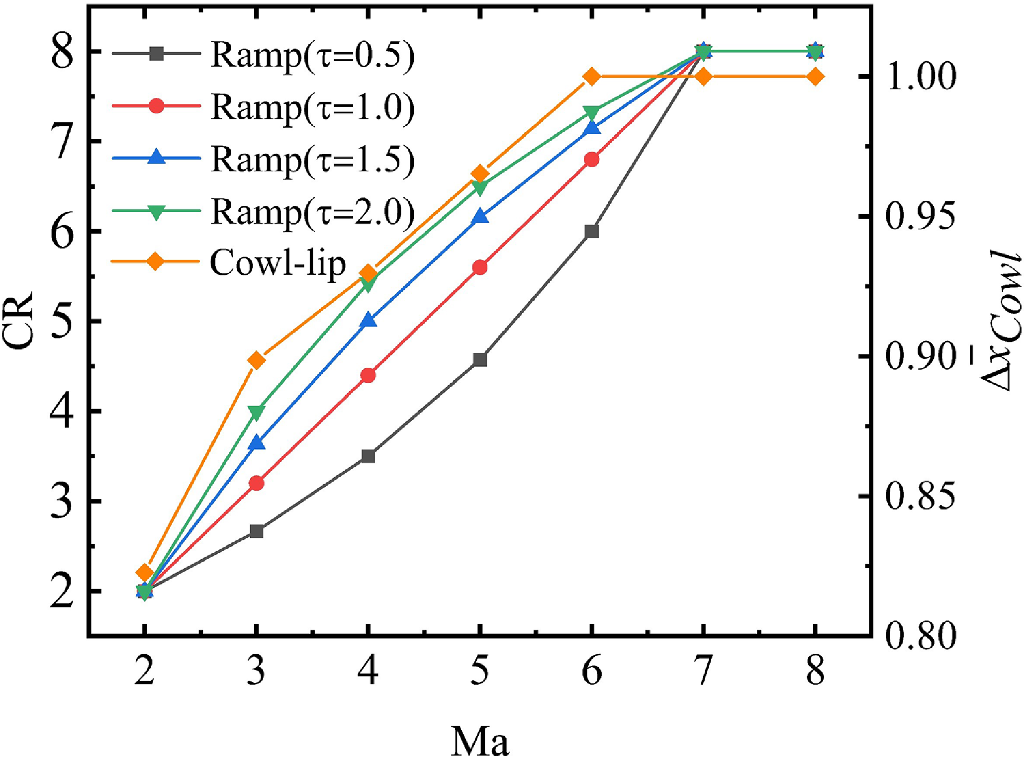
To achieve a self-starting ability and good inlet performance in the wide speed range, changing inlet geometry is a good choice. Based on the geometry of the design point modified by the boundary layer modification, the final compression ramp and the flat throat plate are adjusted to change throat height under different inflow conditions; at the same time, the cowl also moves with the inflow Mach number. In order to ensure that the change of CR does not affect the flow coefficient, the rotation point H is not set at the starting point of the final compression ramp. The x-coordinate of rotation point H is set to be consistent with the x-coordinate of the leftmost movement position of the cowl-lip. This is because the leftmost movement of the cowl lip can occur under the condition of the minimum inflow Mach number; at that time, the rotating ramp and throat plate are also maintained horizontally. If the x-coordinate of rotation point H is consistent with the x-coordinate of the cowl lip, it can transform the mixed compression inlet into an external compression inlet, effectively improving the starting capability of the inlet. The adjustment scheme for the cowl is to move horizontally along the x-axis with the change of Mach number, and the specific position at each Mach number is determined by the given flow coefficient. It remains unchanged after the Mach number is greater than 6. The relationship between the Mach number and flow coefficient is given based on design experience, as shown in Table 2.
Flow coefficient under different inflow Mach number

Table 2. Long description
A table titled Flow coefficient under different inflow Mach number presents the relationship between Mach number and flow coefficient. The table has two columns and eight rows, including the header row. The first column is labeled Mach number and the second column is labeled Flow coefficient. The values in the table are as follows: Row 1: Mach number, 2, 3, 4, 5, 6, 7, 8. Row 2: Flow coefficient, 0.65, 0.75, 0.84, 0.92, 1, 1, 1. The table shows that the flow coefficient increases with the Mach number up to a value of 6, after which it remains constant at 1.
The corresponding flow coefficient
 $ \varphi$
(Ma) can be obtained for a known inflow condition in Table 2, and then the position of the cowl lip can be determined based on the geometric relationship shown in Fig. 4. Because the known
 $ \varphi$
is equivalent to giving the y-coordinate y
O1
of point O
1, and the deflection angles and shock angles of different regions are also known, so the coordinates of points O
1, A
3, B
4 and F
′ can be obtained sequentially by the geometry relationship. Therefore, the relative movement distance
 $ \Delta {\bar{x}}_{Cowl}$
can also be expressed as follows.
 \begin{align} \Delta {\overline{x}}_{Cowl}(Ma)=\frac{{x}_{Design}-{x}_{F}(\varphi (Ma))}{\Delta {x}_{Cowl,\mathrm{max}}-\text{}\Delta {x}_{Cowl,\mathrm{min}}}\text{}(M{a}_{\mathrm{min}}\lt Ma\lt M{a}_{\mathrm{max}})\end{align}
Geometric relationship between cowl-lip coordinate and flow coefficient.

After determining the movement pattern of the cowl and the rotation point H,
 $ \tau$
function of CR is used for control for Mach numbers in the range of 2∼7. While for Mach numbers in the range of 7∼8, the constant CR is used for control. The equation for the control rule of
 $ \tau$
function is given by Equation (9).
 \begin{align} \begin{cases}\text{CR} (Ma)={\text{CR}}_{\mathrm{min}}+\dfrac{({\text{CR}}_{\mathrm{max}}-{\text{CR}}_{\mathrm{min}})\cdot \tau \cdot a}{1+(\tau -1)\cdot a} &M{a}_{\mathrm{min}}\le Ma\le M{a}_{tran}\\[15pt] \text{CR} (Ma)={\text{CR}}_{\mathrm{max}} &M{a}_{tran}\le Ma\le M{a}_{\mathrm{max}}\end{cases} \end{align}
Where Ma is the inflow Mach number, Ma
min
and Ma
max
are the input minimum and maximum Mach numbers, Ma
tran
is the transition Mach number of the
 $ \tau$
function and the constant value equation, CR
min
and CR
max are the input minimum and maximum CRs and
 $ \tau$
is the input control parameter. Additionally, a represents the relative value of the inflow Mach number within the input Mach number range shown in Equation (10).
 \begin{align} a=\frac{Ma-M{a}_{\mathrm{min}}}{M{a}_{\mathrm{max}}-M{a}_{\mathrm{min}}}\end{align}
Therefore, it is easy to calculate the rotation angle
 $ \alpha$
under the condition of the given CR, the expression is displayed in Equation (11).
 \begin{align} \alpha =\delta \text{-}\mathrm{arcsin}\! \left(\frac{{y}_{{C}_{3}}-{y}_{H}}{{L}_{H{C}_{3}}} \right)\end{align}
Where y
H
is the y-coordinate of point H,
 $ {y}_{{C}_{3}}$
is the y-coordinate of point C
3,
 $ {L}_{H{C}_{3}}$
is the length of the rotation ramp, and
 $ \delta$
is the total deflection angle. After the known rotation angle
 $ \alpha$
, the expression of CR
internal
can be obtained in Equation (12).
 \begin{align} {\text{CR}}_{internal}=\frac{\left|\mathrm{tan}(\delta -\alpha )({x}_{F}-{x}_{H})+{y}_{F}-{y}_{H}\right|}{\sqrt{{\mathrm{tan}}^{2}(\delta -\alpha )+1}\cdot {H}_{3}}\end{align}
Where x F and y F are the x-coordinate and y-coordinate of point F, x H and y H is x-coordinate and y-coordinate of point H, and H 3 is the throat height. Finally, the specific adjustment scheme for the rotation of the final ramp and movement of the cowl lip is shown in Fig. 5.
The specific adjustment scheme of the final ramp and cowl lip.

2.3 Design models
To simplify the design process of inlets via the one-dimensional model method, the following foundational assumptions are established. Firstly, the inflow is assumed to behave as an ideal gas, in full compliance with fundamental thermodynamic laws; secondly, the inflow field remains spatially and temporally uniform at all stages; thirdly, the fluid inside the inlet does not undergo any heat exchange with the external environment. The main models utilised in the design process are displayed as follows.
2.3.1 Oblique shock wave model
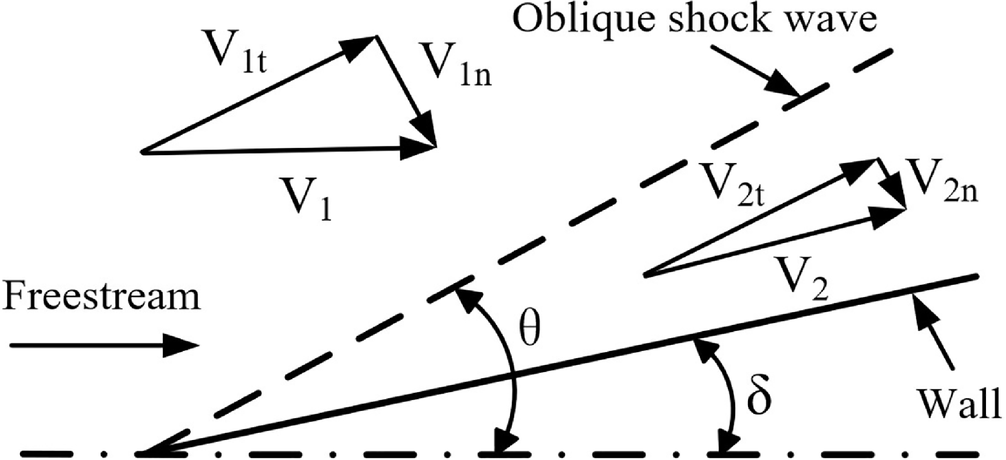
The flow process of supersonic inflow in the inlet can be equivalent to a multi-shock compression process, and oblique shock waves are generated by the external compression ramp during the stable operation of the inlet, as shown in Fig. 6. Normal shock waves or bow shock waves are unstable in the external compression ramp and can cause the inlet to unstart. In order to ensure the stable operation of the inlet, the shock waves should be configured when designing the compression ramp of the inlet. If the Mach number of the supersonic inflow is large, the calculation of the oblique shock wave needs to consider the variation of the
 $ \gamma$
[Reference Burcat and Ruscic22]. The calculation process of oblique shock waves is given below. According to the compression characteristics of the oblique shock wave, the tangential velocity component along the shock wave remains unchanged.
 \begin{align} {V}_{1t}={V}_{2t}\end{align}
Schematic diagram of oblique shock wave.

The normal velocity component along the shock wave satisfies the following relation.
 \begin{align} \frac{{V}_{2n}}{{V}_{1n}}=\frac{\mathrm{tan}(\theta -\delta )}{\mathrm{tan}\kern1pt\theta }\end{align}
At the same time, the parameters before and after the shock wave satisfy the state Equation (15), flow conservation Equation (16), momentum conservation Equation (17) and energy conservation Equation (18).
 \begin{align} P=\rho RT \\[-10pt] \nonumber \end{align}
 \begin{align} {\rho }_{1}{V}_{1n}={\rho }_{2}{V}_{2n} \end{align}
 \begin{align} {P}_{1}-{P}_{2}={\rho }_{2}{V}_{2n}^{2}-{\rho }_{1}{V}_{1n}^{2} \\[-10pt] \nonumber \end{align}
 \begin{align} {H}_{1}+\frac{{V}_{1n}^{2}}{2}={H}_{2}+\frac{{V}_{2n}^{2}}{2}\\[10pt] \nonumber \end{align}
Assuming that x and y are expressed as follows.
 \begin{align} \left \{ \begin{array}{c}x={\gamma }_{1}M{a}_{1n}^{2}\\[5pt] y={\gamma }_{2}M{a}_{2n}^{2}\end{array} \right.\end{align}
where
 $ \gamma$
1
and
 $ \gamma$
2
are the specific heat ratios before and after the shock wave, which are not equal after considering the variable
 $ \gamma$
. Ma
1n
and Ma
2n
are the normal Mach numbers before and after the shock wave. From the flow conservation Equation (16) and momentum conservation Equation (17), the following relationship can be obtained by using the ideal gas state equation and the sonic equation.
 \begin{align} y =\frac{1}{\left(\dfrac{1+x}{x}\right)\dfrac{{\rho }_{2}}{{\rho }_{1}}-1}\end{align}
The expressions for the temperature rise ratio, pressure rise ratio and the conservation of energy equation before and after the shock wave can be further derived as follows.
 \begin{align} \frac{{P}_{2}}{{P}_{1}} &=\frac{1+x}{1+y} \\[-10pt] \nonumber \end{align}
 \begin{align} \frac{{T}_{2}}{{T}_{1}}&=\frac{{P}_{2}}{{P}_{1}}\frac{{\rho }_{1}}{{\rho }_{2}} \\[-10pt] \nonumber \end{align}
 \begin{align} H\!\left({T}_{1}\right)+\frac{xR{T}_{1}}{2} &=H\!\left({T}_{2}\right)+\frac{yR{T}_{2}}{2} \\[10pt] \nonumber \end{align}
By using the calculated downstream parameters of the first oblique shock wave as a known condition for the next oblique shock, and so on, it is possible to determine the downstream parameters for multiple oblique shock waves.
2.3.2 Boundary layer model
Due to the viscosity of the fluid, the boundary layer is formed when the fluid flows along the wall of the inlet. Especially under flow conditions of high Mach number, the boundary layer fluid near the exit of the inlet can have a significant impact on the performance of the combustion chamber. In addition, the boundary layer tends to interact with the shock wave near the leading edge and strengthen the shock wave. For these reasons, the paper introduces the boundary layer thickness model to ensure modeling accuracy. The boundary layer thickness is based on the conclusions of reference literature [Reference Birzer and Doolan23], and the calculation formula is given as follows.
The following calculation formula is provided when the Reynolds number, R X , is at the magnitude of 106.
 \begin{align} \left\{ \begin{array}{c}{\beta }_{1}=0.37X{R}_{X}^{-1/5}\\[6pt] {\beta }_{2}=0.036{\left(1+M{a}^{2}/10\right)}^{-0.70}X{R}_{X}^{-1/5}\\[6pt] {\beta }_{3}=0.046{\left(1+0.8M{a}^{2}\right)}^{0.44}X{R}_{X}^{-1/5}\end{array} \right. \end{align}
When the Reynolds number, R X , reaches the magnitude of 107, the following calculation formula is presented.
 \begin{align} \left \{ \begin{array}{c}{\beta }_{1}=0.23X{R}_{X}^{-1/6}\\[6pt] {\beta }_{2}=0.022{\left(1+M{a}^{2}/10\right)}^{-0.70}X{R}_{X}^{-1/6}\\[6pt] {\beta }_{3}=0.028{\left(1+0.8M{a}^{2}\right)}^{0.44}X{R}_{X}^{-1/6}\text{}\end{array} \right. \end{align}
Among them, X stands for the intermediate term, which is shown as follows [Reference Birzer and Doolan23].
 \begin{align} \left \{ \begin{array}{c}X={P}^{-1}{\displaystyle {\int_{0}}^{x}P}dx\\[5pt] P={\left[Ma/\left(1+M{a}^{2}/5\right)\right]}^{4}\end{array} \right. \end{align}
In the above formula, Ma represents the Mach number, x denotes the distance along the flow direction,
 $ \beta$
1
is the velocity boundary layer thickness,
 $ \beta$
2
is the momentum loss thickness and
 $ \beta$
3
is the displacement thickness. Among them, the displacement thickness is selected as the boundary layer thickness development model with reference to the literature of early scholars [Reference Dalle, Fotia and Driscoll15].
2.3.3 Starting judgement model for mixed compression inlets
Due to the particularity of the working process of the inlet, the self-starting capability of the inlet should be considered first. Moreover, different types of inlets have different methods of starting identification. The starting judgement of a mixed compression inlet is similar to that of an internal compression inlet, but there are also differences that require a thorough consideration of the impact of external compression shock waves, as well as the impact of the boundary layer on the compressed flow of the inlet. These factors make the starting problem of a mixed compression inlet relatively complex. The starting judgement equation of the inlet in this paper adopts the following empirical Equation (27) [Reference Van Wie, Curran and Murthy24].
 \begin{align} \frac{{A}_{\text{0}}}{{A}_{t}}=\frac{1}{0.05-0.52/M{a}_{\text{0}}+3.65/M{a}_{\text{0}}{}^{2}}\end{align}
where A 0 is the capture area, A t is the inlet throat area, Ma 0 is the inflow Mach number.
Schematic diagram of the uniformisation model for inlet exit parameters.

2.3.4 Uniformisation model for inlet exit parameters
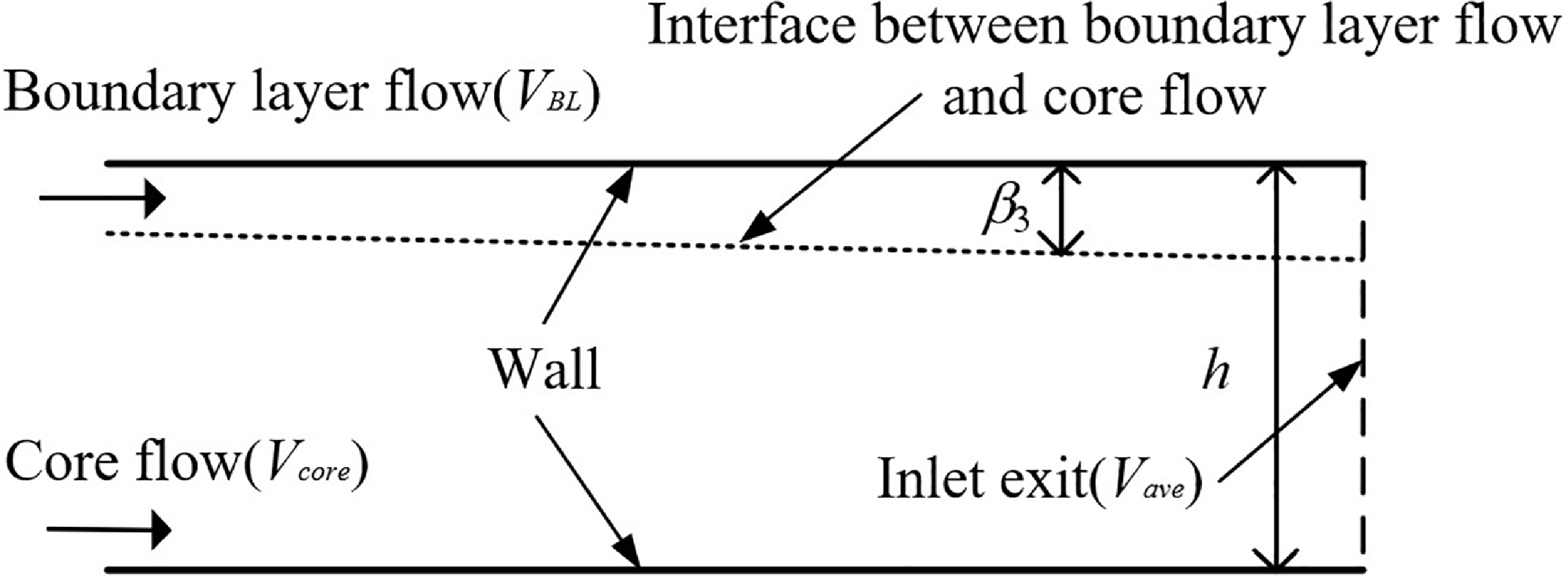
After considering the boundary layer, the fluid at the exit of the inlet is composed of two parts: a low-energy fluid within the boundary layer and a high-energy fluid within the core flow. If we only consider the core flow, it is obviously not in line with the actual situation. In order to consider the influence of the boundary layer, this paper proposes a uniformisation model for the fluid parameters at the exit of the inlet, which averages the fluid within the boundary layer and the core flow based on their respective area ratio of the inlet exit. A schematic diagram is shown in Fig. 7. The computational approach for the uniformisation model is as follows: the velocity within the boundary layer near the wall is zero, and it gradually transitions to the core flow velocity based on some function relationship. This paper adopts an empirical power-law distribution pattern [Reference Najafi, Saidi, Sadeghipour and Souhar25], which is expressed as follows.
 \begin{align} {V}_{BL}(y)={V}_{core}^{*}{(y/{\beta }_{3})}^{\frac{1}{7}}\text{}(0\le y\le {\beta }_{3})\end{align}
Here, the subscript BL represents the boundary layer, and the subscript core represents the core flow.
 $\beta$
3
represents the height of the boundary layer, and y represents the distance of a certain point from the wall. After obtaining the thickness of the boundary layer, the average velocity of the fluid within the boundary layer can be expressed as follows.
 \begin{align} {V}_{BL}={\displaystyle {\int _{0}}^{{\beta }_{3}}{V}_{BL}}(y)dy/{\beta }_{3}\end{align}
Once the average velocity of the fluid within the boundary layer is obtained, the core flow velocity and the boundary layer velocity are averaged based on the area ratio, as shown in Equation (30).
 \begin{align} {V}_{ave}=({V}_{BL}\cdot {\beta }_{3}+{V}_{core}\cdot (h-{\beta }_{3}))/h\end{align}
In the equation, h represents the height of the exit of the inlet. As the core flow parameters are already known and the total temperature of the boundary layer and the total temperature of the core flow are equal, the mixed temperature T save can be determined based on the energy conservation Equation (31).
 \begin{align} {H}^{*}({T}_{t}{}_{ave})=H({T}_{save})+0.5{V}_{ave}^{2}\end{align}
Based on the relationship between static temperature and Mach number, the mixed Mach number Ma ave can be determined.
 \begin{align} {T}_{t}{}_{ave}={T}_{s}{}_{ave}\cdot \big(1+(\gamma -1)/2\cdot {M}_{ave}^{2}\big)\end{align}
In the equation,
 $ \gamma$
is the specific heat ratio. Based on the flow mass conservation, the total mixed pressure P
tave
can be obtained.
 \begin{align} m=\sqrt{\frac{\gamma }{R}{\bigg(\frac{2}{\gamma -1} \bigg)}^{\frac{\gamma +1}{\gamma -1}}}\cdot Pt{}_{ave}/\sqrt{T{t}_{ave}}\cdot q(M{a}_{ave})\cdot A\end{align}
In the equation, R is the gas constant. Then, calculate the mixed static pressure P save based on the relationship between total pressure and static pressure.
 \begin{align} {P}_{t}{}_{ave}={P}_{s}{}_{ave}\cdot {\big(1+(\gamma -1)/2\cdot M{a}_{ave}^{2}\big)}^{\frac{\gamma }{\gamma \text{-1}}}\end{align}
2.4 Definition of inlet performance parameters
To meet the needs of research and analysis, relevant performance parameters should be defined. The flow coefficient
 $ \varphi$
is used to evaluate the amount of freestream entering the inlet [Reference Van Wie, Curran and Murthy24]. It is defined as
 \begin{align} \varphi =\frac{m}{{m}_{0}}\end{align}
where m is the actual mass flow rate into the inlet, m 0 is the mass flow rate through the capture area in the freestream state.
The total pressure recovery coefficient
 $ \sigma$
is used to evaluate the loss of total pressure due to shock waves and viscosity [Reference Van Wie, Curran and Murthy24]. It is defined as
 \begin{align} \sigma \text{=}\frac{{P}_{t}}{{P}_{t}{}_{0}}\end{align}
where P t is the mean total pressure at the inlet exit, and P t0 is the freestream total pressure. The definition of the drag coefficient is shown as follows [Reference Van Wie, Curran and Murthy24].
 \begin{align} {C}_{x}=\frac{F}{\dfrac{1}{2}{\rho }_{\text{0}}{V}_{\text{0}}^{2}{A}_{\text{0}}}\end{align}
where F is the drag,
 $ \rho$
0 is the density of freestream, V0
is the velocity of freestream, A
0
is the capture area of the freestream. The definition of compression efficiency is given in Equation (38) [Reference Van Wie, Curran and Murthy24].
 \begin{align} {\eta }_{c}=\frac{{h}_{e}-{h}_{0}}{{h}_{3}-{h}_{0}}\end{align}
where h e represents the static enthalpy of the inflow at the inlet exit when isentropically expanded to the ambient pressure, h 0 denotes the total enthalpy of inflow, and h 3 represents the actual total enthalpy of the inlet exit.
3.0 CFD method and validation
3.1 CFD method
To verify the accuracy of the modeling approach, the CFD simulation will be utilised in this study first. The CFD calculations have reliable accuracy and can provide a large amount of data and all kinds of contours, which can be used to compare the model analysis from multiple perspectives, including both individual model comparisons and overall model comparisons.
The numerical simulation is performed based on the steady Reynolds-averaged Navier-Stokes (RANS) equations with the finite volume method and the shear stress transport (SST) k-
 $ \omega$
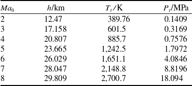
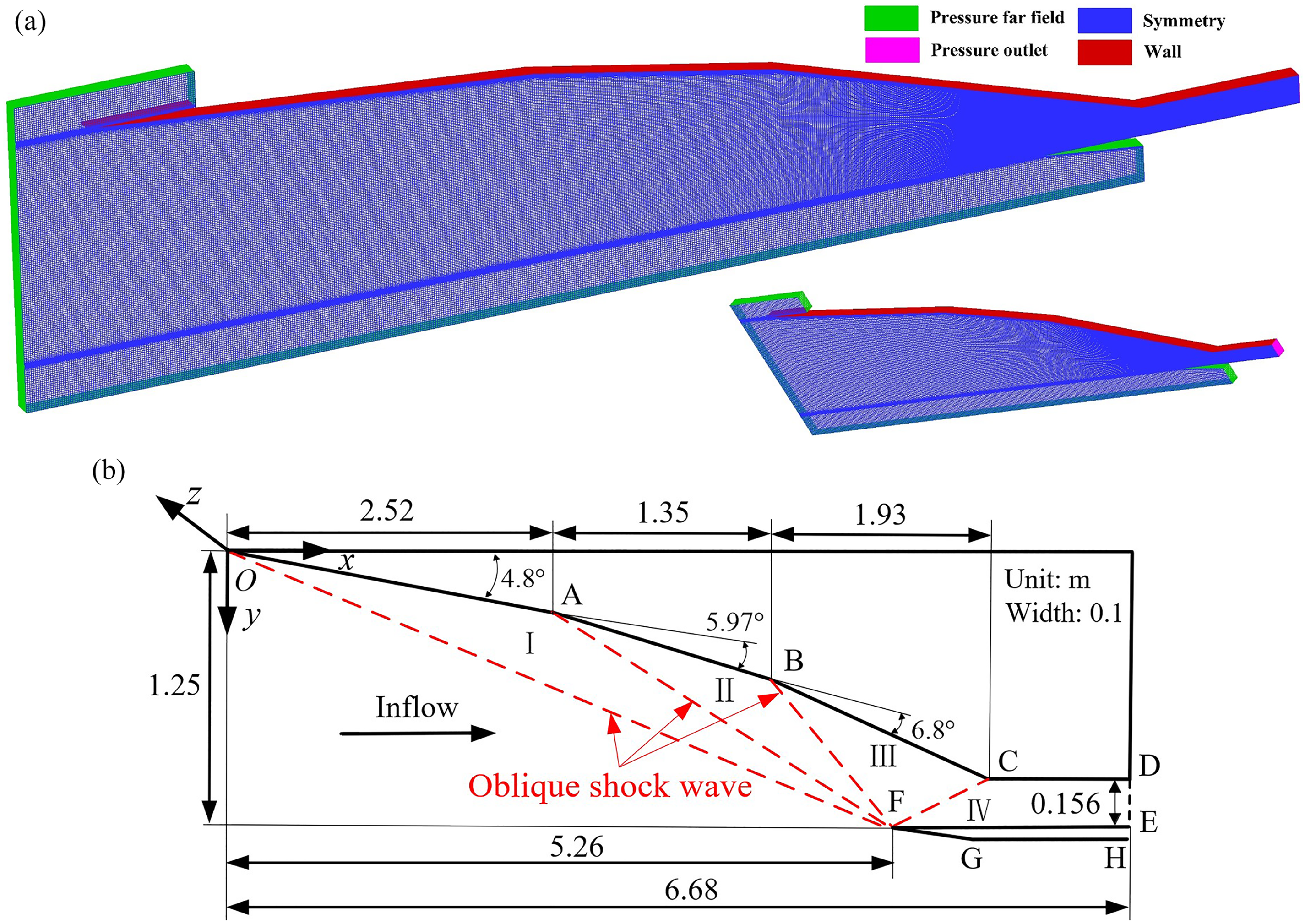
turbulence model. Its accuracy has been validated in many refs [Reference Li, Chang, Tang, Yu, Bao and Song26, Reference Shi, Chang, Zhang, Wang, Hou and Bao27]. To provide exact resolution of shock discontinuities, the advection upstream splitting method (AUSM) from the density-based solver is employed for the approximation of the convective flux splitting and the governing equations were discretised by the second-order upwind method. The density-based solver with second-order spatial accuracy is used for the implicit time-marching solution. The fluid is considered to be a single-species, calorically perfect air with the viscosity solved by Sutherland’s law. In the calculations, if the residuals of the equations drop to less than 10−4, the results are considered to be converged. The commercial software ICEM is used to discretise the computation domain with a structured grid. Among them, the inlet grid and size are shown in Fig. 8. The grid quality is 0.92, and the y
+ value is below 1.0. The average distance of the first cell centroid from the walls is 1 × 10⁻⁵ m. The stretching factor of the grid spacing is 1.1, which is beneficial to accurately capture the structures of the boundary layer. Moreover, the grid refinement processing has been done at the leading edge. In addition, the inflow conditions are provided in Table 3. Among them, Ma
0 is the inflow Mach number, h represents the flight altitude, Tt
denotes the total temperature and P
t
represents the total pressure.
Boundary conditions of inflow

Table 3. Long description
A table titled Boundary conditions of inflow with four columns and eight rows. The columns are labeled Ma0, h/km, Tt/K, and Pt/MPa. The rows present the following data: Row 1: Ma0, 2; h/km, 12.47; Tt/K, 389.76; Pt/MPa, 0.1409. Row 2: Ma0, 3; h/km, 17.158; Tt/K, 601.5; Pt/MPa, 0.3169. Row 3: Ma0, 4; h/km, 20.807; Tt/K, 885.7; Pt/MPa, 0.7576. Row 4: Ma0, 5; h/km, 23.665; Tt/K, 1,242.5; Pt/MPa, 1.7972. Row 5: Ma0, 6; h/km, 26.029; Tt/K, 1,651.1; Pt/MPa, 4.0846. Row 6: Ma0, 7; h/km, 28.047; Tt/K, 2,148.8; Pt/MPa, 8.8196. Row 7: Ma0, 8; h/km, 29.809; Tt/K, 2,700.7; Pt/MPa, 18.094. The table provides specific values for inflow Mach number, flight altitude, total temperature, and total pressure used in the numerical simulation based on the steady Reynolds-averaged Navier-Stokes equations.
Inlet mesh and size at design point: (a) inlet grid at design point (b) inlet size at design point.

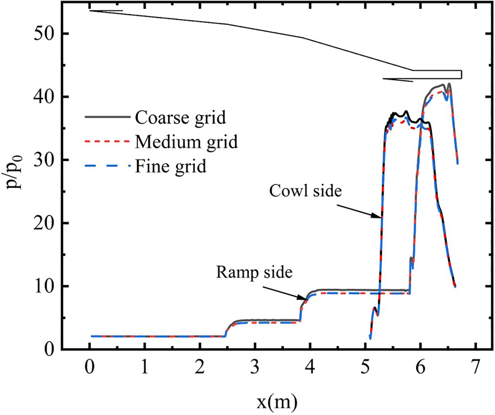
Meanwhile, in order to verify grid independence, a simulation of the above inlet with a coarse grid (3.3 m), fine grid (5.3 m) and dense grid (7.3 m) was done under the inflow condition of Mach 6. Figure 9 displays the comparison of static wall pressure (p is the static pressure and subscript ‘0’ denotes the freestream parameter) under different grid scales. It can be seen from the figure that the fine and dense grids show the same trend, and the coarse grid has a slight deviation. Therefore, the fine and dense grid represents more adequately the flow behaviour. Taking into account the calculation cost and simulation accuracy requirements, the fine grid with 5.3 m cells is finally chosen for subsequent simulations.
Comparison of static wall pressures under different grids.

3.2 CFD validation
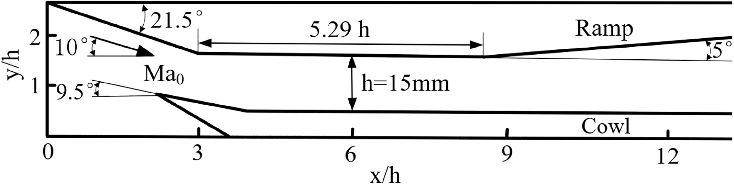
The CFD method is used to validate analysis models. However, its own accuracy should first be verified. To accomplish this, the inlet simulation in this study will be compared with Reinartz’s experimental results [Reference Herrmann and Koschel28, Reference Reinartz, Herrmann and Ballmann29]. These researchers conducted extensive experimental research on a two-dimensional mixed-compression inlet and obtained clear color schlieren photographs and wall pressure distribution. Figure 10 shows the inlet configuration without the first compression ramp. The second compression angle of the ramp of the inlet is
 $ \delta$
2
= 21.5°. The first compression angle is processed with the attack angle
 $ \alpha$
= −10°. The angle of the cowl is 9.5°, while the divergence angle behind the isolator is 5°. The isolator has a height h of 15 mm and a length of 5.29h (79.3 mm). Specific other structural dimensions can be found in Ref. [Reference Herrmann and Koschel28]. The inlet flow conditions are Mach number Ma
0
= 2.5, static pressure P
0
= 32896.52 Pa and static temperature T
0
= 131.47 K.
Simplified geometry configuration of the inlet.

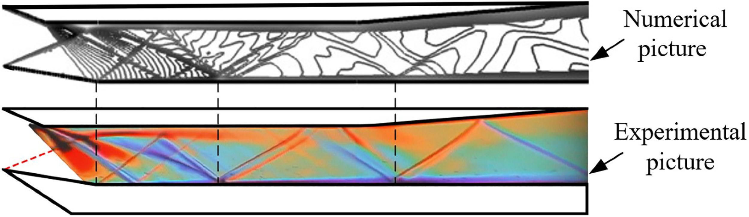
Figure 11 compares the density gradient picture from the numerical simulation of the inlet flow field with experimental schlieren results [Reference Dalle, Fotia and Driscoll15]. A fan-shaped expansion wave is generated when the airflow passes through the shoulder of the inlet, and the shock wave caused by the cowl corner impinges on the ramp across the separation shock and the reattachment shock. Compared with the schlieren image of the experimental testing, the numerical simulation captures the complex shock wave structures and separation regions within the inlet, and the flow structures are in good agreement.
Comparison between numerical and experimental schlieren pictures [Reference Dalle, Fotia and Driscoll15].

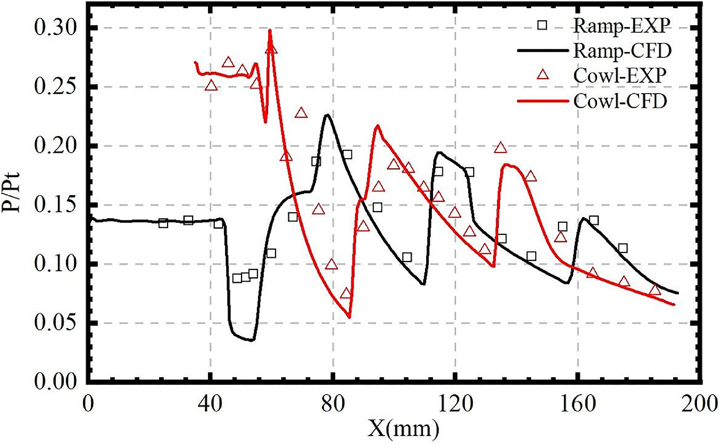
As illustrated in Fig. 12, the non-dimensional pressure distribution results from numerical simulations are compared with experimental data [Reference Dalle, Fotia and Driscoll15]. It can be observed that the non-dimensional pressure distributions of the two exhibit a similar variation trend, with a slight discrepancy. The discrepancy may be attributed to differences in the experimental and numerical computational conditions, such as the uniformity of the inflow conditions or errors in the eddy viscosity assumption. Overall, the numerical density gradient and wall pressure results match the experimental results well, indicating the correctness of the simulation method.
Comparison of simulation and experimental results on wall pressure distribution [Reference Dalle, Fotia and Driscoll15].

4.0 Results and discussion
4.1 Initial geometric design and analysis
The external compression system of the inlet designed in this study consists of three compression ramps, which are determined by a comprehensive consideration of the
 $ \sigma$
and structural dimensions. The more compression ramps, the closer the compression process approaches isentropic conditions, thereby enhancing the
 $ \sigma$
. However, this also leads to an increased inlet length. Empirical evidence suggests that, beyond four compression ramps, the increase of
 $ \sigma$
is relatively small. In addition, considering the complexity of the geometric structure, it is finally determined that the inlet design contains three external compression ramps. The sum of the three external compression angles is the
 $ \delta$
, which affects the compression efficiency of the inlet and is a design parameter that needs to be focused on. Another important design parameter is the CR, which directly affects the inlet starting ability. To comprehensively analyse the impact of both the
 $ \delta$
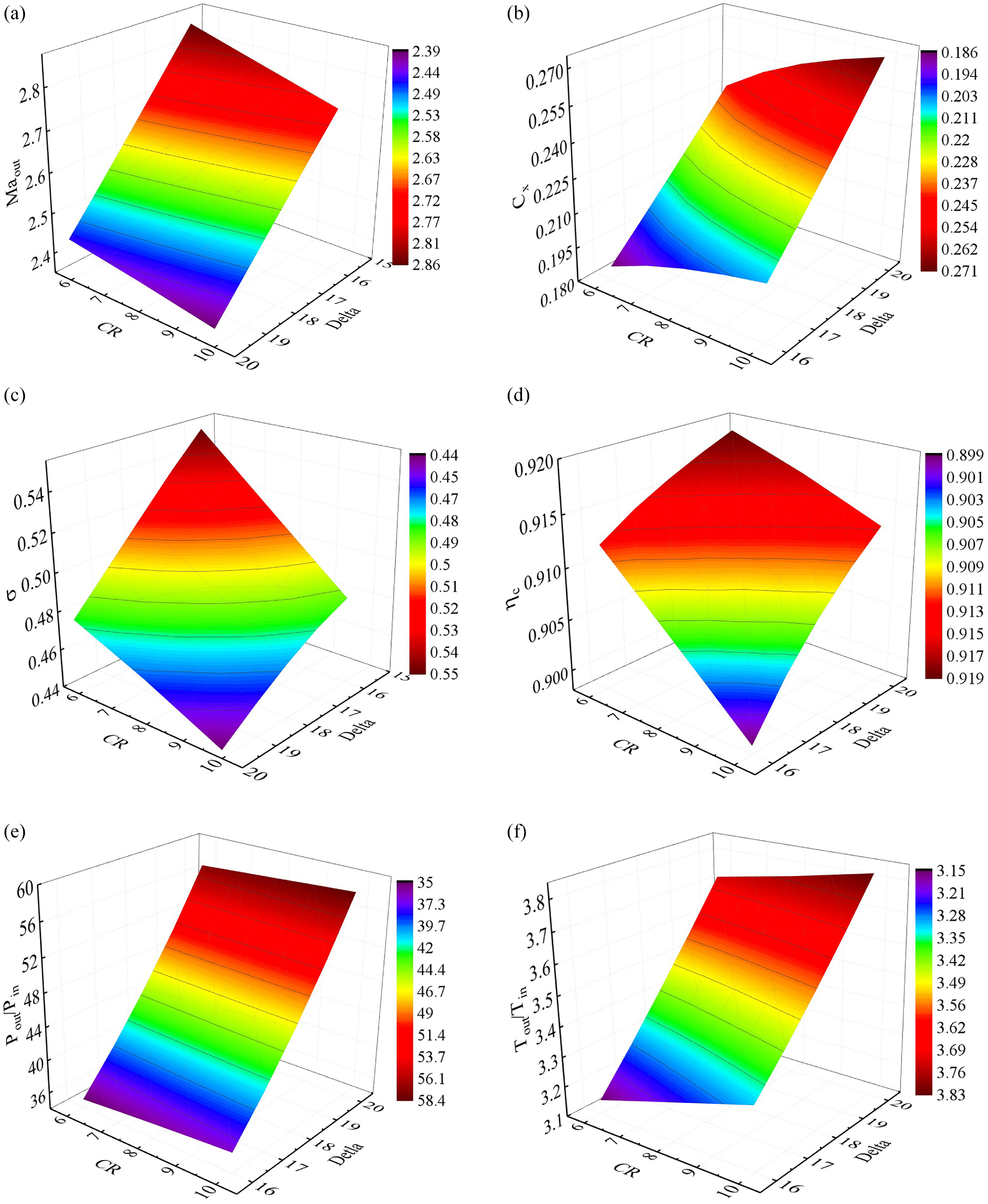
and CR on the inlet performance characteristics, Fig. 13 illustrates the variation of inlet performance parameters corresponding to two design parameters at the design-point Mach number of 6.
The inlet performance parameters with the total deflection angle and CR: (a) Mach number distribution (b) drag coefficient distribution (c) distribution of total pressure recovery coefficient (d) compression efficiency distribution (e) distribution of pressure rise ratio (f) distribution of temperature rise ratio.

Figure 13. Long description
Six 3D surface plots illustrate the distribution of various inlet performance parameters with total deflection angle and compression ratio. Panel A: A 3D surface plot shows the Mach number distribution. The x-axis represents the compression ratio (C R), the y-axis represents the total deflection angle (Delta), and the z-axis represents the Mach number. The color gradient ranges from purple to red, indicating varying Mach number values. Panel B: A 3D surface plot displays the drag coefficient distribution. The x-axis represents the compression ratio (C R), the y-axis represents the total deflection angle (Delta), and the z-axis represents the drag coefficient. The color gradient ranges from purple to red, indicating varying drag coefficient values. Panel C: A 3D surface plot illustrates the distribution of the total pressure recovery coefficient. The x-axis represents the compression ratio (C R), the y-axis represents the total deflection angle (Delta), and the z-axis represents the total pressure recovery coefficient. The color gradient ranges from purple to red, indicating varying total pressure recovery coefficient values. Panel D: A 3D surface plot shows the compression efficiency distribution. The x-axis represents the compression ratio (C R), the y-axis represents the total deflection angle (Delta), and the z-axis represents the compression efficiency. The color gradient ranges from purple to red, indicating varying compression efficiency values. Panel E: A 3D surface plot depicts the distribution of the pressure rise ratio. The x-axis represents the compression ratio (C R), the y-axis represents the total deflection angle (Delta), and the z-axis represents the pressure rise ratio. The color gradient ranges from purple to red, indicating varying pressure rise ratio values. Panel F: A 3D surface plot illustrates the distribution of the temperature rise ratio. The x-axis represents the compression ratio (C R), the y-axis represents the total deflection angle (Delta), and the z-axis represents the temperature rise ratio. The color gradient ranges from purple to red, indicating varying temperature rise ratio values.
It can be observed that increasing the CR of the inlet gradually enhances the degree of compression of the inflow, resulting in a decrease in the throat Mach number and
 $ \sigma$
, thereby increasing the pressure rise ratio and temperature rise ratio to some extent. However, the increase in the CR also leads to an increase in the inlet drag coefficient. This is because the compression of the freestream at the inlet gradually increases, and the pressure distribution on the inlet wall also gradually increases. At the same time, the projected area of the inlet along the drag direction also increases. As a result of the combined effect of these two factors, the inlet drag coefficient demonstrates a clear monotonic increasing trend. With the increase of the
 $ \delta$
, the external compression wave gradually strengthens, which directly leads to an increase in total pressure loss. Meanwhile, the pressure rise ratio and temperature rise ratio also gradually increase. As revealed by the above analysis, the CR and
 $ \delta$
show similar impact on inlet performance in a certain range.
When it comes to aerodynamic design, the
 $ \sigma$
is consistently prioritised as the core performance indicator. A higher
 $ \sigma$
signifies better performance, but the pursuit of excessively high values can result in a reduction in the pressure rise ratio and temperature rise ratio, leading to reduced combustion efficiency in the combustion chamber. Thus, a comprehensive weighing and selection of appropriate CR and
 $ \delta$
are necessary during the inlet design. Based on research and design objectives, the CR for this design is 8, with the
 $ \delta$
of 18°. All subsequent analyses are performed based on two design parameters.
4.2 Boundary layer modification design and analysis
Under supersonic inflow conditions, the influence of the boundary layer on the performance of the inlet cannot be ignored. Table 4 shows the impact of the boundary layer on the inlet performance at the design point conditions. It is observed that the inlet flow coefficient decreases when considering the boundary layer, indicating that the presence of the boundary layer leads to an increase in the external compression shock angle and the total pressure loss also increases accordingly. In addition, there is also a small increase in the pressure rise ratio and temperature rise ratio.
Comparison of inlet performance parameters with and without boundary layer

Table 4. Long description
A table comparing inlet performance parameters with and without boundary layer under supersonic inflow conditions. The table has two rows and six columns. The columns are labeled as Pout/Pin, Tout/Tin, Cx, φ, σ, and Maout. The row labels are No boundary layer and Boundary layer. Row 1: No boundary layer, Pout/Pin, 41.190; Tout/Tin, 3.264; Cx, 0.155; φ, 1; σ, 0.582; Maout, 2.751. Row 2: Boundary layer, Pout/Pin, 42.348; Tout/Tin, 3.290; Cx, 0.163; φ, 0.949; σ, 0.574; Maout, 2.726.
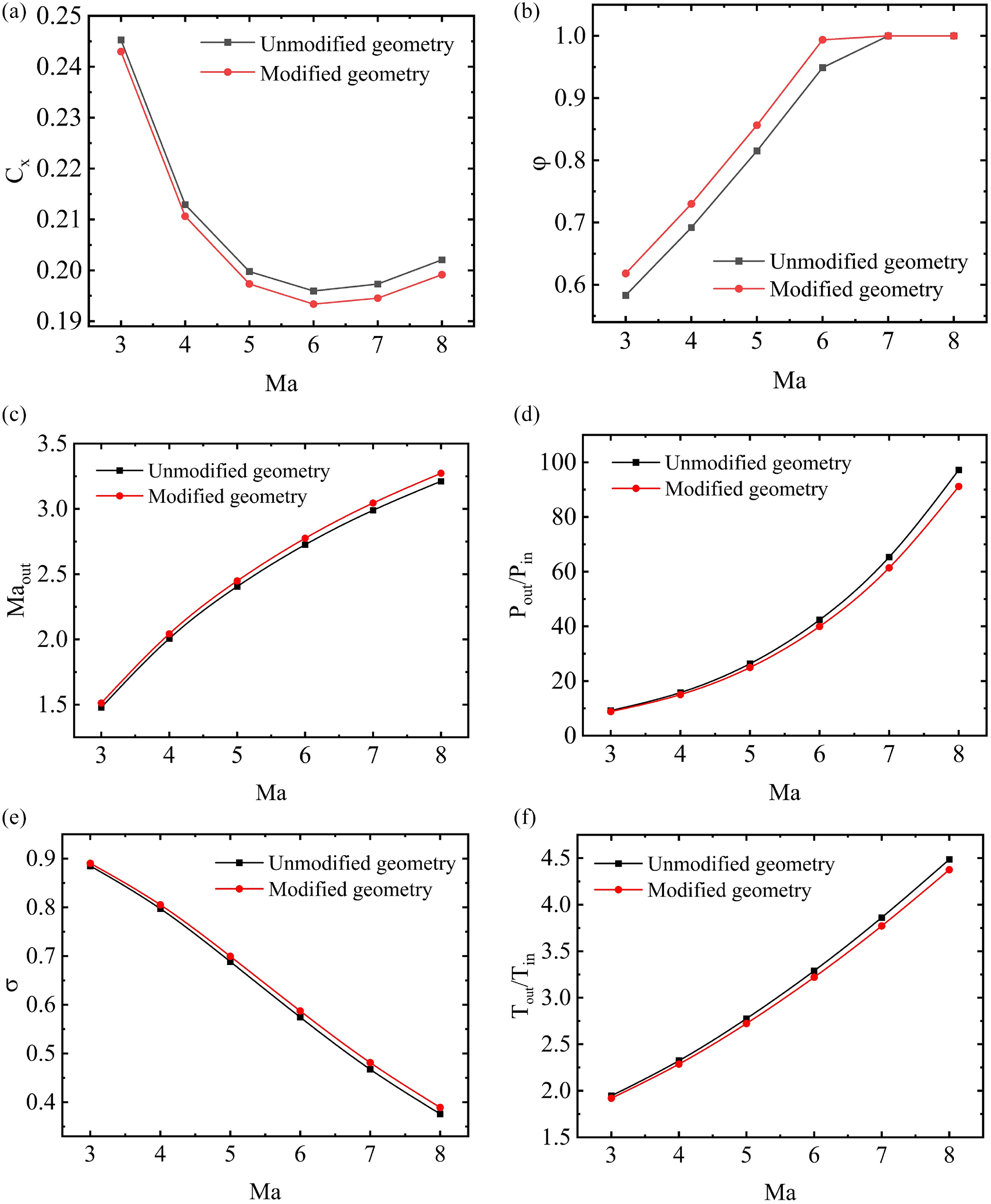
Performance parameter comparisons without and with boundary layer modification: (a) drag coefficient (b) flow coefficient (c) Mach number of inlet exit (d) pressure rise ratio (e) total pressure recovery coefficient (f) temperature rise ratio.

During the design stage of the inlet, neglecting the boundary layer may cause a deviation of the design point performance parameters from the actual values. The conventional approach is to design under inviscid conditions and then consider the effect of the boundary layer. Although this design method takes the boundary layer into account, the
 $ \varphi$
is still less than 1, which is not the design state we expected. The ideal design state should be such that the
 $ \varphi$
at the design point is equal to 1, and the compression oblique shock wave intersects at the lip of the cowl. In order to achieve the aforementioned design state, this study adopts the boundary layer modification method to modify the geometric ramps at the design point. The modified design is compared with the unmodified design in terms of performance parameters, as shown in Fig. 14. The modification results show a larger
 $ \sigma$
and a smaller drag coefficient, which are highly beneficial for the inlet performance. At the same time, it may be accompanied by a reduction in compression angle and an increase in exit Mach number. However, from the perspective of the importance of inlet performance parameters, the
 $ \varphi$
has a larger impact on inlet performance and should be prioritised. Clearly, the inlet modified with boundary layer modification exhibits better performance.
After considering the boundary layer, the fluid in the inlet will be divided into the low-speed fluid in the boundary layer and the high-speed fluid in the core flow. The current simplified approach is to ignore the low-speed fluid and only treat the core flow as the final fluid at the inlet exit, which inevitably introduces a certain error. In order to reduce this error, this study proposes a uniformisation model that takes into account the influence of the boundary layer.
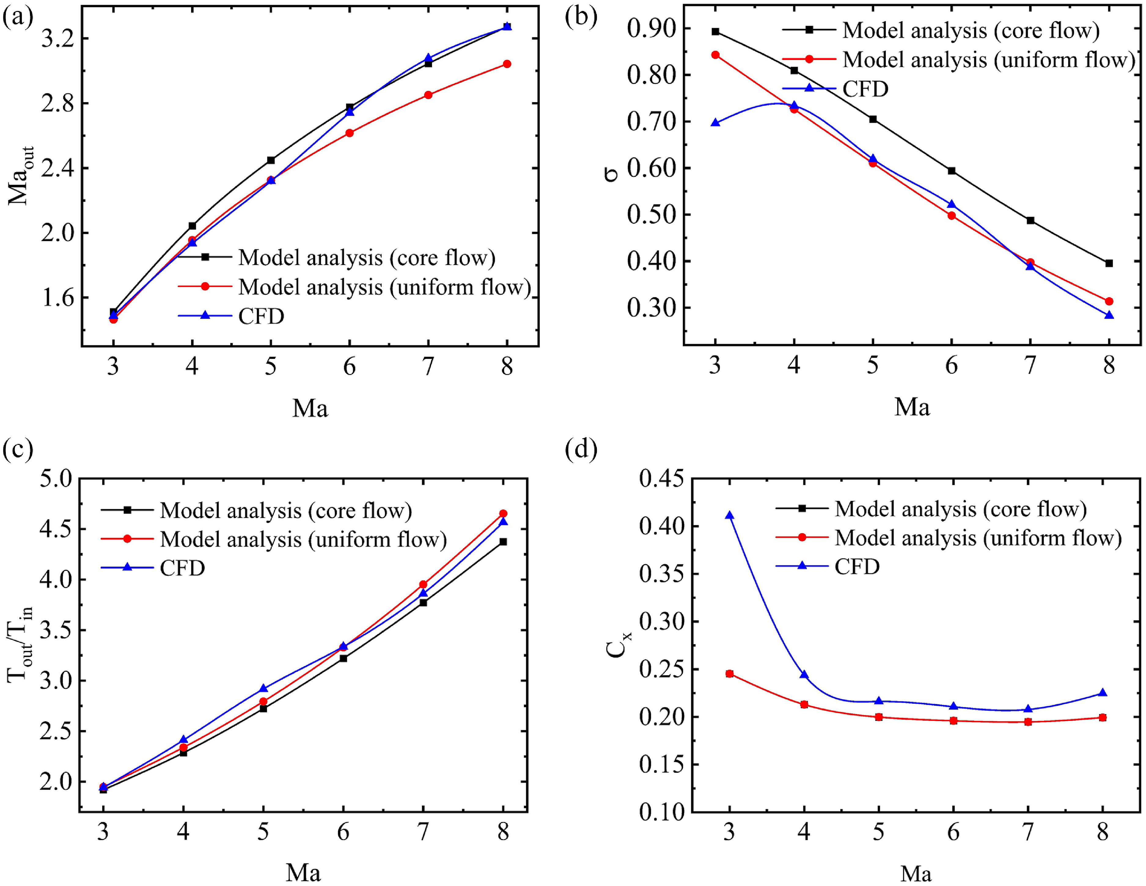
Figure 15 shows a comparison of the fluid parameters at the exit between the uniformisation model, the core flow simplification model and the CFD simulation results. The temperature rise ratio Tout
/Tin
and
 $ \sigma$
obtained using the uniformisation model are closer to the CFD results, while the Mach number obtained using the core flow model is more similar to the CFD results because the model analysis does not consider the effect of flow separation. During CFD simulation, flow separation occurs, and a decrease in flow area will lead to an increase in velocity, corresponding to a decrease in static pressure. In terms of the drag coefficient, the variation trend of model analysis and CFD simulation is generally consistent under different inflow conditions. However, there is a significant difference at low Mach numbers, which is due to the neglect of reflected shock waves and flow separation in the model analysis. Comparing the uniformisation model and the core flow model, it is found that the exit parameters obtained using the uniformisation model are closer to the CFD results. Moreover, it should be noted that the deviation between the model analysis and the CFD simulation increases as the Mach number increases, which may be due to the occurrence of an over-rated state under high Mach number inflow conditions. The model analysis cannot describe the coupling between shock waves and the boundary layer, nor can it consider the multiple reflections of shock waves inside the inlet. Thus, the discrepancy between the model analysis and CFD results increases as the Mach number increases.
Comparisons between the model analysis and CFD simulation: (a) Mach number of inlet exit (b) total pressure recovery coefficient (c) temperature rise ratio (d) drag coefficient.

4.3 Variable geometry design and analysis
The present study selects Mach 6 as the design point, which may encounter difficulties in self-starting under the low Mach number conditions. In consideration of variable geometry adjustment’s capability to directly alter the CR and improve its self-starting performance, the designed inlet will use variable geometry adjustment. Specifically, the angle of the third ramp will be adjusted to rotate upward in response to the decreasing Mach number of the inflow. Meanwhile, to maintain the original external compression system and ensure that the
 $ \varphi$
is not affected by the rotation of the final ramp, the rotation point H is not at the starting point of the final compression ramp. However, as the inflow Mach number decreases, the shock wave angle increases, and the
 $ \varphi$
still exhibits a rapid decrease. In order to obtain a relatively large flow coefficient under different inflow conditions, it is a reasonable choice to horizontally move the cowl. In the following analysis, the inlet performance is compared between the different variable geometry schemes, using the non-variable geometry performance as the benchmark.
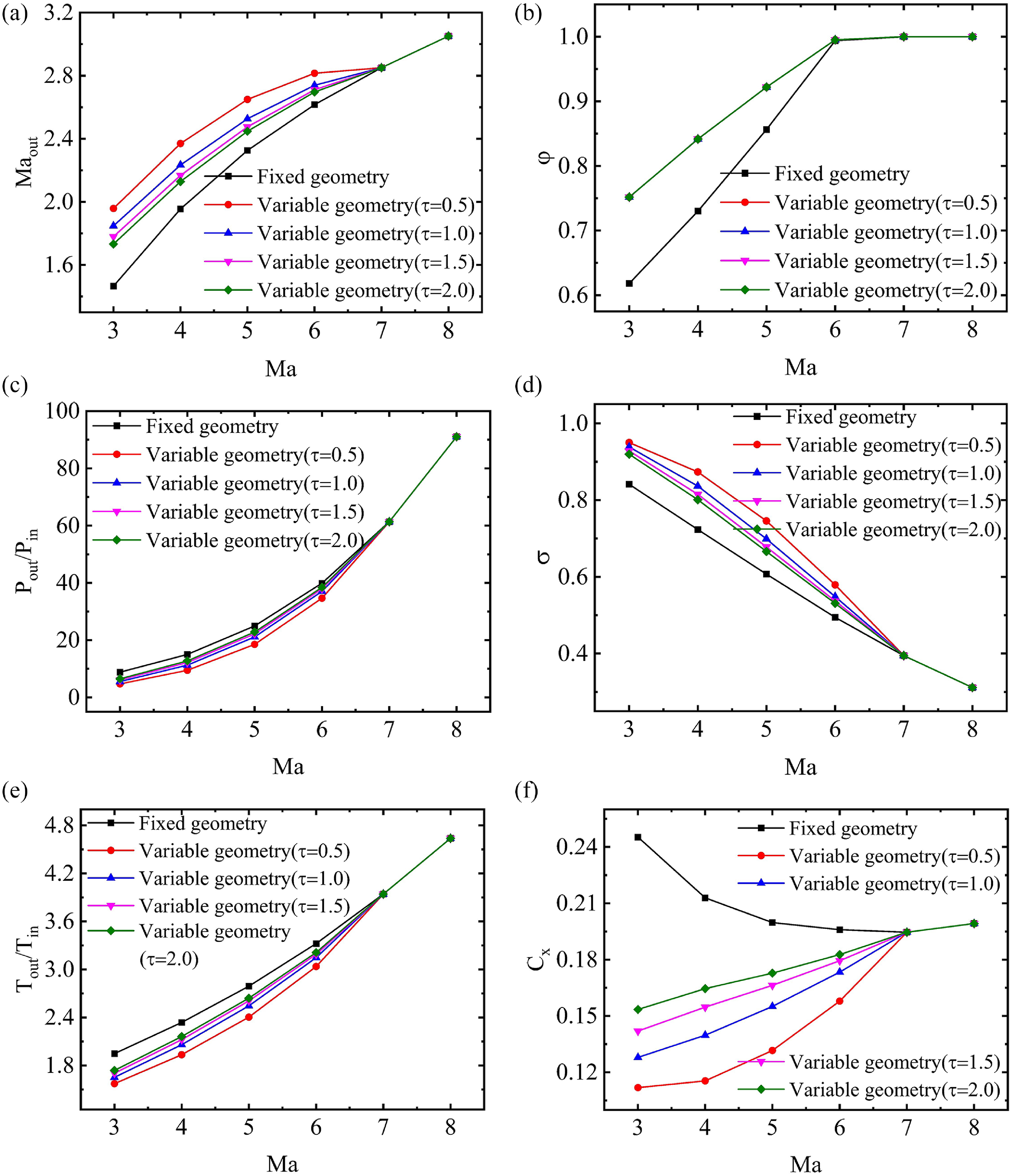
Performance parameter comparisons between the variable and fixed geometry inlet: (a) Mach number of inlet exit (b) flow coefficient (c) pressure rise ratio (d) total pressure recovery coefficient (e) temperature rise ratio (f) drag coefficient.

Figure 16. Long description
The image contains six line graphs comparing performance parameters between variable and fixed geometry inlets. Each graph represents different performance metrics plotted against the Mach number (Ma). Panel A: The graph shows the Mach number of the inlet exit (Ma_out) on the vertical axis and the Mach number (Ma) on the horizontal axis. The lines represent different geometries, including fixed geometry and variable geometries with different tau values (0.5, 1.0, 1.5, 2.0). Panel B: The graph shows the flow coefficient (phi) on the vertical axis and the Mach number (Ma) on the horizontal axis. The lines represent different geometries, similar to Panel A. Panel C: The graph shows the pressure rise ratio (P_out/P_in) on the vertical axis and the Mach number (Ma) on the horizontal axis. The lines represent different geometries, similar to Panel A. Panel D: The graph shows the total pressure recovery coefficient (sigma) on the vertical axis and the Mach number (Ma) on the horizontal axis. The lines represent different geometries, similar to Panel A. Panel E: The graph shows the temperature rise ratio (T_out/T_in) on the vertical axis and the Mach number (Ma) on the horizontal axis. The lines represent different geometries, similar to Panel A. Panel F: The graph shows the drag coefficient (C_d) on the vertical axis and the Mach number (Ma) on the horizontal axis. The lines represent different geometries, similar to Panel A. Each graph indicates that variable geometry inlets generally perform better across the entire operating range compared to fixed geometry inlets.
As depicted in Fig. 16, adjusting the rotation of the final ramp according to the
 $ \tau$
function leads to a decrease in the compression of the inflow compared to non-variable geometry. Consequently, variable geometry can enhance the
 $ \sigma$
and Mach number at the throat, while reducing the pressure rise ratio and temperature rise ratio. In particular, the drag coefficient is reduced, which is very beneficial to the engine. Moreover, the smaller the
 $ \tau$
value, the smaller the drag coefficient. However, the
 $ \varphi$
is independent of the value of
 $ \tau$
. This is because the external compression shock waves remain unchanged under different variable geometry schemes. As the inflow Mach number increases, the
 $ \varphi$
increases, which is determined by the position of the cowl lip. In general, performance parameters of variable geometry with the larger
 $ \tau$
value are closer to the fixed geometry inlet. Thus, it is recommended not to set
 $ \tau$
to a value that is too high, to avoid the inlet unstart under the low-speed inflow conditions.
Comparison of performance parameters between model analysis and CFD simulation

Table 5. Long description
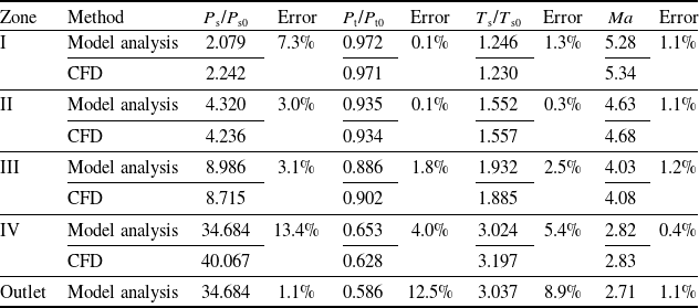
A table comparing performance parameters between model analysis and CFD simulation across different zones. The table has 6 rows and 7 columns. The columns are labeled as Zone, Method, Ps/Ps0, Error, Pt/Pt0, Error, Ts/Ts0, Error, Ma, and Error. The rows are labeled with zones I, II, III, IV, and Outlet, and methods Model analysis and CFD. Row 1: Zone I, Model analysis, Ps/Ps0 2.079, Error 7.3 percent, Pt/Pt0 0.972, Error 0.1 percent, Ts/Ts0 1.246, Error 1.3 percent, Ma 5.28, Error 1.1 percent. Row 2: Zone I, CFD, Ps/Ps0 2.242, Pt/Pt0 0.971, Ts/Ts0 1.230, Ma 5.34. Row 3: Zone II, Model analysis, Ps/Ps0 4.320, Error 3.0 percent, Pt/Pt0 0.935, Error 0.1 percent, Ts/Ts0 1.552, Error 0.3 percent, Ma 4.63, Error 1.1 percent. Row 4: Zone II, CFD, Ps/Ps0 4.236, Pt/Pt0 0.934, Ts/Ts0 1.557, Ma 4.68. Row 5: Zone III, Model analysis, Ps/Ps0 8.986, Error 3.1 percent, Pt/Pt0 0.886, Error 1.8 percent, Ts/Ts0 1.932, Error 2.5 percent, Ma 4.03, Error 1.2 percent. Row 6: Zone III, CFD, Ps/Ps0 8.715, Pt/Pt0 0.902, Ts/Ts0 1.885, Ma 4.08. Row 7: Zone IV, Model analysis, Ps/Ps0 34.684, Error 13.4 percent, Pt/Pt0 0.653, Error 4.0 percent, Ts/Ts0 3.024, Error 5.4 percent, Ma 2.82, Error 0.4 percent. Row 8: Zone IV, CFD, Ps/Ps0 40.067, Pt/Pt0 0.628, Ts/Ts0 3.197, Ma 2.83. Row 9: Outlet, Model analysis, Ps/Ps0 34.684, Error 1.1 percent, Pt/Pt0 0.586, Error 12.5 percent, Ts/Ts0 3.037, Error 8.9 percent, Ma 2.71, Error 1.1 percent.
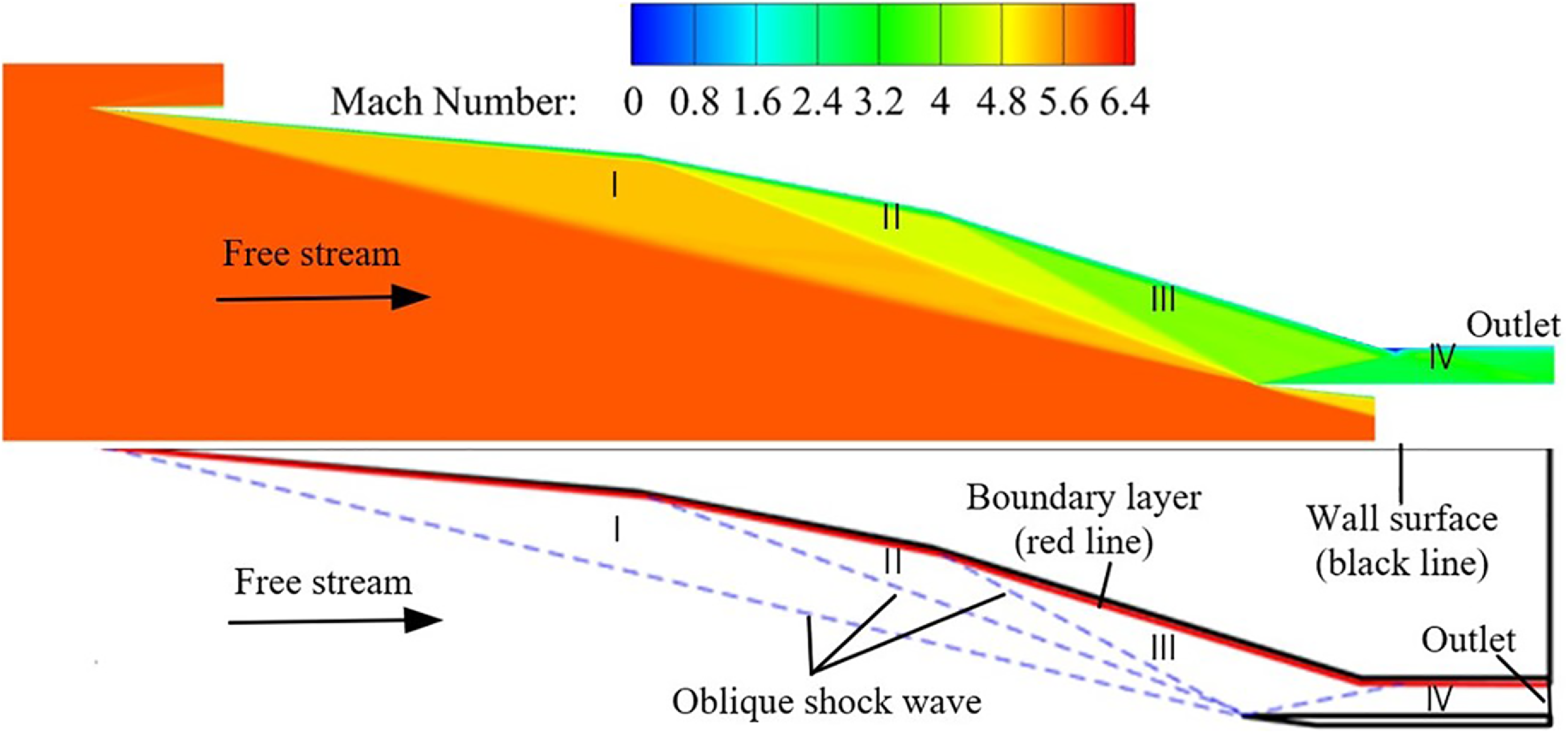
Shock wave comparison between model analysis and CFD simulation.

4.4 Verification of the variable geometry design
4.4.1 Model verification
When a supersonic fluid encounters the compression ramp of the inlet, a shock wave will be generated, and after the shock wave, the fluid parameters will change. According to the position of the shock wave, the fluid parameters in the inlet can be divided into different regions. In this study, the external compression section of the inlet contains three ramps that generate three oblique shock waves, and a fourth shock wave is generated at the lip of the cowl. Figure 17 shows a comparison between the results of the model analysis and CFD simulation at the design point. Comparing the shock wave of the model analysis at the design point condition with the CFD simulation, it is found that external compression shock waves intersect at the cowl lip. Furthermore, a comparison result of the downstream flow parameters after the shock wave reveals a maximum deviation of approximately 14% (as shown in Table 5), which floats within an acceptable range.
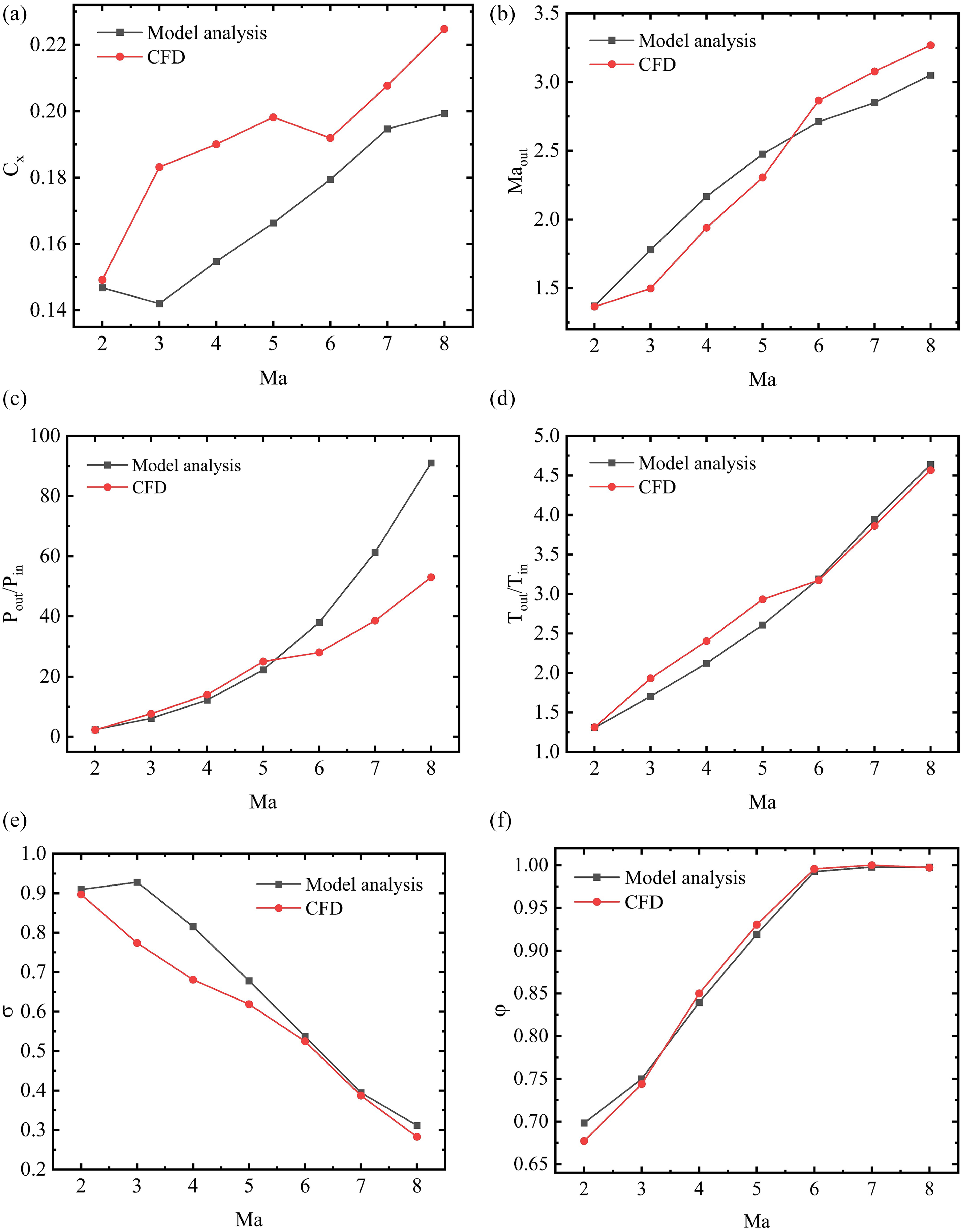
Performance parameter comparisons between the model analysis and CFD simulation: (a) drag coefficient (b) Mach number of inlet exit (c) pressure rise ratio (d) temperature rise ratio (e) total pressure recovery coefficient (f) flow coefficient.

Figure 18. Long description
The image contains six line graphs comparing performance parameters between model analysis and CFD simulation. Each graph plots data against the Mach number (Ma) on the horizontal axis. Panel A: The first graph shows the drag coefficient (Cf) on the vertical axis. The drag coefficient increases with the Mach number for both model analysis and CFD simulation, with CFD values generally higher. Panel B: The second graph depicts the Mach number of the inlet exit (Ma_out) on the vertical axis. Both model analysis and CFD simulation show an increasing trend with the Mach number, with CFD values slightly higher. Panel C: The third graph illustrates the pressure rise ratio (P_out/P_in) on the vertical axis. Both datasets show an increasing trend with the Mach number, with model analysis values higher than CFD values. Panel D: The fourth graph presents the temperature rise ratio (T_out/T_in) on the vertical axis. Both datasets show an increasing trend with the Mach number, with CFD values slightly higher. Panel E: The fifth graph shows the total pressure recovery coefficient (σ) on the vertical axis. Both datasets show a decreasing trend with the Mach number, with model analysis values higher than CFD values. Panel F: The sixth graph depicts the flow coefficient (φ) on the vertical axis. Both datasets show an increasing trend with the Mach number, with CFD values slightly higher.
4.4.2 Verification of variable geometry results
To verify the reliability of variable geometry inlet performance established with the analysis model, a comparison is conducted between the analysis model and CFD simulations under the condition of the variable geometry adjustment law of
 $ \tau$
= 1.5. The comparative findings are illustrated in Fig. 18. The variation trend of parameter
 $ \varphi$
from the analytical model exhibits substantial consistency with that obtained via CFD simulations, further validating the rationality of the boundary layer modification design. However, noticeable discrepancies are observed in the remaining performance parameters. Notably, the C
x
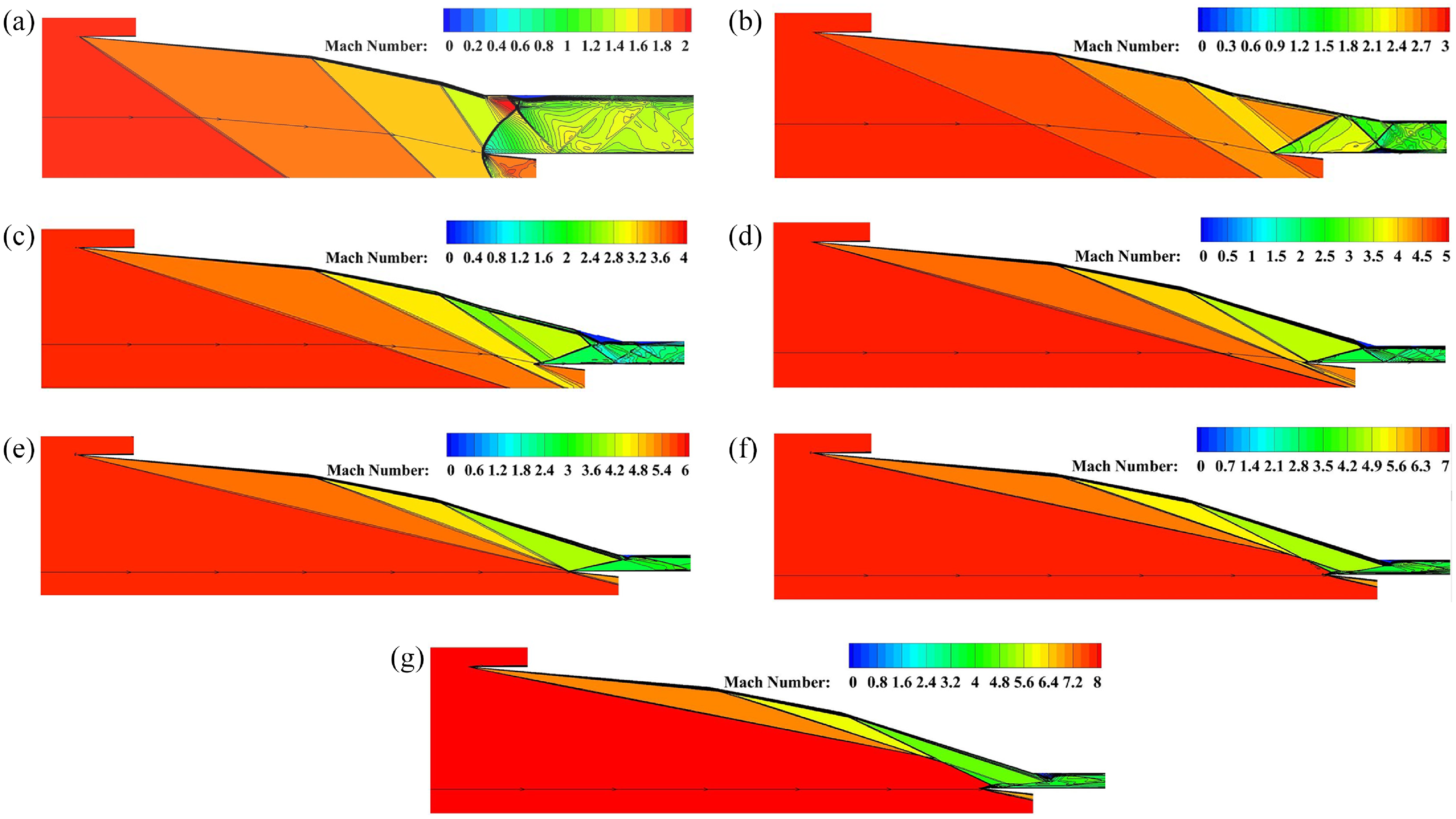
obtained from the two calculations under the inflow Mach 3 ∼ 6 exhibits significant discrepancy. This discrepancy can primarily be attributed to the formation of a reflected shock wave on the variable ramp shown in Fig. 19, leading to an increase in wall pressure. However, the analysis model cannot take into account the effects of this reflected shock wave. In terms of the pressure rise ratio at the exit of the inlet, the deviation is seen when the inflow Mach number ranges from 5 to 8. As shown in Fig. 19, complex flow separation occurs at the throat of the inlet, accompanied by the interaction between shock waves and expansion waves. However, such flow separation and shock wave interaction were not taken into account in the analysis model, resulting in the above deviations. Upon further analysis, it can be observed that when the cowl-lip shock wave interacts with the boundary layer on the side of the compression ramp, flow separation will take place. Nevertheless, the degree of flow separation varies under different inflow conditions. In some cases, it is a significant flow separation, while in other cases, it is a relatively minor one. Figure 19(b) to (d) illustrates the occurrence of large flow separation, and this flow separation induces a new shock wave. The new shock wave, together with the cowl-lip shock wave, is reflected multiple times within the channel, resulting in a complex wave system structure, which leads to a substantial total pressure loss. Consequently, in this state, there is a certain error between the analysis model and CFD calculation, especially in terms of the total pressure recovery coefficient and the drag coefficient. However, Fig. 19(a) shows a smaller flow separation, and the intensity of the reflected shock wave is also weak. In this state, the performance parameters of the inlet obtained through model analysis and CFD calculation are in good agreement. Clearly, the coupling effect between the shock wave and the boundary layer is the crucial factor causing the error. Overall, the analysis model can generally reflect the performance of the variable geometry inlet at different inflow conditions. In the future, the error between model calculation and CFD calculation can be further reduced by establishing the coupling model of cowl-lip shock wave and boundary layer.
Mach number contours of wide-speed-range variable geometry inlet: (a) inflow condition of Mach 2 (b) inflow condition of Mach 3 (c) inflow condition of Mach 4 (d) inflow condition of Mach 5 (e) inflow condition of Mach 6 (f) inflow condition of Mach 7 (g) inflow condition of Mach 8.

5.0 Conclusions
This paper introduces a systematic design method for wide-speed-range inlets, developed based on a one-dimensional model, and validates its reliability through comprehensive numerical simulations. The core insights and conclusions resulting from this work are summarised as follows.
Regarding the boundary layer modification design, the results demonstrate that implementation of this innovative configuration yields a significantly higher total pressure recovery coefficient and a correspondingly lower drag coefficient – both of which represent substantial performance enhancements for the inlet system. Furthermore, a novel uniformisation model that explicitly accounts for boundary layer effects in the calculation of inlet exit parameters is proposed. Comparative analysis against high-fidelity numerical simulation results confirms that this proposed uniformisation model produces predictions that closely align with the calculation data, outperforming traditional approaches that neglect boundary layer influences.
From the validation perspective of the design point, comparative analysis of shock wave distributions between the one-dimensional model and numerical simulations reveals consistent intersection of the primary shock waves at the cowl lip. Quantitative assessment of post-shock downstream flow parameters further demonstrates a maximum deviation of approximately 14%, which floats within an acceptable range. This strong correlation between analytical predictions and computational results provides robust confirmation of the design method’s reliability and accuracy.
Off-design point validation of the design method is performed by comparing one-dimensional model results with numerical simulations under the
 $ \tau$
= 1.5 variable geometry adjustment condition. The analysis shows the model correctly predicts the general trend of inlet performance parameter changes, but quantitative differences exist in specific values. A comprehensive numerical investigation demonstrates that these discrepancies primarily arise from flow separation induced by the coupling between the cowl-lip shock wave and the boundary layer.
Competing interests
The authors declare that they have no known competing financial interests or personal relationships that could have appeared to influence the work reported in this paper.