1. Introduction
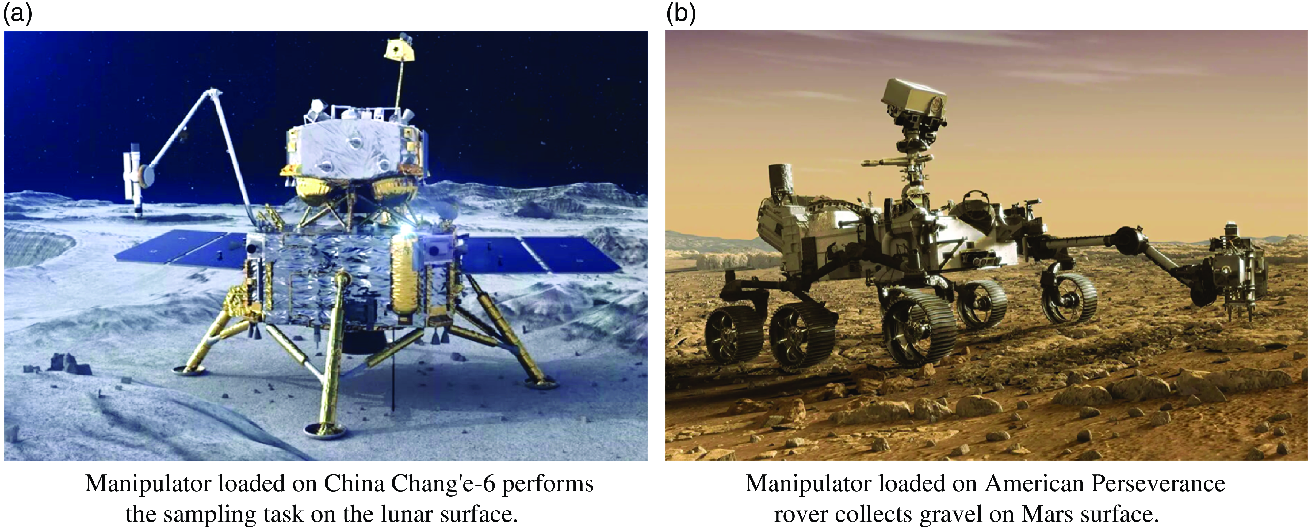
With the advancement of aerospace technology and the ongoing escalation of international competition in space, space activities of major space-faring nations are becoming increasingly frequent and are progressively shifting towards the planetary development [Reference Kuramoto, Kawakatsu, Fujimoto, Araya, Barucci, Genda, Hirata, Ikeda, Imamura, Helbert, Kameda, Kobayashi, Kusano, Lawrence, Matsumoto, Michel, Miyamoto, Morota, Nakagawa, Nakamura, Ogawa, Otake, Ozaki, Russell, Sasaki, Sawada, Senshu, Tachibana, Terada, Ulamec, Usui, Wada, Watanabe and Yokota1–Reference Li, Zhang, Yu, Zhang, Yu, Dong, Liu, Geng, Sun, Yan, Ren, Su, Zuo, Zhang, Cao, Fang, Yang, Shu, Lin, Zou, Liu, Liu, Kong, Zhu and Ouyang3]. As core equipment for planetary development tasks, planetary surface manipulators have played a critical role in a series of significant space missions, including lunar sample return and Mars surface sampling [Reference Verma, Hartman, Rankin, Del Sesto, Toupet, Graser, Myint, Davis, Klein, Koch, Brooks, Bailey, Justice, Dolci and Ono4–Reference Paz-Delgado, Sánchez-Ibáñez, Domínguez, Pérez-Del-Pulgar, Kirchner and García-Cerezo6], as shown in Figure 1. The objective of manipulator trajectory optimization is to generate smooth motion trajectories and iteratively optimizing trajectory parameters, thereby allowing the manipulator to transition smoothly and efficiently from the initial to the goal configuration by track the reference trajectory [Reference Ata7, Reference Gasparetto and Zanotto8]. For planetary surface manipulators, to execute more operational tasks within strictly limited time windows, the state trajectories should not only satisfy smoothness but also minimize the duration of the trajectory taken by the manipulator to move from the initial configuration to the goal configuration for each task, thereby improving operational efficiency [Reference Otsu, Agha-Mohammadi and Paton9, Reference Schmidt, Landis and Oleson10]. Additionally, considering the limited power supply available on planetary surfaces, the motion trajectory should maximize energy efficiency and minimize energy consumption [Reference Fallah, Yue, Vahid-Araghi and Khajepour11–Reference Schuster, Brunner, Bussmann, Büttner, Dömel, Hellerer, Lehner, Lehner, Porges, Reill, Riedel, Vayugundla, Vodermayer, Bodenmüller, Brand, Friedl, Grixa, Hirschmüller, Kaßecker, Márton, Nissler, Ruess, Suppaand and Wedler13]. However, minimizing trajectory duration and energy consumption are conflicting objectives; improving one often leads to the deterioration of the other. No solution that can simultaneously optimize both performance metrics, necessitating trade-off decisions between them to achieve a comprehensive optimization of trajectory duration and energy consumption. Therefore, it is essential to investigate multi-objective trajectory optimization under multiple constraints to enable planetary surface manipulators to perform tasks with high energy efficiency.
Planetary surface manipulators perform operation tasks.

Traditional trajectory optimization methods typically convert multi-objective problems into single-objective ones through non-negative weighted summation, necessitating the pre-establishment of relative importance weights for each performance metric [Reference Liu, Du, Wu, Liu and Li14, Reference Gregory, Olivares and Staffetti15]. However, accurately determining these weights in practical scenarios is challenging and often relies on empirical adjustments. Additionally, the differing dimensions and wide-ranging values among objectives require significant variation in weights, which can undermine the robustness of the optimal solution [Reference Zhang and Shi16]. Furthermore, single-objective optimization yields only one optimal solution, failing to reflect the interrelationships among multiple objectives, thereby diminishing the interpretability of the results.
In recent years, researchers have addressed the limitations of traditional trajectory optimization methods by proposing various bio-inspired multi-objective optimization algorithms, such as the multi-objective whale optimization algorithm [Reference Sanprasit and Artrit17–Reference Shanmugasundar, Fegade, Mahdal and Kalita19], multi-objective particle swarm optimization (MOPSO) [Reference Tripathi, Bandyopadhyay and Pal20–Reference Lan, Xie, Liu and Cao22], and multi-objective gray wolf optimization [Reference Liu, Yang and Li23–Reference Mirjalili, Saremi, Mirjalili and and Coelho25]. These algorithms simulate the collaborative foraging behaviors of natural swarms, such as fish, birds, and bees, to achieve complex intelligent search patterns. They provide non-dominated feasible solution sets and Pareto front through multi-objective cooperative optimization, enhancing the robustness and interpretability of results while facilitating the analysis of inter-objective relationships. Among these, the MOPSO employs a parallel exploration mechanism and information-sharing among particles to iterate towards better solutions, remaining unaffected by the shape of the objective space or characteristics of the cost function. It is widely applicable to multi-objective optimization problems in continuous spaces [Reference Hu, Zhang and Gong26–Reference Cheraghi and Jahangir28].
However, existing MOPSO algorithms typically necessitate that decision-makers predefine search ranges for the decision space based on experience. In addressing the specific issue of optimizing trajectory efficiency for manipulators, the appropriate setting of search ranges for each dimension of particles can significantly shorten convergence time in iterative optimization and mitigate the risk of falling into local optima. To avoid missing superior solutions, these ranges are often set excessively wide to comprehensively encompass all potential optimal solutions [Reference Tripathi, Bandyopadhyay and Pal20, Reference Chettibi29]. Yet, such expansive decision spaces significantly increase the number of ineffective explorations conducted by particle swarms, thereby diminishing the optimization efficiency of particle swarm algorithms. Hence, there is an urgent need to propose a strategy to adaptively adjust the boundaries of the multi-dimensional decision space, thereby improving the efficiency of particle swarm optimization.
Moreover, existing MOPSO algorithms typically maintain a single external archive. After each iteration, all feasible solutions that satisfy constraints are added to the external archive and undergo non-dominated sorting, while infeasible solutions are discarded directly [Reference Cao, Yan, Huang, Ai, Xu, Fu and Zou21, Reference Lan, Xie, Liu and Cao22]. However, infeasible solutions also contain valuable information, particularly those near constraint boundaries. Such solutions may even be closer to the true Pareto front than the feasible solutions in the archive. Discarding such “promising” infeasible solutions is regrettable. Thus, it is necessary to develop a strategy to accelerate convergence and improve solution accuracy by leveraging infeasible solutions, thereby enhancing the optimization capabilities of the algorithm, which has not yet been considered.
Besides, to achieve a Pareto front that is as evenly distributed and comprehensively covered as possible, existing optimization algorithms typically rank all non-dominated feasible solutions using crowding distance, guiding the particle swarm to prioritize regions where non-dominated feasible solutions are sparsely distributed by setting fixed multiples of nearest neighbor distances at both ends [Reference Cheraghi and Jahangir28, Reference Dao, Ngo, Pan and and Nguyen30]. However, these methods lack adaptability to the trends in the distribution of non-dominated feasible solutions. This study considers scenarios in which the slopes of lines fitted near multiple non-dominated feasible solutions at the endpoints approach zero, indicating that further exploration along the corresponding cost function directions has nearly reached its limit. At such points, it is unnecessary to redirect the particle swarm to focus on these areas. Therefore, developing a strategy to prevent ineffective iterations and reduce computational overhead is significant.
Motivated by the above considerations, we introduce an adaptive boundary adjustment strategy for adjusting the boundaries of the multi-dimensional decision space, which precisely regulates the time intervals between adjacent configuration nodes. Additionally, we construct two external archives – one for storing non-dominated feasible solutions and another for non-dominated infeasible solutions – to bridge the feasible and infeasible domains. This approach leverages information from infeasible solutions near the constraint boundaries to heuristically guide the particle swarm in efficiently exploring these regions, significantly improving the evolutionary optimization capability of the swarm and yielding a greater number of high-quality non-dominated solutions. Furthermore, we propose a swarm optimal position updating strategy based on sparsity sorting, which directs the swarm to explore areas where the distribution of non-dominated solutions along the Pareto front is sparse. This ensures the uniformity and completeness of the final Pareto front obtained through the algorithm. Finally, we integrate these improvements into a heuristic multi-objective particle swarm optimization (HMOPSO) algorithm and apply it alongside advanced algorithms such as NSGA-II, NSWOA, and MOGWO to the multi-objective trajectory optimization task for planetary surface manipulators. Comparative experiments validate the feasibility and superiority of the proposed HMOPSO algorithm. The contributions of this paper are as follows:
1) An adaptive boundary adjustment strategy is designed to achieve precise adaptation of the multi-dimensional decision space boundaries by specifically regulating the time intervals between adjacent configuration nodes.
2) A complementary dual-archive guided boundary exploration strategy is developed by constructing two complementary archives that connect the feasible and infeasible domains, thereby heuristically guiding the particle swarm to explore regions close to these boundaries. Consequently, the evolutionary optimization capability of the particle swarm is significantly enhanced.
3) A swarm optimal position updating strategy based on sparsity sorting is designed to guide the particle swarm toward areas on the Pareto front where non-dominated solutions are sparsely distributed, ensuring the uniformity and completeness of the final Pareto front.
4) An energy-efficient trajectory optimization algorithm HMOPSO is constructed based on the aforementioned strategies. Experimental results demonstrate that HMOPSO significantly outperform existing optimization algorithms in evolutionary optimization capabilities and convergence rates.
The remainder of this paper is organized as follows. Section 2 models the problem of energy-efficient trajectory optimization for manipulators. Section 3 presents the heuristic improvement strategies for the MOPSO algorithm. Section 4 describes the experiment setup and discusses the experimental results. Section 5 concludes this paper with some suggestions for further research.
2. Modeling the problem of energy-efficient trajectory optimization for manipulators
The core concept of trajectory optimization for manipulators involves adjusting the timing
 $T_{i}\,(i=1,2,\cdots, N)$
at which the manipulator passes through a specified series of configuration node
 $Q_{i}$
or modifying the time intervals between adjacent configuration nodes. A quintic B-spline curve is utilized for trajectory fitting, ensuring that the optimized trajectory maintains smoothness and adheres to specified kinematic and dynamic constraints. This optimization aims to minimize trajectory duration and energy consumption while achieving comprehensive performance objectives. The multi-objective trajectory optimization model for manipulators consists of design variables, decision vector, objective vector, and constraint conditions.
(1) design variables
The variable
 $h_{i}$
representing the time consumed for the
 $i$
-th segment of the trajectory denotes the motion time interval for the manipulator between the configuration nodes
 $Q_{i}$
and
 $Q_{i+1}$
.
 \begin{equation} h_{i}=T_{i+1}-T_{i}, i=1,2,\ldots, N_{h} \end{equation}
where
 $T_{i}$
denotes the time that manipulator passes through the configuration node
 $Q_{i}$
. The parameter
 $N_{h}$
represents the dimension of design variables,
 $N_{h}=N-1$
.
(2) decision vector
The decision vector
 $\boldsymbol{X}$
, composed of all
 $N_{h}$
variables
 $h_{i}(i=1,2,\ldots, N_{h})$
, has a dimension of
 $N_{h}$
. The
 $N_{h}$
-dimensional space formed by the decision vector
 $\boldsymbol{X}$
is referred to as the decision space.
 \begin{equation} \boldsymbol{X}=\left[\boldsymbol{h}_{\mathbf{1}},\boldsymbol{h}_{\mathbf{2}},\ldots, \boldsymbol{h}_{\boldsymbol{i}},\ldots, \boldsymbol{h}_{{\boldsymbol{N}_{\boldsymbol{h}}}}\right] \end{equation}
where the range of each variable
 $h_{i}$
is constrained by
 $h_{i\_ \min }\leq h_{i}\leq h_{i\_ \max }, i=1,2,\cdots, N_{h}$
.
(3) objective vector
The primary objective of energy-efficient trajectory optimization for manipulators is to minimize the time cost function and the energy cost function. To facilitate the unified representation of multiple cost functions, the objective vector
 $\boldsymbol{G}(\boldsymbol{X})$
is constructed as
 \begin{equation} \boldsymbol{G}\left(\boldsymbol{X}\right)=\left[\boldsymbol{g}_{\mathbf{1}}\left(\boldsymbol{X}\right),\boldsymbol{g}_{\mathbf{2}}\left(\boldsymbol{X}\right)\right] \end{equation}
 \begin{equation} \boldsymbol{g}_{\mathbf{1}}\left(\boldsymbol{X}\right)=\sum _{\boldsymbol{i}=\mathbf{1}}^{\boldsymbol{N}_{\boldsymbol{h}}}\boldsymbol{h}_{\boldsymbol{i}} \end{equation}
 \begin{equation} \boldsymbol{g}_{\mathbf{2}}\left(\boldsymbol{X}\right)=\int _{\mathbf{0}}^{\boldsymbol{T}}\left| \boldsymbol{\tau }^{\boldsymbol{T}}\dot{\boldsymbol{\Theta }}\right| \boldsymbol{dt} \end{equation}
where
 $\boldsymbol{G}(\boldsymbol{X})$
represents the objective vector. The function
 $g_{1}(\boldsymbol{X})$
is the time cost function, which indicates the total duration for the manipulator to move from the initial pose to the goal pose, serving as an efficiency performance metric. During operations, the manipulator should complete tasks in the shortest time possible to enhance operational efficiency. The function
 $g_{2}(\boldsymbol{X})$
denotes the energy cost function, representing the total energy consumption during the manipulator’s motion and measuring energy efficiency. Unlike existing trajectory optimization algorithms that commonly utilize simplified surrogate models to calculate the energy cost function, this paper employs the dynamic model to accurately compute the joint torques
 $\boldsymbol{\tau }$
and the energy cost function
 $g_{2}(\boldsymbol{X})$
. This approach ensures the reliability of the trajectory optimization results, and the computed joint torques can be directly used to verify whether the trajectory adheres to joint torque constraints.
(4) constraint conditions
The motion states of each joint of the manipulator must always adhere to specified constraints, including joint angular displacement, joint angular velocity, joint angular acceleration, joint angular jerk, and joint torque, throughout the entire motion process. The constraints can be expressed as
Joint angular displacement constraints:
 $| \mathbf{\Theta }(i)| \leq \mathbf{\Theta }_{\max }(i), i=1,2,\ldots, n$
Joint angular velocity constraints:
 $| \dot{\mathbf{\Theta }}(i)| \leq \dot{\mathbf{\Theta }}_{\max }(i), i=1,2,\ldots, n$
Joint angular acceleration constraints:
 $| \ddot{\mathbf{\Theta }}(i)| \leq \ddot{\mathbf{\Theta }}_{\max }(i), i=1,2,\ldots, n$
Joint angular jerk constraints:
 $| \dddot {\mathbf{\Theta }}(i)| \leq \dddot {\mathbf{\Theta }}_{\max }(i), i=1,2,\ldots, n$
Joint torque constraints:
 $| \boldsymbol{\tau }(i)| \leq \boldsymbol{\tau }_{\max }(i), i=1,2,\ldots, n$
To facilitate the unified computation and assessment of all constraints, the constraint violation function
 $\boldsymbol{F}(\boldsymbol{X})$
is designed as
 \begin{equation} \boldsymbol{F}\left(\boldsymbol{X}\right)=\boldsymbol{f}_{\boldsymbol{p}}\left(\boldsymbol{X}\right)+\boldsymbol{f}_{\boldsymbol{v}}\left(\boldsymbol{X}\right)+\boldsymbol{f}_{\boldsymbol{a}}\left(\boldsymbol{X}\right)+\boldsymbol{f}_{\boldsymbol{j}}\left(\boldsymbol{X}\right)+\boldsymbol{f}_{\boldsymbol{\tau }}\left(\boldsymbol{X}\right) \end{equation}
where the expression for each constraint penalty function is given by
 \begin{equation} \boldsymbol{f}_{\boldsymbol{p}}\left(\boldsymbol{X}\right)=\sum _{\boldsymbol{i}=\mathbf{1}}^{\boldsymbol{n}}\boldsymbol{Relu}\left(\frac{\boldsymbol{\max } \left(\left| \boldsymbol{S}_{\boldsymbol{\Theta }}\left(\boldsymbol{i},\boldsymbol{t}\right)\right| \right)-\boldsymbol{\Theta }_{\boldsymbol{\max }}\left(\boldsymbol{i}\right)}{\boldsymbol{\Theta }_{\boldsymbol{\max }}\left(\boldsymbol{i}\right)}\right) \end{equation}
 \begin{equation} \boldsymbol{f}_{\boldsymbol{v}}\left(\boldsymbol{X}\right)=\sum _{\boldsymbol{i}=\mathbf{1}}^{\boldsymbol{n}}\boldsymbol{Relu}\left(\frac{\boldsymbol{\max } \left(\left| \boldsymbol{S}_{\dot{\boldsymbol{\Theta }}}\left(\boldsymbol{i},\boldsymbol{t}\right)\right| \right)-\dot{\boldsymbol{\Theta }}_{\boldsymbol{\max }}\left(\boldsymbol{i}\right)}{\dot{\boldsymbol{\Theta }}_{\boldsymbol{\max }}\left(\boldsymbol{i}\right)}\right) \end{equation}
 \begin{equation} \boldsymbol{f}_{\boldsymbol{a}}\left(\boldsymbol{X}\right)=\sum _{\boldsymbol{i}=\mathbf{1}}^{\boldsymbol{n}}\boldsymbol{Relu}\left(\frac{\boldsymbol{\max } \left(\left| \boldsymbol{S}_{\ddot{\boldsymbol{\Theta }}}\left(\boldsymbol{i},\boldsymbol{t}\right)\right| \right)-\ddot{\boldsymbol{\Theta }}_{\boldsymbol{\max }}\left(\boldsymbol{i}\right)}{\ddot{\boldsymbol{\Theta }}_{\boldsymbol{\max }}\left(\boldsymbol{i}\right)}\right) \end{equation}
 \begin{equation} \boldsymbol{f}_{\boldsymbol{j}}\left(\boldsymbol{X}\right)=\sum _{\boldsymbol{i}=\mathbf{1}}^{\boldsymbol{n}}\boldsymbol{Relu}\left(\frac{\boldsymbol{\max } \left(\left| \boldsymbol{S}_{\dddot {\boldsymbol{\Theta }}}\left(\boldsymbol{i},\boldsymbol{t}\right)\right| \right)-\dddot {\boldsymbol{\Theta }}_{\boldsymbol{\max }}\left(\boldsymbol{i}\right)}{\dddot {\boldsymbol{\Theta }}_{\boldsymbol{\max }}\left(\boldsymbol{i}\right)}\right) \end{equation}
 \begin{equation} \boldsymbol{f}_{\boldsymbol{\tau }}\left(\boldsymbol{X}\right)=\sum _{\boldsymbol{i}=\mathbf{1}}^{\boldsymbol{n}}\boldsymbol{Relu}\left(\frac{\boldsymbol{\max } \left(\left| \boldsymbol{S}_{\boldsymbol{\tau }}\left(\boldsymbol{i},\boldsymbol{t}\right)\right| \right)-\boldsymbol{\tau }_{\boldsymbol{\max }}\left(\boldsymbol{i}\right)}{\boldsymbol{\tau }_{\boldsymbol{\max }}\left(\boldsymbol{i}\right)}\right) \end{equation}
where
 $\boldsymbol{S}_{\mathbf{\Theta }},\boldsymbol{S}_{\dot{\mathbf{\Theta }}},\boldsymbol{S}_{\ddot{\mathbf{\Theta }}},\boldsymbol{S}_{\dddot {\mathbf{\Theta }}},\boldsymbol{S}_{\boldsymbol{\tau }}$
represent the trajectory curves of joint angular displacement, joint angular velocity, joint angular acceleration, joint angular jerk, and joint torque of the manipulator. Here,
 $i$
denotes the joint index of the manipulator, and
 $t$
indicates the time at which the manipulator moves along the trajectory. The function
 $\mathbf{Relu}(x)$
outputs the input value when it is positive and outputs zero for any negative input, that is,
 $\mathbf{Relu}(x)=\begin{cases} 0, x\lt 0\\ x, x\geq 0 \end{cases}$
.
3. Heuristic improvement strategies for MOPSO algorithm
The fundamental principle of the MOPSO algorithm is to model optimization problems as the search for optimal positions within a decision space by a swarm of particles. Through a parallel exploration mechanism and a collaborative information-sharing technique, the particles iteratively and adaptively seek better solutions. The process begins with the initialization of a set of particles, where each particle’s position represents a potential solution to the optimization problem. Each particle searches for improved positions in the decision space and shares its current individual best position with others. All particles adjust their exploration velocities based on both the individual and global best positions, subsequently updating their positions iteratively. After numerous iterations, a set of non-dominated feasible solutions is obtained, representing a Pareto front in the objective space, with each non-dominated solution corresponding to a set of optimal trajectory parameters for planetary surface manipulators. The core of the MOPSO algorithm lies in the formulas for updating particle velocities and positions.
The velocity update formula for the
 $j$
-th particle in the (
 $k+1$
)-th iteration is defined as
 \begin{equation} \boldsymbol{V}_{\boldsymbol{j},\boldsymbol{k}+\mathbf{1}}=\boldsymbol{\omega }_{\boldsymbol{k}}\boldsymbol{V}_{\boldsymbol{j},\boldsymbol{k}}+\boldsymbol{r}_{\boldsymbol{p}}\boldsymbol{c}_{\boldsymbol{p},\boldsymbol{k}}\left(\boldsymbol{X}_{\boldsymbol{j},\boldsymbol{best}}-\boldsymbol{X}_{\boldsymbol{j},\boldsymbol{k}}\right)+\boldsymbol{r}_{\boldsymbol{q}}\boldsymbol{c}_{\boldsymbol{q},\boldsymbol{k}}\left(\boldsymbol{X}_{\boldsymbol{best}}-\boldsymbol{X}_{\boldsymbol{j},\boldsymbol{k}}\right) \end{equation}
To prevent excessive particle movement within a single iteration, it is necessary to constrain the maximum particle velocity using the following equation
 \begin{align} \boldsymbol{V}_{\boldsymbol{j},\boldsymbol{k}+\mathbf{1}}\left(\boldsymbol{i}\right)\Longleftarrow \begin{cases} \boldsymbol{V}_{\boldsymbol{j},\boldsymbol{k}+\mathbf{1}}\left(\boldsymbol{i}\right), \left| \boldsymbol{V}_{\boldsymbol{j},\boldsymbol{k}+\mathbf{1}}\left(\boldsymbol{i}\right)\right| \leq \boldsymbol{V}_{\boldsymbol{\max }}\\ \boldsymbol{V}_{\boldsymbol{\max }}\left(\boldsymbol{i}\right), \left| \boldsymbol{V}_{\boldsymbol{j},\boldsymbol{k}+\mathbf{1}}\left(\boldsymbol{i}\right)\right| \gt \boldsymbol{V}_{\boldsymbol{\max }} \end{cases}, \boldsymbol{i}=\mathbf{1,2},\ldots, \boldsymbol{N}_{\boldsymbol{h}} \end{align}
The formula for updating the position of the
 $j$
-th particle during the (
 $k+1$
)-th iteration is as
 \begin{equation} \boldsymbol{X}_{\boldsymbol{j},\boldsymbol{k}+\mathbf{1}}=\boldsymbol{X}_{\boldsymbol{j},\boldsymbol{k}}+\boldsymbol{V}_{\boldsymbol{j},\boldsymbol{k}+\mathbf{1}}, \boldsymbol{j}=\mathbf{1,2},\ldots, \boldsymbol{M}_{\boldsymbol{pop}} \end{equation}
To prevent particles from exceeding the boundaries of the decision space, it is necessary to constrain the particle positions using the following equation
 \begin{align} \boldsymbol{X}_{\boldsymbol{j},\boldsymbol{k}+\mathbf{1}}\left(\boldsymbol{i}\right)\Longleftarrow \begin{cases} \boldsymbol{X}_{\boldsymbol{\min }}\left(\boldsymbol{i}\right), \boldsymbol{X}_{\boldsymbol{j},\boldsymbol{k}+\mathbf{1}}\left(\boldsymbol{i}\right)\lt \boldsymbol{X}_{\boldsymbol{\min }}\left(\boldsymbol{i}\right)\\ \boldsymbol{X}_{\boldsymbol{j},\boldsymbol{k}+\mathbf{1}}\left(\boldsymbol{i}\right), \boldsymbol{X}_{\boldsymbol{\min }}\left(\boldsymbol{i}\right)\leq \boldsymbol{X}_{\boldsymbol{j},\boldsymbol{k}+\mathbf{1}}\left(\boldsymbol{i}\right)\leq \boldsymbol{X}_{\boldsymbol{\max }}\left(\boldsymbol{i}\right)\\ \boldsymbol{X}_{\boldsymbol{\max }}\left(\boldsymbol{i}\right), \boldsymbol{X}_{\boldsymbol{j},\boldsymbol{k}+\mathbf{1}}\left(\boldsymbol{i}\right)\gt \boldsymbol{X}_{\boldsymbol{\max }}\left(\boldsymbol{i}\right) \end{cases}, \boldsymbol{i}=\mathbf{1,2},\ldots, \boldsymbol{N}_{\boldsymbol{h}} \end{align}
where
 $M_{\mathrm{pop}}$
denotes the number of individual particles.
 $M_{k}$
represents the maximum number of iterations.
 $M_{g}$
represents the number of cost functions.
 $\omega _{k}$
represents the inertia weight, indicating the influence of the previous generation’s particle velocity on the current generation’s velocity.
 $c_{p,k}$
represents the cognitive learning factor, which reflects the particle’s reliance on its own historical best position.
 $c_{q,k}$
represents the social learning factor, reflecting a particle’s reliance on collective experience within the swarm. It adjusts the weight of a particle’s movement towards the swarm’s best position.
 $r_{p}$
and
 $r_{q}$
are random numbers within the interval
 $[0,1]$
, used to enhance the stochasticity and diversity in particle exploration processes.
 $\boldsymbol{V}_{j,k}$
denotes the velocity vector of particle
 $j$
during the
 $k$
-th iteration exploration.
 $\boldsymbol{X}_{j,k}$
represents the position vector of particle
 $j$
during the
 $k$
-th iteration exploration.
 $\boldsymbol{X}_{j,\text{best}}$
denotes the vector of the best historical position discovered by particle
 $j$
so far.
 $\boldsymbol{X}_{\text{best}}$
refers the best collective position discovered by the swarm up to the current iteration.
3.1 Adaptive boundary adjustment strategy of multi-dimensional decision space
In addressing the specific issue of optimizing trajectory efficiency for manipulators, the appropriate setting of search ranges for each dimension of particles can significantly shorten convergence time in iterative optimization and mitigate the risk of falling into local optima. However, traditional algorithms typically require decision-makers to predefine decision space search ranges based on experience. To avoid missing superior solutions, these ranges are often set excessively wide to encompass all potential optimal solutions comprehensively. Yet, such expansive decision spaces significantly increase the number of ineffective explorations by particle swarms, thereby diminishing the optimization efficiency of particle swarm algorithms. Consequently, this study proposes an adaptive strategy for adjusting boundaries of multi-dimensional decision spaces in multi-objective optimization. By incrementally adjusting time intervals between adjacent configuration nodes, the adaptive boundary adjustment strategy achieves adaptive adjustment of multi-dimensional decision space boundaries, thereby enhancing particle swarm optimization efficiency.
Firstly, for a given set of
 $N$
configuration nodes
 $Q_{i}(i=1,2,\ldots, N)$
, the minimum limit of the time interval between adjacent configuration nodes can be computed under the assumption that each joint of the manipulator operates at its maximum velocity throughout the trajectory.
 \begin{align} \boldsymbol{h}_{\boldsymbol{i},\mathbf{0}}= \mathop{\boldsymbol{\max}}\limits_{\boldsymbol{l}=\mathbf{1}\colon \boldsymbol{n}} \left\{\frac{\left| \boldsymbol{Q}_{\boldsymbol{i}+\mathbf{1}}\left(\boldsymbol{l}\right)-\boldsymbol{Q}_{\boldsymbol{i}}\left(\boldsymbol{l}\right)\right| }{\dot{\boldsymbol{\Theta }}_{\boldsymbol{\max }}\left(\boldsymbol{l}\right)}\right\}, \boldsymbol{i}=\mathbf{1,2},\ldots, \boldsymbol{N}_{\boldsymbol{h}} \end{align}
where
 $\dot{\mathbf{\Theta }}_{\max }(l)$
denotes the maximum allowable angular velocity of joint
 $l$
of the manipulator.
Then, non-uniform knots
 $\{u_{r}\}$
are constructed based on
 $N_{h}$
time intervals
 $h_{i,0}(i=1,2,\ldots, N_{h})$
.
 \begin{align} \boldsymbol{u}_{\boldsymbol{r}}=\begin{cases} & 0\,\,\,\,,\,\,\,\,\,\,\,\,\,\,\,\boldsymbol{r}=1,\ldots, \boldsymbol{q}+1\\ & \boldsymbol{u}_{\boldsymbol{r}-\mathbf{1}}+\frac{\boldsymbol{h}_{\boldsymbol{r}-\boldsymbol{q}-\mathbf{1,0}}}{\boldsymbol{T}_{\boldsymbol{h}}},\,\,\,\,\boldsymbol{r}=\boldsymbol{q}+2,\ldots, \boldsymbol{N}+\boldsymbol{q}-1\\ & 1\,\,\,\,\,,\,\,\,\,\,\,\,\,\,\,\boldsymbol{r}=\boldsymbol{N}+\boldsymbol{q},\ldots, \boldsymbol{N}+2\boldsymbol{q} \end{cases} \end{align}
where
 $T_{h}$
represents the total duration of the manipulator’s motion trajectory, that is,
 $T_{h}=\sum _{i=1}^{N_{h}}h_{i,0}$
.
Thus, the normalized non-uniform knot vector is obtained as
 \begin{equation} \mathrm{U}=\left\{\mathbf{u}_{\mathbf{r}}\right\}=\left\{\underset{\mathbf{q}+\mathbf{1}}{\underbrace{\mathbf{0,0},\ldots, \mathbf{0}}},\mathbf{u}_{\mathbf{q}+\mathbf{2}},\mathbf{u}_{\mathbf{q}+\mathbf{3}},\ldots, \mathbf{u}_{\mathbf{N}+\mathbf{q}-\mathbf{1}},\underset{\mathbf{q}+\mathbf{1}}{\underbrace{\mathbf{1,1},\ldots, \mathbf{1}}}\right\} \end{equation}
Subsequently, in conjunction with the
 $N$
configuration nodes
 $Q_{i}(i=1,2,\ldots, N)$
, the joint angular displacement, velocity, acceleration, and jerk trajectories of the manipulator are obtained using the quintic B-spline curve trajectory planning method. Afterwards, for each trajectory segment between adjacent nodes
 $Q_{i}$
and
 $Q_{i+1}(i=1,2,\ldots, N_{h})$
, the motion states of the manipulator’s joints are evaluated to determine if they consistently satisfy given constraints on joint angular displacement, velocity, acceleration, jerk, and torque. If any constraints are violated, the time interval between these two adjacent nodes
 $Q_{i}$
and
 $Q_{i+1}$
is adjusted accordingly.
 \begin{equation} \mathbf{h}_{\mathbf{i},\mathbf{0}}\leftarrow \mathbf{h}_{\mathbf{i},\mathbf{0}}+{\unicode[Arial]{x0394}} \mathbf{h}, \mathbf{if}\exists \mathbf{u}\in \left[\mathbf{u}_{\mathbf{i}+\mathbf{q}+\mathbf{1}},\mathbf{u}_{\mathbf{i}+\mathbf{q}+\mathbf{2}}\right], \mathbf{s}.\mathbf{t}. \mathbf{\beta }_{\boldsymbol{flag}}\left(\mathbf{u}\right)=\mathbf{1} \end{equation}
where
 $\beta _{\text{flag}}(u)$
denotes the constraint violation indicator, it takes the value 0 when the joint angular displacement
 , joint angular velocity
 $S\!\!\cdot\!\!{(u)}$
, joint angular acceleration
 , joint angular jerk
 , and joint torque
 all satisfy the specified constraints. Otherwise, if any of these conditions are not met,
 $\beta _{\text{flag}}(u)$
takes the value 1.
After each trajectory segment between adjacent configuration nodes on the entire path undergoes constraint verification and time interval updating, the normalized non-uniform knot vector
 $\boldsymbol{U}$
and the planned manipulator motion state trajectory curve are reconstructed based on the updated set of
 $N_{h}$
time intervals
 $h_{i,0}(i=1,2,\ldots, N_{h})$
. Subsequent constraint checks and interval updates are then performed again until the motion states at all points on the trajectory satisfy all constraints. Finally, the boundary expression of the multi-dimensional decision space obtained through adaptive adjustment is
 \begin{align} \begin{cases} \boldsymbol{h}_{\boldsymbol{i}\_ \boldsymbol{\min }}=\boldsymbol{\beta }_{\boldsymbol{\min }}\boldsymbol{h}_{\boldsymbol{i},\mathbf{0}}\\ \boldsymbol{h}_{\boldsymbol{i}\_ \boldsymbol{\max }}=\boldsymbol{\beta }_{\boldsymbol{\max }}\boldsymbol{h}_{\boldsymbol{i},\mathbf{0}} \end{cases}, \boldsymbol{i}=\mathbf{1,2},\ldots, \boldsymbol{N}_{\boldsymbol{h}} \end{align}
 \begin{equation} \boldsymbol{X}_{\boldsymbol{\min }}=\left[\boldsymbol{h}_{\mathbf{1}\_ \boldsymbol{\min }},\boldsymbol{h}_{\mathbf{2}\_ \boldsymbol{\min }},\ldots, \boldsymbol{h}_{\boldsymbol{i}\_ \boldsymbol{\min }},\ldots, \boldsymbol{h}_{{\boldsymbol{N}_{\boldsymbol{h}}}\_ \boldsymbol{\min }}\right] \end{equation}
 \begin{equation} \boldsymbol{X}_{\boldsymbol{\max }}=\left[\boldsymbol{h}_{\mathbf{1}\_ \boldsymbol{\max }},\boldsymbol{h}_{\mathbf{2}\_ \boldsymbol{\max }},\ldots, \boldsymbol{h}_{\boldsymbol{i}\_ \boldsymbol{\max }},\ldots, \boldsymbol{h}_{{\boldsymbol{N}_{\boldsymbol{h}}}\_ \boldsymbol{\max }}\right] \end{equation}
where the boundary scaling factors are set as
 $\beta _{\max }\gt 1$
,
 $0\lt \beta _{\min }\leq 1$
.
3.2 Complementary dual-archive guided boundary exploration strategy
Traditional multi-objective particle swarm optimization algorithms typically maintain a single external archive. After each iteration, all feasible solutions that satisfy constraints are added to the archive and undergo non-dominated sorting, while infeasible solutions are directly discarded. However, infeasible solutions also contain valuable information, especially those near constraint boundaries. These solutions may even be closer to the true Pareto front than the feasible solutions in the archive. Discarding such “promising” infeasible solutions is regrettable; leveraging them could significantly accelerate convergence and improve solution accuracy.
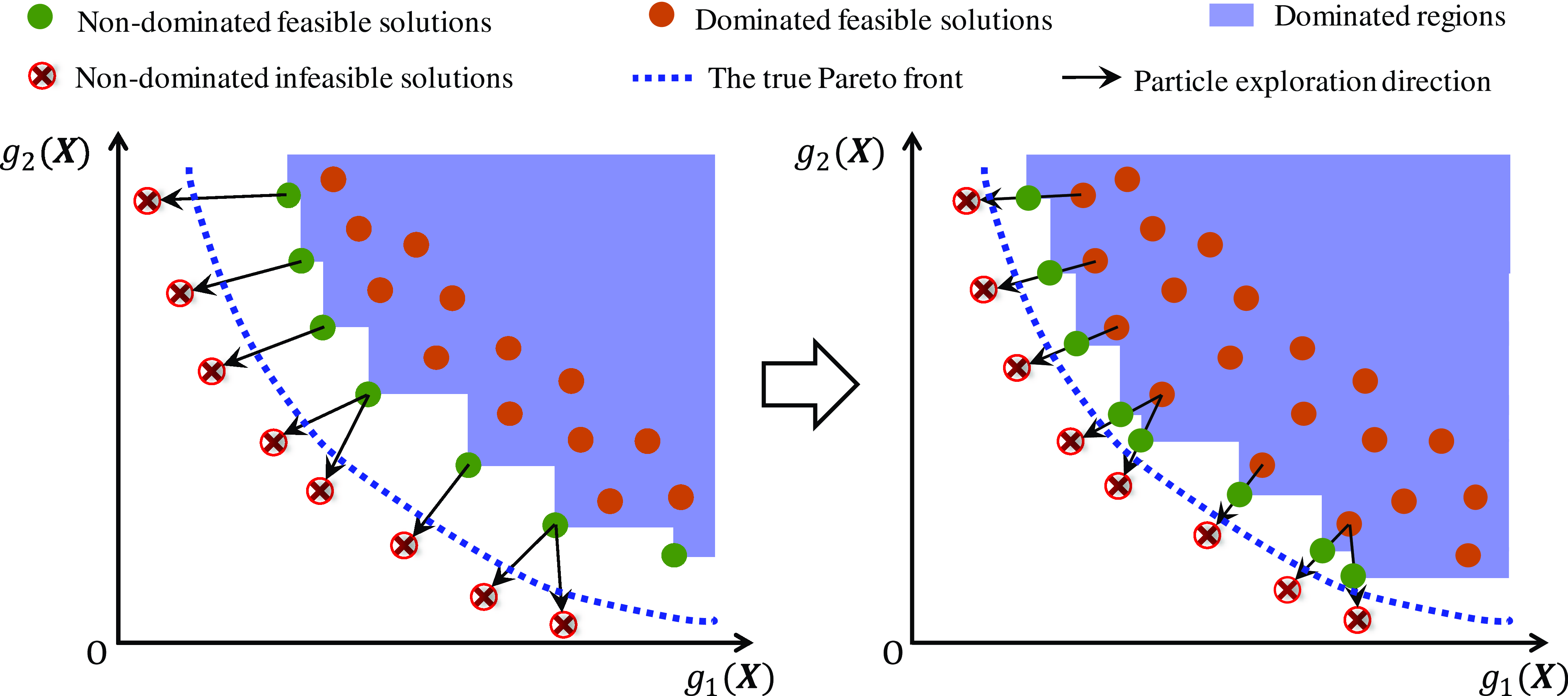
Actually, the decision space is divided into two sets based on whether the constraints are violated: the feasible solution set and the infeasible solution set. These are mapped into the objective space to form two regions: the feasible region and the infeasible region. The true Pareto front serves as the boundary between the feasible and infeasible domains. Therefore, a complementary dual-archive guided boundary exploration strategy is developed in this paper by constructing two complementary external archives: one for storing non-dominated feasible solutions and another for non-dominated infeasible solutions, thereby bridging the feasible and infeasible domains. As shown in Figure 2, the lower left region of the true Pareto front represents the infeasible region, while the upper right region represents the feasible region. In the iterative optimization process of particle swarm optimization, the non-dominated feasible solutions gradually approach the true Pareto front from the direction of the feasible domain, while the non-dominated infeasible solutions approach it from the direction of the infeasible domain. In summary, the complementary dual-archive guided boundary exploration strategy effectively connects the feasible and infeasible regions by leveraging information from infeasible solutions near the constraint boundaries. This approach heuristically guides the particle swarm in exploring regions close to these boundaries, significantly improving the evolutionary optimization capability of the swarm and yielding a greater number of high-quality non-dominated solutions.
Guiding particles to approach constraint boundary by complementary dual archive.

Specifically, let
 $\mathbf{P}_{\mathrm{FS}}$
denote the primary archive storing all non-dominated feasible solutions and
 $\mathbf{P}_{\mathrm{IS}}$
denote the secondary archive storing all non-dominated infeasible solutions. For each infeasible solution
 $\mathbf{P}_{\mathrm{IS}}(j,\colon )$
in the secondary archive, the closest feasible solution
 $\boldsymbol{X}_{\mathrm{FS}}$
in decision space from the primary archive is selected to form a new solution
 $\boldsymbol{X}_{\mathrm{new}}$
between them. If the constraint violation
 $\boldsymbol{F}(\boldsymbol{X}_{\mathrm{new}})$
of
 $\boldsymbol{X}_{\mathrm{new}}$
is non-zero,
 $\mathbf{P}_{\mathrm{IS}}(j,\colon )$
will be replaced by
 $\boldsymbol{X}_{\mathrm{new}}$
, guiding the infeasible solutions towards the constraint boundaries. If
 $\boldsymbol{F}(\boldsymbol{X}_{\mathrm{new}})$
is zero,
 $\boldsymbol{X}_{\mathrm{new}}$
will be added to
 $\mathbf{P}_{\mathrm{FS}}$
, guiding the feasible solutions towards the constraint boundaries. This complementary dual-archive guided boundary expansion process facilitates approaching the constraint boundaries from both feasible and infeasible regions simultaneously, significantly enhancing the optimization efficiency of the particle swarm and yielding a greater number of high-quality non-dominated solutions.
 \begin{align}\boldsymbol{X}_{\boldsymbol{FS}}=\underset{\boldsymbol{l}=\left\{\mathbf{1,2},\ldots, \boldsymbol{M}_{\boldsymbol{PF}}\right\}}{\boldsymbol{Fmin}} \left(\boldsymbol{Dist}\left(\boldsymbol{P}_{\boldsymbol{IS}}\left(\boldsymbol{j},\colon \right),\boldsymbol{P}_{\boldsymbol{FS}}\left(\boldsymbol{l},\colon \right)\right)\right) \end{align}
 \begin{align} \boldsymbol{X}_{\boldsymbol{new}}=\boldsymbol{P}_{\boldsymbol{IS}}\left(\boldsymbol{j},\colon \right)+\left(\boldsymbol{X}_{\boldsymbol{FS}}-\boldsymbol{P}_{\boldsymbol{IS}}\left(\boldsymbol{j},\colon \right)\right)/\boldsymbol{N}_{\boldsymbol{insert}} \end{align}
 \begin{align} \begin{cases} \boldsymbol{P}_{\boldsymbol{IS}}\left(\boldsymbol{j},\colon \right)\Leftarrow \boldsymbol{X}_{\boldsymbol{new}}, \boldsymbol{if}\, \boldsymbol{F}\left(\boldsymbol{X}_{\boldsymbol{new}}\right)\gt \mathbf{0}\\ \boldsymbol{P}_{\boldsymbol{FS}}\Leftarrow \left[\boldsymbol{P}_{\boldsymbol{FS}};\boldsymbol{X}_{\boldsymbol{new}}\right], \boldsymbol{if}\, \boldsymbol{F}\left(\boldsymbol{X}_{\boldsymbol{new}}\right)=\mathbf{0} \end{cases} \end{align}
where
 $M_{PF}$
represents the number of non-dominated feasible solutions in the primary archive.
 $\boldsymbol{F}(\boldsymbol{X})$
calculates the constraint violation function value.
 $N_{\text{insert}}$
denotes the given number of intermediate interpolation points.
 $\underset{l=\{1,2,\ldots, M_{\mathrm{PS}}\}}{\mathbf{Fmin}} (\mathbf{Dist}(\mathbf{P}_{\mathrm{IS}}(j,\colon ),\mathbf{P}_{\mathrm{FS}}(l,\colon )))$
denotes the minimum distance between the
 $j$
-th point in
 $\mathbf{P}_{\mathrm{IS}}$
and all
 $M_{PF}$
points in
 $\mathbf{P}_{\mathrm{FS}}$
.
 $\mathbf{Dist}(\mathbf{P}_{\mathrm{IS}}(j,\colon ),\mathbf{P}_{\mathrm{FS}}(l,\colon ))$
represents the distance between the
 $j$
-th point in
 $\mathbf{P}_{\mathrm{IS}}$
and the
 $l$
-th point in
 $\mathbf{P}_{\mathrm{FS}}$
, which can be calculated as
 \begin{equation} Dist\left(P_{\boldsymbol{IS}}\left(\mathbf{j},\colon \right),P_{\boldsymbol{FS}}\left(\mathbf{l},\colon \right)\right)=\sum\nolimits _{\mathbf{i}=\mathbf{1}}^{\mathbf{N}_{\mathbf{h}}}\left(P_{\boldsymbol{IS}}\left(\mathbf{j},\mathbf{i}\right)-P_{\boldsymbol{FS}}\left(\mathbf{l},\mathbf{i}\right)\right)^{2} \end{equation}
3.3 Swarm optimal position updating strategy based on sparsity sorting
To achieve the Pareto front as evenly distributed and comprehensively covered as possible, it is necessary to quantitatively compare the relative merits of all feasible solutions obtained through exploration. This approach facilitates identifying optimal exploration positions for the population, guiding the particle swarm to prioritize regions where non-dominated feasible solutions are sparsely distributed. Existing optimization algorithms typically rank all non-dominated feasible solutions using crowding distance, setting fixed multiples of nearest neighbor distances at both ends. However, these methods lack adaptability to trends in the distribution of non-dominated feasible solutions. This study considers scenarios where the slopes of lines fitted near multiple non-dominated feasible solutions near the endpoints approach zero, indicating that further exploration along the corresponding cost function directions has nearly reached its limit. At such points, redirecting the particle swarm to focus on these areas is unnecessary, as it would prevent ineffective iterations and reduce computational overhead, thereby enhancing the optimization capability of the particle swarm.
Therefore, this study defines sparsity
 $Q_{\text{spar}}$
to quantify the dispersion of non-dominated feasible solution distributions in the objective space. Sparsity is described quantitatively by the sum of normalized distances between adjacent non-dominated feasible solutions in the objective space, and adaptively characterized by the slopes of lines fitted to
 $N_{\alpha }$
non-dominated feasible solutions near the endpoints. A higher sparsity value of a non-dominated feasible solution indicates a sparser distribution of non-dominated feasible solutions nearby, resulting in a higher ranking. Specifically, all non-dominated feasible solutions
 $[\boldsymbol{X}_{1}^{*},\boldsymbol{X}_{2}^{*},\ldots, \boldsymbol{X}_{M_{PF}}^{*}]$
are first sorted in ascending order along the first cost function dimension
 \begin{equation} \left(\left[\hat{\mathrm{g}}_{\mathbf{1}}\left(\mathbf{1}\right),\hat{\mathrm{g}}_{\mathbf{1}}\left(\mathbf{2}\right),\ldots, \hat{\mathrm{g}}_{\mathbf{1}}\left(\mathbf{M}_{\mathbf{PF}}\right)\right],\mathrm{N}_{\mathbf{g}\mathbf{1}}\right)=\textit{SortAscend}\left(\left[\mathrm{g}_{\mathbf{1}}\left(\mathbf{1}\right),\ldots, \mathrm{g}_{\mathbf{1}}\left(\mathbf{M}_{\mathbf{PF}}\right)\right]\right) \end{equation}
where
 $M_{PF}$
denotes the number of non-dominated feasible solutions in the primary archive. The function
 $\textbf{SortAscnd}(\boldsymbol{B})$
is employed to re-order the elements in array
 $\boldsymbol{B}$
in ascending order. Specifically, given the original array
 $\boldsymbol{g}_{1}=[\boldsymbol{g}_{1}(1),\ldots, \boldsymbol{g}_{1}(M_{PF})]$
, sorting it results in
 $\hat{\boldsymbol{g}}_{1}=[\hat{\boldsymbol{g}}_{1}(1),\ldots, \hat{\boldsymbol{g}}_{1}(M_{PF})]$
such that
 $\hat{\boldsymbol{g}}_{1}(1)\leq \hat{\boldsymbol{g}}_{1}(2)\leq \cdots \leq \hat{\boldsymbol{g}}_{1}(i)\leq \cdots \leq \hat{\boldsymbol{g}}_{1}(M_{PF})$
.
 $\boldsymbol{N}_{g1}$
represents the mapping relationship between the indices of elements in the reordered array
 $\hat{\boldsymbol{g}}_{1}$
and those in the original array
 $\boldsymbol{g}_{1}$
, that is,
 $\hat{\boldsymbol{g}}_{1}(i)=\boldsymbol{g}_{1}(\boldsymbol{N}_{g1}(i))$
.
Subsequently, all non-dominated feasible solutions
 $[\boldsymbol{X}_{1}^{*},\boldsymbol{X}_{2}^{*},\ldots, \boldsymbol{X}_{M_{PF}}^{*}]$
are sorted in descending order based on the second objective function dimension.
 \begin{equation} \left(\left[\hat{\mathrm{g}}_{\mathbf{2}}\left(\mathbf{1}\right),\hat{\mathrm{g}}_{\mathbf{2}}\left(\mathbf{2}\right),\ldots, \hat{\mathrm{g}}_{\mathbf{2}}\left(\mathbf{M}_{\mathbf{PF}}\right)\right],\mathrm{N}_{\mathbf{g}\mathbf{2}}\right)=\boldsymbol{SortDescent}\left(\left[\mathrm{g}_{\mathbf{2}}\left(\mathbf{1}\right),\ldots, \mathrm{g}_{\mathbf{2}}\left(\mathbf{M}_{\mathbf{PF}}\right)\right]\right) \end{equation}
where the function
 $\textbf{SortDescent}(\boldsymbol{C})$
is utilized to reorder elements in array
 $\boldsymbol{C}$
in descending order. Thus, the original array
 $\boldsymbol{g}_{2}=[\boldsymbol{g}_{2}(1),\boldsymbol{g}_{2}(2),\ldots, \boldsymbol{g}_{2}(M_{PF})]$
when sorted in descending order yields the new array
 $\hat{\boldsymbol{g}}_{2}=[\hat{\boldsymbol{g}}_{2}(1),\hat{\boldsymbol{g}}_{2}(2),\ldots, \hat{\boldsymbol{g}}_{2}(M_{PF})]$
, satisfying
 $\hat{\boldsymbol{g}}_{2}(1)\geq \hat{\boldsymbol{g}}_{2}(2)\geq \cdots \geq \hat{\boldsymbol{g}}_{2}(i)\geq \cdots \geq \hat{\boldsymbol{g}}_{2}(M_{PF})$
.
 $\boldsymbol{N}_{g2}$
denotes the mapping between the indices of elements in the reordered array
 $\hat{\boldsymbol{g}}_{2}$
and those in the original array
 $\boldsymbol{g}_{2}$
, specifically
 $\hat{\boldsymbol{g}}_{2}(i)=\boldsymbol{g}_{2}(\boldsymbol{N}_{g2}(i))$
.
Given that the non-dominated feasible solutions do not dominate each other, it follows that
 $\boldsymbol{N}_{g1}(i)=\boldsymbol{N}_{g2}(i)$
. This means that the ascending order index of a non-dominated feasible solution in the time cost function dimension equals its descending order index in the energy cost function dimension. Define the distance between adjacent cost function values as
 \begin{equation} \mathbf{d}_{\mathbf{l},\mathbf{i}}=\frac{\hat{\mathrm{g}}_{\mathbf{l}}\left(\mathbf{i}+\mathbf{1}\right)-\hat{\mathrm{g}}_{\mathbf{l}}\left(\mathbf{i}\right)}{\hat{\mathrm{g}}_{\mathbf{l}}\left(\mathbf{M}_{\mathbf{PF}}\right)-\hat{\mathrm{g}}_{\mathbf{l}}\left(\mathbf{1}\right)}, \mathbf{i}=\mathbf{1,2},\mathbf{3},\ldots, \mathbf{M}_{\mathbf{PF}}-\mathbf{1} \end{equation}
Building upon this foundation, to achieve optimal exploration of the population, strategies are devised to guide the particle swarm towards regions where non-dominated feasible solutions are sparsely distributed. Formulas are defined to calculate the sparsity of non-dominated feasible solutions at different positions.
(1) The formula for calculating the sparsity of the non-dominated feasible solution
 $\boldsymbol{X}_{1}^{*}$
at the initial position is
 \begin{equation} \mathbf{Q}_{\boldsymbol{spar}}\left(\mathbf{N}_{\mathbf{g}\mathbf{1}}\left(\mathbf{1}\right)\right)=\mathbf{\alpha }_{\mathbf{g}\mathbf{1}}\left(\mathbf{d}_{\mathbf{1,1}}+\mathbf{d}_{\mathbf{2,1}}\right)\frac{\left\| \mathrm{X}_{\mathbf{N}_{\mathbf{g}\mathbf{1}}\left(\mathbf{1}\right)}^{\mathbf{*}}-\mathrm{X}_{\boldsymbol{\min }}\right\| }{\left\| \mathrm{X}_{\boldsymbol{\max }}-\mathrm{X}_{\boldsymbol{\min }}\right\| } \end{equation}
where
 $\alpha _{g1}$
denotes the slope of the line fitted to the first
 $N_{\alpha }$
non-dominated feasible solutions at the initial position, calculated as
 \begin{equation} \mathbf{\alpha }_{\mathbf{g}\mathbf{1}}=Atan\left(\frac{\hat{\mathrm{g}}_{\mathbf{2}}\left(\mathbf{M}_{\mathbf{PF}}\right)-\hat{\mathrm{g}}_{\mathbf{2}}\left(\mathbf{1}\right)}{\hat{\mathrm{g}}_{\mathbf{1}}\left(\mathbf{M}_{\mathbf{PF}}\right)-\hat{\mathrm{g}}_{\mathbf{1}}\left(\mathbf{1}\right)}\left(\frac{\mathbf{1}}{\mathbf{N}_{\mathbf{\alpha }}}\sum \nolimits_{\mathbf{j}=\mathbf{1}}^{\mathbf{N}_{\mathbf{\alpha }}}\frac{\hat{\mathrm{g}}_{\mathbf{1}}\left(\mathbf{j}+\mathbf{1}\right)-\hat{\mathrm{g}}_{\mathbf{1}}\left(\mathbf{j}\right)}{\hat{\mathrm{g}}_{\mathbf{2}}\left(\mathbf{j}+\mathbf{1}\right)-\hat{\mathrm{g}}_{\mathbf{2}}\left(\mathbf{j}\right)}\right)\right) \end{equation}
(2) The formula for calculating the sparsity of the non-dominated feasible solution
 $\boldsymbol{X}_{i}^{*}$
at intermediate positions (
 $i=2,3,\ldots, M_{PF}-1$
) is
 \begin{equation} \mathbf{Q}_{\boldsymbol{spar}}\left(\mathbf{N}_{\mathbf{g}\mathbf{1}}\left(\mathbf{i}\right)\right)=\mathbf{d}_{\mathbf{1},\mathbf{i}}+\mathbf{d}_{\mathbf{1},\mathbf{i}-\mathbf{1}}+\mathbf{d}_{\mathbf{2},\mathbf{i}}+\mathbf{d}_{\mathbf{2},\mathbf{i}-\mathbf{1}}, \mathbf{i}=\mathbf{2,3},\ldots, \mathbf{M}_{\mathbf{PF}}-\mathbf{1} \end{equation}
(3) The formula for calculating the sparsity of the non-dominated feasible solution
 $\boldsymbol{X}_{M_{PF}}^{*}$
at the terminal position is
 \begin{equation} \mathbf{Q}_{\boldsymbol{spar}}\left(\mathbf{N}_{\mathbf{g}\mathbf{1}}\left(\mathbf{M}_{\mathbf{PF}}\right)\right)=\mathbf{\alpha }_{\mathbf{g}\mathbf{2}}\left(\mathbf{d}_{\mathbf{1},{\mathbf{M}_{\mathbf{PF}}}-\mathbf{1}}+\mathbf{d}_{\mathbf{2},{\mathbf{M}_{\mathbf{PF}}}-\mathbf{1}}\right)\frac{\left\| \mathrm{X}_{\boldsymbol{\max }}-\mathrm{X}_{\mathbf{N}_{\mathbf{g}\mathbf{1}}\left(\mathbf{M}_{\mathbf{PF}}\right)}^{\mathbf{*}}\right\| }{\left\| \mathrm{X}_{\boldsymbol{\max }}-\mathrm{X}_{\boldsymbol{\min }}\right\| } \end{equation}
where
 $\alpha _{g2}$
denotes the slope of the line fitted to the last
 $N_{\alpha }$
non-dominated feasible solutions at the terminal position, calculated as
 \begin{equation} \mathbf{\alpha }_{\mathbf{g}\mathbf{2}}=Atan\left(\frac{\hat{\mathrm{g}}_{\mathbf{1}}\left(\mathbf{M}_{\mathbf{PF}}\right)-\hat{\mathrm{g}}_{\mathbf{1}}\left(\mathbf{1}\right)}{\hat{\mathrm{g}}_{\mathbf{2}}\left(\mathbf{M}_{\mathbf{PF}}\right)-\hat{\mathrm{g}}_{\mathbf{2}}\left(\mathbf{1}\right)}\left(\frac{\mathbf{1}}{\mathbf{N}_{\mathbf{\alpha }}}\sum _{\mathbf{j}=\mathbf{M}_{\mathbf{PF}}-\mathbf{N}_{\mathbf{\alpha }}}^{\mathbf{M}_{\mathbf{PF}}-\mathbf{1}}\frac{\hat{\mathrm{g}}_{\mathbf{2}}\left(\mathbf{j}+\mathbf{1}\right)-\hat{\mathrm{g}}_{\mathbf{2}}\left(\mathbf{j}\right)}{\hat{\mathrm{g}}_{\mathbf{1}}\left(\mathbf{j}+\mathbf{1}\right)-\hat{\mathrm{g}}_{\mathbf{1}}\left(\mathbf{j}\right)}\right)\right) \end{equation}
When quantitatively comparing the relative merits of all feasible solutions, the first step involves determining the dominance relationships among the multi-dimensional objective vectors corresponding to each feasible solution, thereby eliminating dominated solutions. Subsequently, among all non-dominated feasible solutions, sorting is performed based on sparsity, and the non-dominated feasible solution with the highest current sparsity is selected as the optimal exploration position for the population. This guides the particle swarm to accelerate exploration in regions where non-dominated feasible solutions are currently sparsely distributed, thereby enhancing the uniform distribution and comprehensive coverage of the final Pareto front.
3.4 Trajectory optimization process for manipulators based on HMOPSO
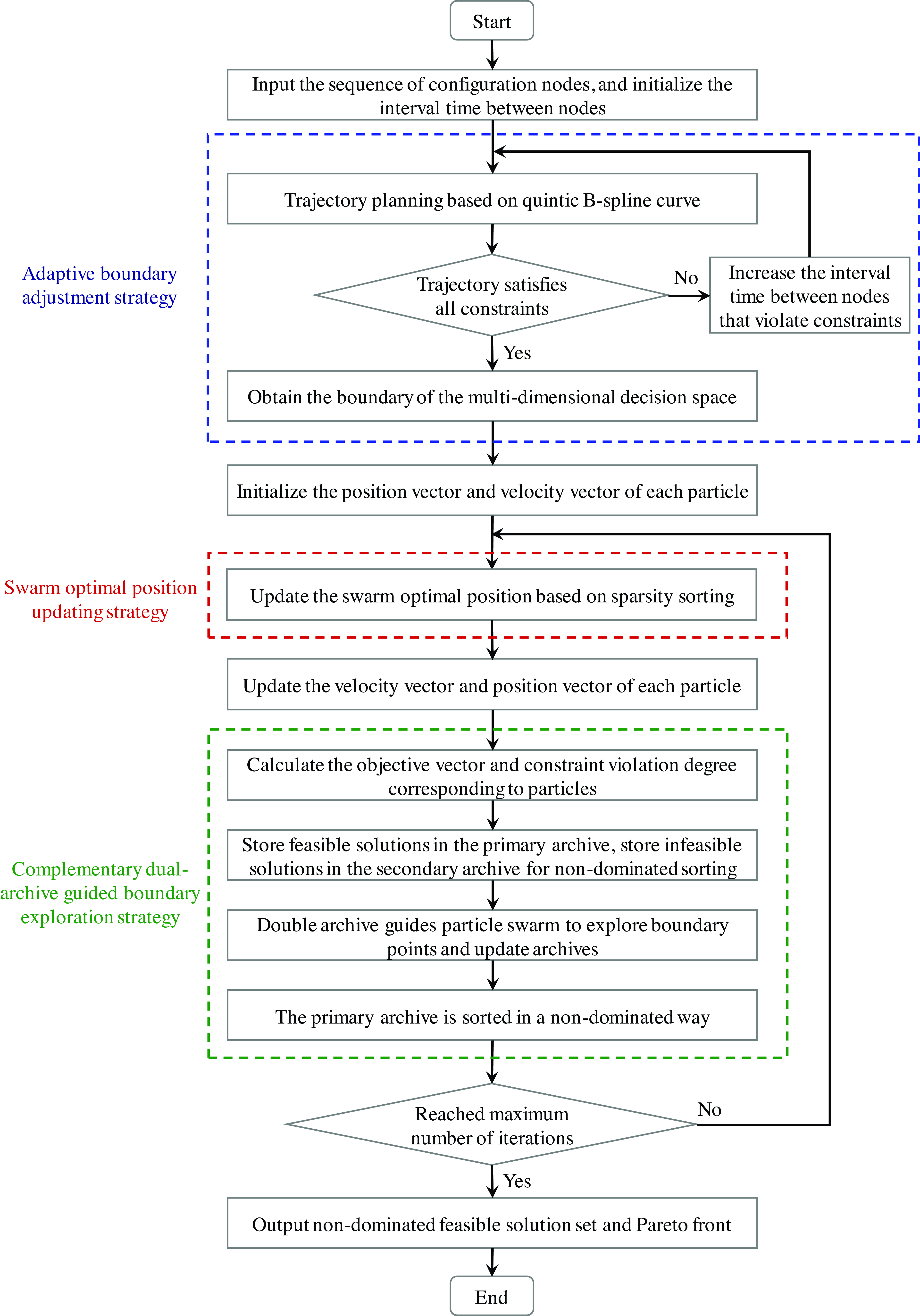
Integrating the previously designed strategies – adaptive boundary adjustment strategy of multi-dimensional decision space, complementary dual-archive guided boundary exploration strategy, and swarm optimal position updating strategy based on sparsity sorting – into the existing MOPSO algorithm results in the heuristic multi-objective particle swarm optimization algorithm (HMOPSO). The trajectory optimization process of a manipulator based on the HMOPSO algorithm is illustrated in the diagram, as shown in Figure 3. The adaptive boundary adjustment strategy is designed to achieve precise adaptation of the multi-dimensional decision space boundaries by specifically regulating the time intervals between adjacent configuration nodes. The complementary dual-archive guided boundary exploration strategy is used for connecting the feasible and infeasible regions by leveraging information from infeasible solutions near the constraint boundaries, thereby heuristically guiding the particle swarm to explore regions close to these boundaries, significantly improving the particle swarm’s evolutionary optimization capability and yielding a greater number of high-quality non-dominated solutions. The swarm optimal position updating strategy based on sparsity sorting is designed to guide the particle swarm toward areas on the Pareto front where non-dominated solutions are sparsely distributed, ensuring the uniformity and completeness of the final Pareto front.
Flow chart of trajectory optimization for manipulators based on HMOPSO.

Algorithm : TrajectoryOptimizationViaHMOPSO (\Pi path)

4. Experiment design and experimental results discussion
To evaluate the feasibility and superiority of the proposed HMOPSO algorithm for energy-efficient trajectory optimization of manipulators, this section compares HMOPSO with five existing advanced algorithms in the field of multi-objective optimization. The performance of each algorithm in the trajectory optimization task for planetary surface manipulators is assessed through metrics such as the inverse generational distance and the dominant area. All experiments were performed on a desktop computer equipped with Windows 10 environment and an Intel Core i7-8700K processor with the main frequency of 3.7 GHz and the memory of 24.0 GB.
4.1 Experimental design of manipulator trajectory optimization
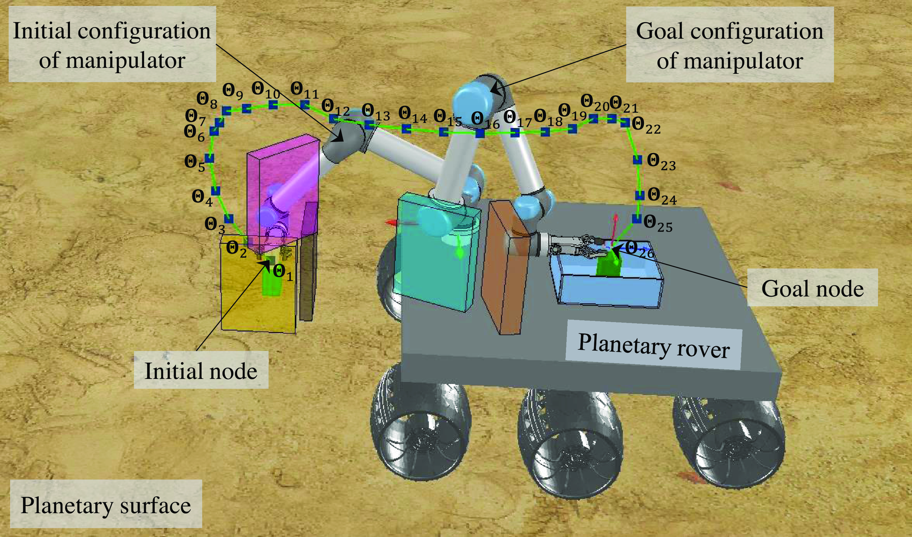
This section presents a scenario for the task of object grasping and transfer using a manipulator, as illustrated in Figure 4. Based on a previously developed robust safety path optimization method [Reference Xiao, Zhang, Wu, Han, Ding and Han31, Reference Xiao, Wu, Weng, Zhang, Han, Dong and Liang32], a path composed of a series of discrete nodes, denoted as
 $\mathbf{\Pi }_{\text{path}}=[\mathbf{\Theta }_{1}, \mathbf{\Theta }_{2},\ldots, \mathbf{\Theta }_{N}]$
, is generated. The proposed optimization algorithm, HMOPSO, along with several advanced algorithms in the field of multi-objective optimization, including NSGA-II, TVMOPSO, NSWOA, SPEA-II, and MOGWO, is employed for the smooth trajectory planning and iterative optimization of the path
 $\mathbf{\Pi }_{\text{path}}$
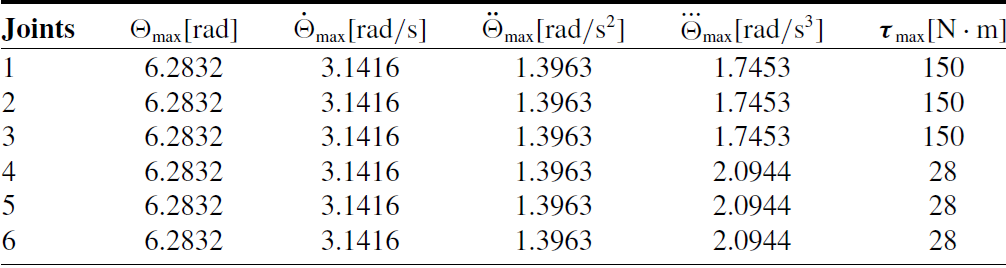
. The aim is to achieve a manipulator trajectory that simultaneously satisfies constraints on joint angular displacement, angular velocity, angular acceleration, angular jerk, and joint torque, while optimizing trajectory duration and energy consumption. The constraints on joint states are presented in Table I. To ensure the fairness and reliability of the performance comparison among the algorithms, all experimental setups and common parameters are kept consistent.
Kinematic and dynamic constraints of each joint of manipulator.

Manipulator operation task scenario and position points corresponding to path nodes.

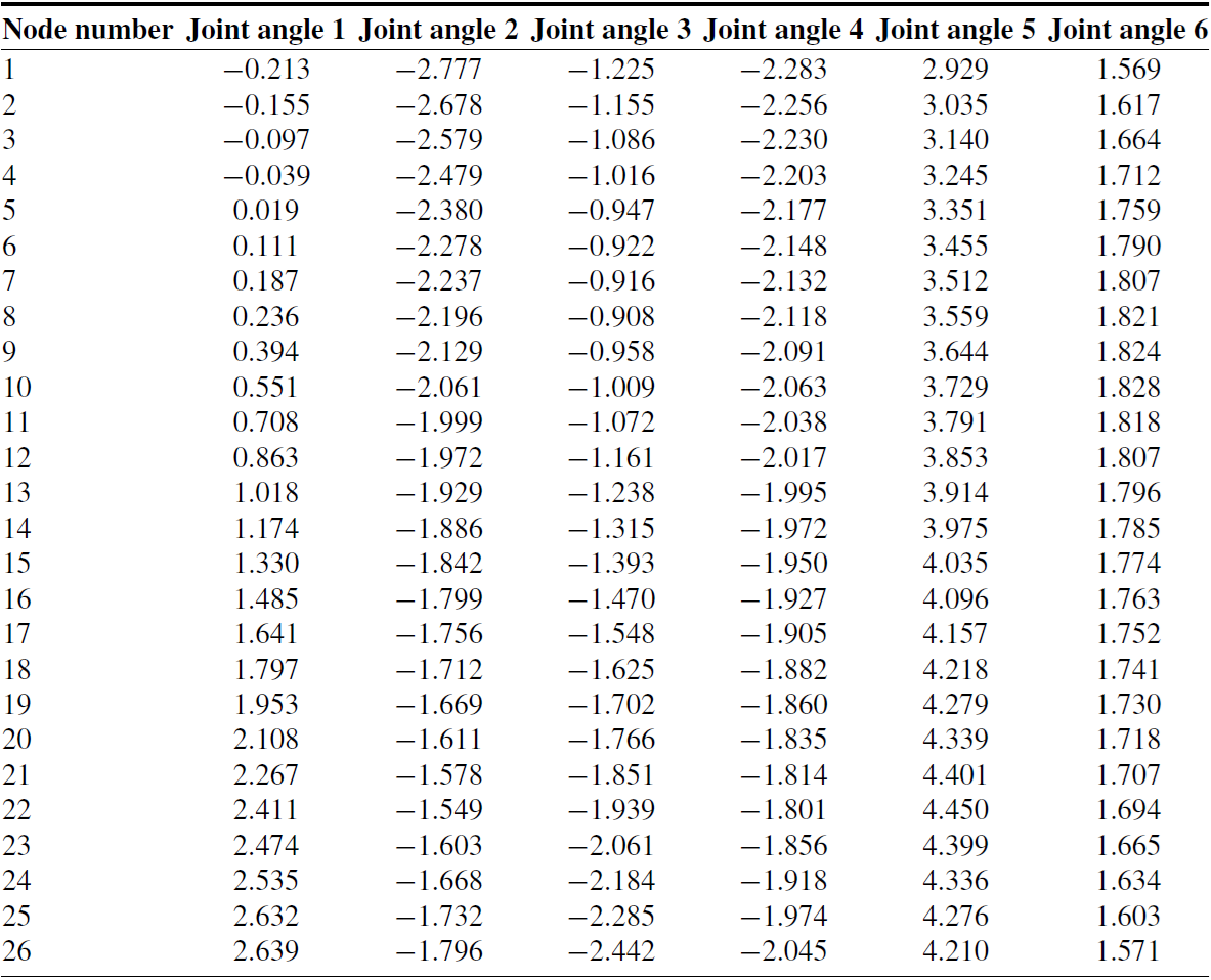
Node sequence of
 $\boldsymbol{\Pi }_{path}$
and its corresponding manipulator joint configuration.

The path
 $\mathbf{\Pi }_{\text{path}}$
consists of 26 discrete nodes, with the node sequence and corresponding manipulator configurations detailed in Table II. The first node represents the initial node, while the last node indicates the goal node. The illustrated figure displays the sequence of positions in the Cartesian space of the manipulator’s end effector, corresponding to the joint configuration parameters at each path node.
4.2 Experimental result discussions
This section focuses on the trajectory planning and iterative optimization of the path
 $\mathbf{\Pi }_{\text{path}}$
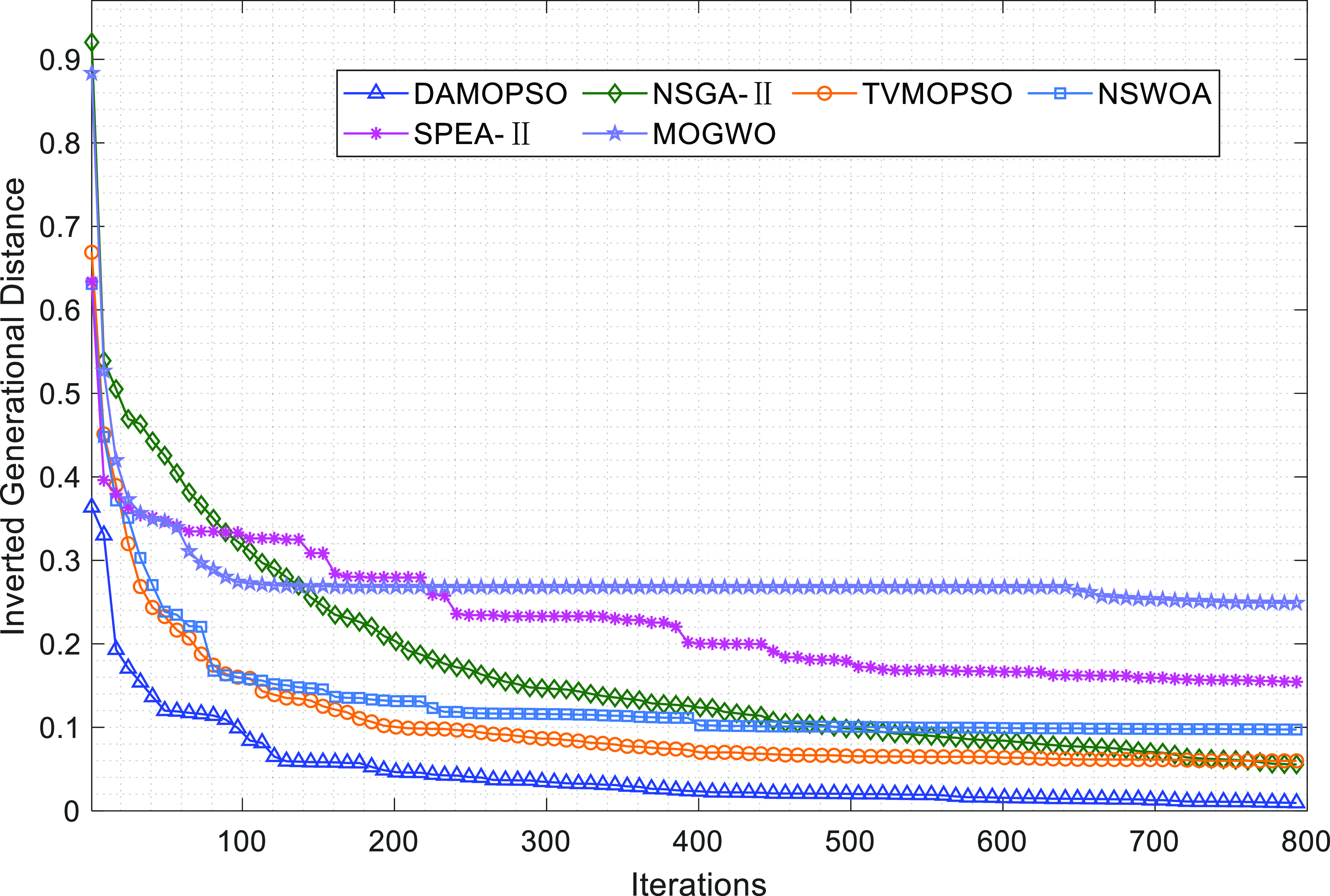
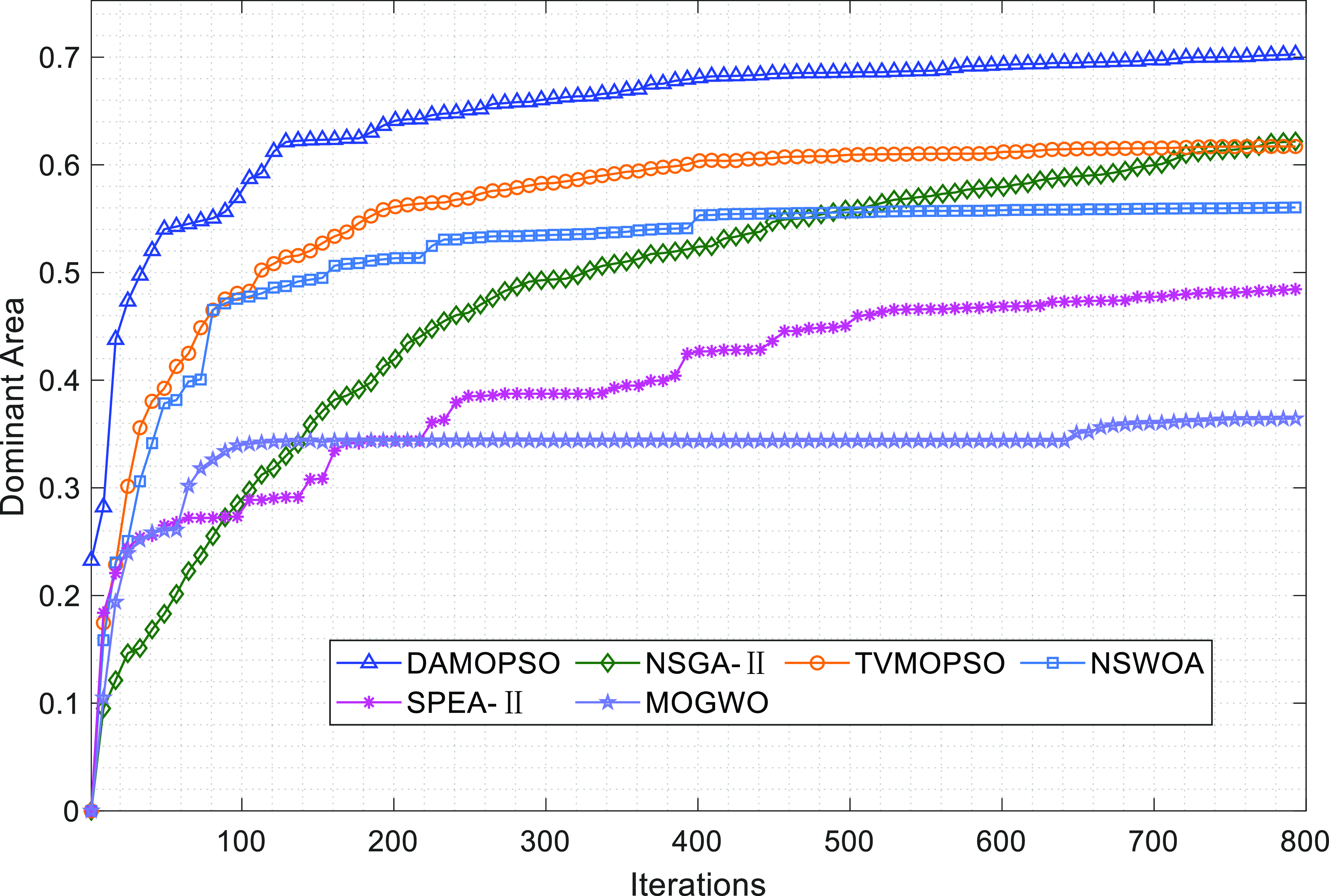
using the developed multi-objective trajectory optimization algorithm HMOPSO, as well as several advanced algorithms in the field of multi-objective optimization, including NSGA-II, TVMOPSO, NSWOA, SPEA-II, and MOGWO. Each algorithm was subjected to 800 iterations, during which Pareto front data were recorded for each optimization process. Subsequently, the Pareto front data obtained from these experiments were analyzed based on performance indicators, including inverse generational distance, dominant area, and utopian optimal solutions, as developed in the previous section. The evolution of inverse generational distance
 $I_{IGD}$
and dominant area
 $I_{DA}$
with respect to iteration count is illustrated in Figs. 5 and 6. Additionally, the final Pareto front achieved by each optimization algorithm are presented in Figure 7. Finally, a comparative analysis of the optimization algorithms is conducted based on the experimental data, evaluating their performance in multi-objective trajectory optimization tasks for the manipulator from the perspectives of inverse generational distance, dominant area, and utopian optimal solutions.
Evolution curve of inverse generation distance
 $I_{IGD}$
during algorithm iteration.

Evolution curve of dominant area
 $I_{DA}$
during algorithm iteration.

Pareto front obtained after 800 iterations of each optimization algorithm.

The inverse generational distance metric
 $I_{IGD}$
is employed to characterize the uniformity of the distribution of the Pareto front
 $\boldsymbol{PF}$
obtained by the algorithms during the experiments and its proximity to the true optimal Pareto front
 $\boldsymbol{PF}^{\# }$
. This study quantifies
 $I_{IGD}$
as the average of the minimum distances between all reference points on the true optimal
 $\boldsymbol{PF}^{\# }$
and the dominated regions of points on the experimental
 $\boldsymbol{PF}$
. The value of
 $I_{IGD}$
ranges from
 $[0,1]$
, with smaller values indicating that the
 $\boldsymbol{PF}$
obtained by the algorithms converges more closely to the true optimal
 $\boldsymbol{PF}^{\# }$
, thus suggesting superior convergence and diversity performance.
In the iterative optimization process of particle swarm optimization, the non-dominated feasible solutions gradually approach the true Pareto front from the direction of the feasible domain, while the non-dominated infeasible solutions approach it from the direction of the infeasible domain. In summary, the complementary dual-archive guided boundary exploration strategy effectively connects the feasible and infeasible regions by leveraging information from infeasible solutions near the constraint boundaries. This approach heuristically guides the particle swarm in exploring regions close to these boundaries, significantly improving the evolutionary optimization capability of the swarm and yielding a greater number of high-quality non-dominated solutions. As illustrated in Figure 5, the evolution of
 $I_{IGD}$
for each algorithm demonstrates a reduction as the number of iterations increases, indicating that all algorithms progressively approach the true optimal Pareto front
 $\boldsymbol{PF}^{\# }$
. Notably, the
 $I_{IGD}$
of the proposed HMOPSO algorithm is consistently lower than that of the other algorithms throughout the iterations. This indicates that the
 $\boldsymbol{PF}$
derived from the HMOPSO algorithm remains closest to the true optimal
 $\boldsymbol{PF}^{\# }$
, reflecting its superior convergence speed and distribution breadth. The success of the HMOPSO algorithm can be attributed to the complementary dual-archive guiding boundary expansion strategy. By constructing two external archives – one for storing non-dominated feasible solutions and the other for non-dominated infeasible solutions – this approach effectively bridges the feasible and infeasible regions. This strategy leverages information from infeasible solutions near the constraint boundaries, guiding the particle swarm to efficiently explore areas close to these boundaries and significantly enhancing the optimization capabilities of the swarm.
The dominant area metric
 $I_{DA}$
quantifies the total area covered by the Pareto front
 $\boldsymbol{PF}$
obtained by the algorithm within the normalized objective space. This metric effectively reflects both the convergence and distribution breadth of the non-dominated feasible solution set. The value of
 $I_{DA}$
ranges from
 $[0,1]$
, with larger values indicating that the
 $\boldsymbol{PF}$
is closer to the true optimal Pareto front
 $\boldsymbol{PF}^{\# }$
, signifying better convergence performance and distribution diversity.
As shown in the evolution curves of
 $I_{DA}$
for various algorithms in Figure 6, the initial
 $I_{DA}$
values for NSGA-II, NSWOA, SPEA-II, and MOGWO are relatively low, while the proposed HMOPSO algorithm exhibits a significantly higher
 $I_{DA}$
value from the outset. This advantage is attributed to the adaptive boundary adjustment strategy for the multi-dimensional decision space and the optimization of the initial positions of the particle swarm. The adaptive adjustment is achieved by precisely controlling the time intervals between adjacent points, thus avoiding inefficient exploration due to excessively large decision space. Additionally, the initial positions of the particles are distributed linearly and uniformly to address the potential relationship between minimizing trajectory duration and energy consumption. This approach maintains diversity within the particle swarm and mitigates the inefficiencies typically associated with traditional optimization algorithms in their early iterations, enabling the swarm to identify numerous high-quality solutions promptly and significantly enhancing optimization efficiency. Moreover, the
 $I_{DA}$
of the HMOPSO algorithm consistently exceeds that of the other algorithms throughout the iterations, indicating that the non-dominated feasible solution set corresponding to its
 $\boldsymbol{PF}$
remains superior. This suggests that the HMOPSO algorithm outperforms others in terms of both convergence speed and precision.
Performance index data calculated after 800 iterations of each optimization algorithm.

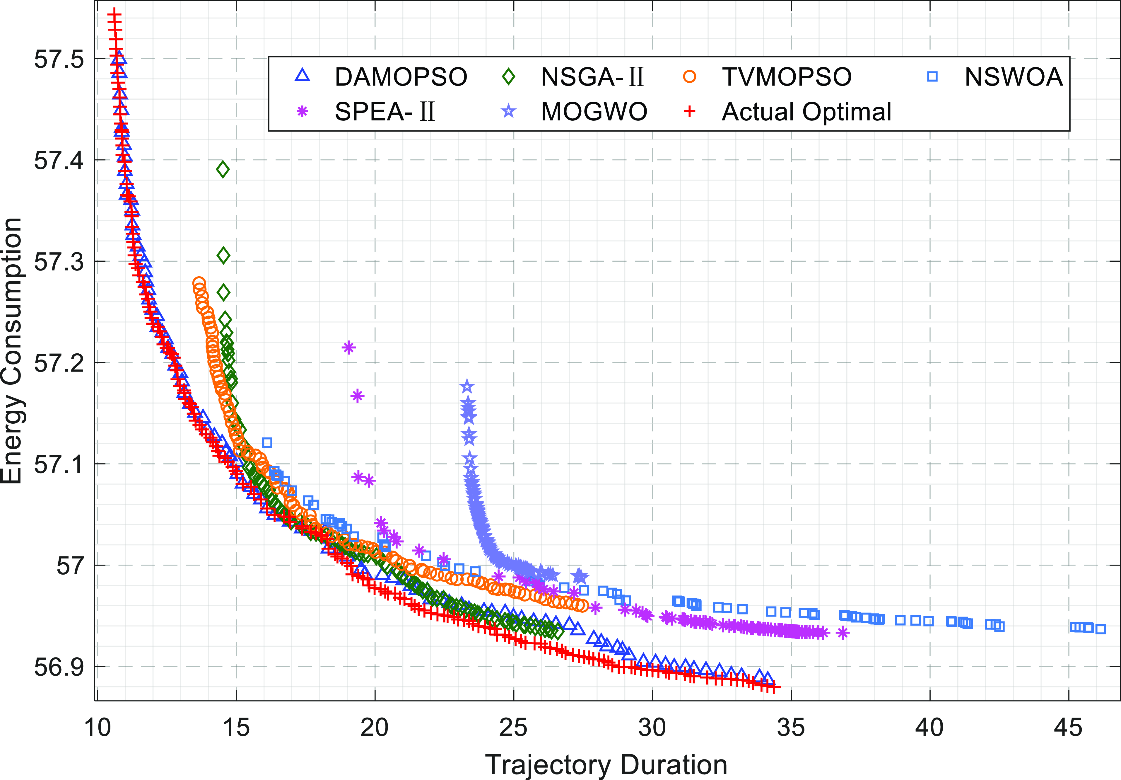
Furthermore, Figure 7 illustrates the final Pareto front obtained after 800 iterations of various optimization algorithms. The Pareto front from NSWOA, SPEA-II, and MOGWO are relatively distant from the true optimal Pareto front
 $\boldsymbol{PF}^{\# }$
, while the non-dominated solutions on the Pareto front from NSGA-II and TVMOPSO exhibit lower quality in terms of minimizing trajectory duration. In contrast, the HMOPSO algorithm proposed in this study yields Pareto front that closely approximate the true optimal Pareto front
 $\boldsymbol{PF}^{\# }$
. Additionally, the non-dominated solutions on its Pareto front show wider coverage and more uniform distribution. Such proximity to optimality, extensive coverage, and uniform distribution suggests that the HMOPSO algorithm can provide a greater number of high-quality non-dominated solutions. This is crucial for decision-makers who need to select a set of optimal trajectory parameter solutions from the relatively uniformly distributed non-dominated solutions along the Pareto front for subsequent trajectory generation.
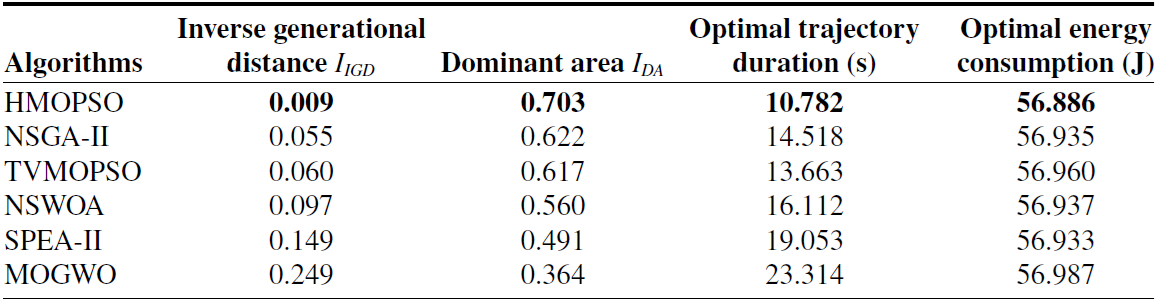
According to the performance metrics obtained after 800 iterations of various optimization algorithms, it is evident from Table III that the MOGWO algorithm yields the worst optimal trajectory duration (23.314 s), while the HMOPSO algorithm developed in this study significantly outperforms others with an optimal trajectory duration of 10.782 s. This improvement is attributed to the existing algorithms employing a single external archive that only includes feasible solutions that meet constraints, discarding infeasible solutions directly. However, infeasible solutions, especially those near the constraint boundaries, contain critical information and can sometimes be closer to the true optimal Pareto front than feasible solutions stored in the archive. Therefore, the HMOPSO algorithm incorporates two external archives: a primary archive for storing non-dominated feasible solutions and a secondary archive for non-dominated infeasible solutions. This dual-archive approach connects the feasible and infeasible regions, effectively utilizing the information from infeasible solutions near the constraint boundaries. Consequently, this guides the particle swarm to efficiently explore and approach optimal solutions within these critical areas, resulting in the identification of high-quality solutions with reduced trajectory durations.
This section highlights the superiority of the HMOPSO algorithm developed in this study compared to existing optimization algorithms. An experimental setup was established where each algorithm iterated 800 times, allowing for a comparative analysis of the performance evolution curves across all algorithms. During the trajectory optimization tasks for planetary surface manipulators, decision-makers can flexibly adjust the number of iterations based on specific needs and field conditions to obtain the Pareto front within an appropriate timeframe. From the performance evolution curves and previous experimental results, it is evident that reducing the number of iterations leads to a decline in the quality of the Pareto front across all algorithms; however, the HMOPSO algorithm consistently outperforms NSGA-II, TVMOPSO, NSWOA, SPEA-II, and MOGWO.
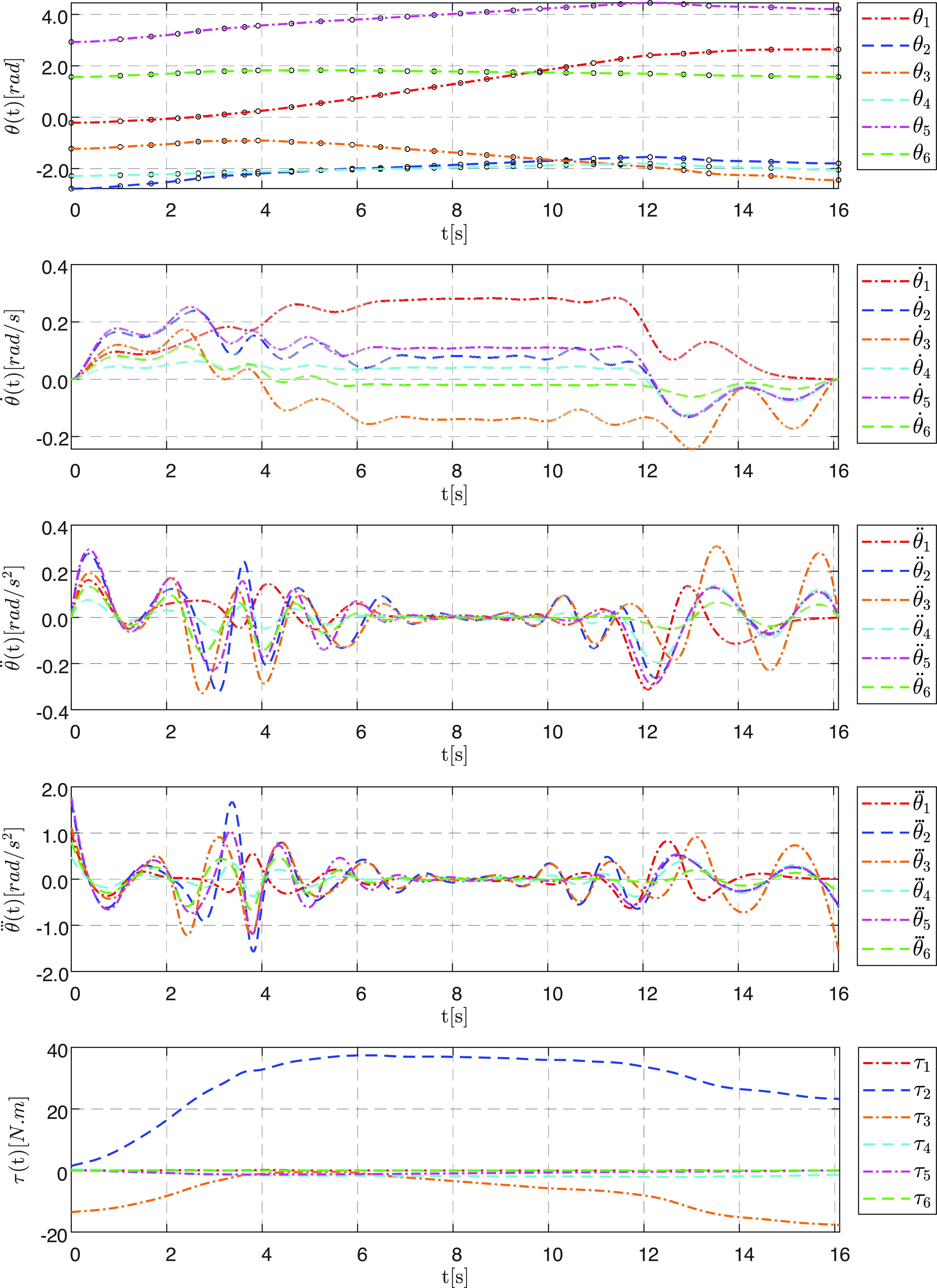
Motion state curves of the joints generated based on the comprehensive optimal solution.

Configuration state of the manipulator in moving along optimized trajectory.

This advantage can be attributed to the adaptive boundary adjustment strategy for the multi-dimensional decision space, the complementary dual-archive guided boundary exploration strategy, and the swarm optimal position updating strategy based on sparsity sorting. In multi-objective trajectory parameter optimization experiments focusing on trajectory fitting, minimizing duration, and reducing energy consumption, the HMOPSO algorithm demonstrates enhanced evolutionary optimization capabilities and faster convergence rates. The resulting Pareto front closely approximates the true optimal Pareto front, with a broader coverage and more uniform distribution of non-dominated solutions. Additionally, performance metrics such as the inverted generation distance and dominant area during the iterative optimization process of the HMOPSO algorithm significantly exceed those of existing multi-objective optimization algorithms.
4.3 Generating energy-efficient trajectory for manipulator
After obtaining the non-dominated feasible solution set
 $\mathbf{\Omega }_{{X^{\boldsymbol{*}}}}$
and its corresponding Pareto front
 $\boldsymbol{PF}$
in multi-objective optimization, the manipulator decision-maker can discern the interdependencies among the cost functions. During actual operational tasks, planetary surface manipulators can select a specific point from the Pareto front
 $\boldsymbol{PF}$
as the optimal solution, based on the current energy supply and time constraints, along with overall task requirements and pre-defined preferences. This chosen optimal point corresponds to a non-dominated feasible solution, resulting in a motion trajectory that satisfies all constraints while achieving multi-objective optimization. This section utilizes the Pareto front derived from the HMOPSO algorithm to select a set of solutions that optimally balances trajectory duration and energy consumption. A trajectory planning method based on quintic B-spline curves is employed to construct the node vector and calculate control points, thereby generating smooth and energy-efficient motion trajectories for the manipulator’s joints, as illustrated in Figure 8. As shown in Table I, the motion state parameters of the manipulator’s joints consistently adhere to the specified constraints, including joint angular displacement, joint angular velocity, joint angular acceleration, and joint torque throughout the trajectory. Finally, the planned motion reference trajectory is transmitted to the manipulator joint controller to ensure that each joint accurately follows the reference trajectory, enabling the manipulator to efficiently complete the operational tasks. The configuration states of the manipulator at various moments along the optimized trajectory are depicted in Figure 9.
5. Conclusions and future work
This paper proposed an energy-efficient trajectory optimization algorithm named HMOPSO for planetary surface manipulators under kinematic and dynamic constraints. An adaptive boundary adjustment strategy for the multi-dimensional decision space is proposed, which enables precise adaptation of the decision space boundaries by adjusting the time intervals between neighboring configuration nodes. Existing algorithms often discard infeasible solutions that violate constraints during the iterative exploration process. However, infeasible solutions near the constraint boundaries can provide crucial information and may be closer to the true optimal Pareto front than feasible solutions in the archive. To address this, two external archives are constructed: a primary archive for storing non-dominated feasible solutions and a secondary archive for non-dominated infeasible solutions. This approach connects the feasible and infeasible regions, allowing the particle swarm to efficiently explore areas near the constraint boundaries, thereby enhancing its evolutionary optimization capability. Additionally, a swarm optimal position updating strategy based on sparsity sorting is designed to guide the particle swarm toward exploring positions where non-dominated solutions on the Pareto front are more sparsely distributed. This ensures uniformity and completeness in the final Pareto front. The HMOPSO algorithm, incorporating these improvements, is compared with existing advanced algorithms in the field of multi-objective optimization for trajectory optimization tasks involving manipulators. Experimental results demonstrate that the HMOPSO algorithm exhibits superior evolutionary optimization capabilities and faster convergence rates. The final Pareto front obtained closely approximates the true optimal Pareto front, with a broader and more uniform distribution of non-dominated solutions. Moreover, performance metrics such as inverse generation distance and dominant area during the iterative process of HMOPSO significantly outperform those of existing optimization algorithms.
To apply the proposed algorithm to the real-world tasks of planetary surface manipulators, further research is necessary in the following areas: (1) Development of intelligent environmental perception and localization methods to rapidly detect the distribution of obstacles in the operational environment, accurately establish the initial and goal poses of the manipulator, and provide timely environmental information for motion planning, (2) construction of a dynamic surrogate model for the manipulator that achieves a balance between high precision and low complexity, thereby minimizing the time cost associated with the computation of the energy cost function and joint torque constraints during trajectory parameter optimization, (3) establishment of a highly realistic research base for planetary surface construction and operation tasks, where the designed motion planning methods can be deployed on physical manipulators to conduct experimental validations of tasks such as soil collection, equipment assembly, and facility maintenance.
Author contributions
All authors contributed to the study conception and design. Initial material preparation and analysis were performed by Guangzhou Xiao. Yuting Ma carried out the experiments and conducted data gathering. Yunpeng Li performed data analysis. The first draft of the manuscript was written by Guangzhou Xiao. All authors commented on previous versions of the manuscript.
Financial support
This work was partially supported by National Natural Science Foundation of China (62225305, 62003117).
Competing interests
The authors declare no conflicts of interest exist.
Ethical approval
Not applicable.