2.1 Governing equations

The sphere and the two immiscible fluids form a three-phase system. The evolution of this system is described within the framework of a one-fluid approach coupled with an immersed boundary method (IBM). To this end, the local fluid medium is considered as a mixture of the two Newtonian pure fluids. It may be characterized by the local volume fraction $C$ of the upper fluid and by density and viscosity fields which depend only on $C$ and on the intrinsic physical properties of each pure fluid. The volume fraction $C$ obeys the hyperbolic transport equation

and the local density and viscosity of the mixture are respectively given by

where indices 1 and 2 refer to the upper and lower fluids, respectively.

The flow is assumed to be incompressible and is characterized by a single velocity field $\boldsymbol{U}$ and a pressure field $P$ throughout the mixture. The governing equations, applied throughout the fluid and solid domains, are given by

where $\boldsymbol{F}_{\unicode[STIX]{x1D6FE}}$ is the capillary force per unit volume, $\boldsymbol{F}_{\boldsymbol{I}\boldsymbol{B}\boldsymbol{M}}$ is an additional force density introduced to take into account the presence of the sphere in the way described below and $\boldsymbol{g}$ denotes gravity. The capillary force is computed using the continuum surface force model designed by Brackbill, Kothe & Zemach (Reference Brackbill, Kothe and Zemach1992), namely

where $\unicode[STIX]{x1D6FE}$ is the interfacial tension which we assume to be uniform.

The IBM approach (Mittal & Iaccarino Reference Mittal and Iaccarino2005; Prosperetti & Tryggvason Reference Prosperetti and Tryggvason2007) employed to account for the presence of the moving sphere is of the body-force type (Yuki, Takeuchi & Kajishima Reference Yuki, Takeuchi and Kajishima2007). That is, the force density $\boldsymbol{F}_{\boldsymbol{I}\boldsymbol{B}\boldsymbol{M}}$ is chosen in the form

where $\boldsymbol{U}_{\boldsymbol{D}}$ is the desired velocity assigned to the medium at the considered location and $\unicode[STIX]{x1D70F}$ denotes a characteristic time which in computational practice coincides with the time step $\unicode[STIX]{x0394}t$ . The volume fraction $\unicode[STIX]{x1D6FC}$ equals 1 in the solid and 0 in the free fluid. Within the solid, $\boldsymbol{U}_{\boldsymbol{D}}$ is set to $\boldsymbol{V}+\unicode[STIX]{x1D734}\times \boldsymbol{r}$ , where $\boldsymbol{V}$ and $\unicode[STIX]{x1D734}$ are the translational and rotational body velocities, respectively, and $\boldsymbol{r}$ is the local distance to the body centre of inertia. As $\unicode[STIX]{x1D70F}$ goes to zero, any difference between the fluid and body velocities tends to generate an infinite force density at locations where $\unicode[STIX]{x1D6FC}\neq 0$ , thus enforcing the no-slip condition.

The sphere moves according to Newton’s second law. For a rigid body of volume ${\mathcal{V}}$ and density $\unicode[STIX]{x1D70C}_{p}$ , the corresponding overall momentum balance is given by

where $\unicode[STIX]{x1D72E}=-P\boldsymbol{I}+\unicode[STIX]{x1D707}(\unicode[STIX]{x1D735}\boldsymbol{U}+^{\text{T}}\unicode[STIX]{x1D735}\boldsymbol{U})$ is the stress tensor and $\boldsymbol{n}$ is the local unit normal to the body surface ${\mathcal{S}}$ , $\unicode[STIX]{x1D644}$ denoting the unit tensor. In general the torque balance is required to determine the rotation rate $\unicode[STIX]{x1D734}$ . However we shall only consider axisymmetric situations, so that no such rotation exists, making (2.7) sufficient to predict the sphere motion.

Finally, it is important to recall that the experimental tests reported in § 2 of PM1 provide evidence that silicone oil always wets the sphere surface entirely. Hence no contact line exists, so that no contact angle model is introduced in the computational approach.

2.2 Numerical techniques and grid characteristics

Computations are carried out with the JADIM code developed in our team. This code makes use of a finite volume discretization combined with a third-order Runge–Kutta Crank–Nicolson time-advancement algorithm. Centred schemes are used to evaluate the various spatial derivatives in (2.4). Incompressibility is enforced at the end of the complete time step through a projection technique (Calmet & Magnaudet Reference Calmet and Magnaudet1997). The corresponding solutions of the Navier–Stokes equations are second-order accurate in both time and space. The solution of (2.1) is based on a flux corrected transport technique split along each grid direction, as described in Bonometti & Magnaudet (Reference Bonometti and Magnaudet2007). This algorithm provides solutions for the volume fraction $C$ with first-order accuracy in time. No explicit interface reconstruction is carried out after the $C$ distribution is computed, so that the interface may be regarded as ‘diffuse’ in this approach. For this reason, the interfacial layer where $0<C<1$ may not keep a strictly constant thickness, becoming thicker (respectively thinner) in regions where the surrounding flow tends to move apart (respectively compress) the iso- $C$ lines. An example of this behaviour may be seen in figure 1(g–h), where the iso- $C$ contours are almost superimposed along the bottom half of the sphere while some spreading is visible along the meniscus surface. With this ‘diffuse’ approach, no specific procedure or criterion is required to capture the breakup of a fluid thread or drop. Here, such a topological change is simply a ‘through’ with $C\approx 0$ in between two fluid regions where $C\approx 1$ or vice versa. As the transition from $C\approx 0$ to $C\approx 1$ is achieved within 2–3 grid cells, observing such an event typically requires the two ‘plateaus’ where $C\approx 1$ to be separated by 4–6 cells. Details about the evaluation of each term in the governing equations and implementation of the various algorithms may be found in the above two references. The performances of this code in situations approaching those on which we focus here may be appreciated in the study of Bonhomme et al. (Reference Bonhomme, Magnaudet, Duval and Piar2012), where the dynamics of air bubbles crossing an interface between two immiscible liquids was considered. Few computational studies have been carried out so far on approaching three-phase problems. One may mention the work by Blanchette & Shapiro (Reference Blanchette and Shapiro2012) who considered the settling of nearly spherical drops across a two-layer arrangement of miscible fluids with identical viscosities.

Compared to the aforementioned studies, the novelty here is that we need to account for the presence of a rigid body and its interaction with the interface. As we treat the two-phase flow on a fixed grid through the volume of fluid approach, it is natural to deal with the body using the IBM technique which does not require the grid to deform with the body motion. The initial IBM approach implemented in the JADIM code is extensively described in Bigot et al. (Reference Bigot, Bonometti, Lacaze and Thual2014). In this approach, equation (2.7) is solved using the technique proposed by Uhlmann (Reference Uhlmann2005), i.e. the surface integral $\int _{{\mathcal{S}}}\unicode[STIX]{x1D72E}\boldsymbol{\cdot }\boldsymbol{n}\,\text{d}S$ , whose evaluation is complex, is replaced by $\unicode[STIX]{x1D70C}{\mathcal{V}}(\text{d}\boldsymbol{V}/\text{d}t-\boldsymbol{g})-\int _{{\mathcal{V}}}\boldsymbol{F}_{\boldsymbol{I}\boldsymbol{B}\boldsymbol{M}}\,\text{d}V$ which is much simpler to compute. Nevertheless, preliminary tests revealed that several improvements beyond the implementation described by Bigot et al. (Reference Bigot, Bonometti, Lacaze and Thual2014) were desirable. A detailed presentation of these changes may be found in Pierson (Reference Pierson2015); we summarize them in appendix A.

The axisymmetric computations whose results are discussed below were performed in a cylindrical domain with a minimum radius of $12R$ ( $R$ is the sphere radius) and a length which depends on the case under consideration, especially on the time period over which we wish to observe the dynamics of the tail towed by the sphere; this length ranges typically from $18R$ to $30R$ . The interface is usually located initially $12R$ from the top of the domain. The grid is uniform in the vertical direction, $z$ , with typically 50 cells per sphere radius. In the radial direction, $r$ , 200 cells are generally distributed uniformly in the central region, $0<r\leqslant 4R$ , so as to properly describe the boundary layer and the film that surround the sphere over a wide range of conditions; this grid density (as well as that in the $z$ direction) is doubled in the most inertial cases for which small-scale phenomena are expected, as well as in situations where film drainage is expected to play an important role. In the outer region, $r>4R$ , the grid is non-uniform, with cells distributed following an arithmetic law. In appendix A, numerical predictions are compared with experimental data describing the settling of a sphere in a homogeneous fluid up to a Reynolds number $Re_{T}\approx 20$ (based on the sphere radius and terminal velocity). Very good agreement is obtained with the improved IBM technique, provided the grid comprises a minimum of 20 cells per sphere radius. We checked that the boundary layer is properly described when it contains 4–5 cells. Since its thickness is of $O(RRe_{T}^{-1/2})$ , we are confident that the selected grid distribution with 50 cells per sphere radius provides accurate predictions up to Reynolds numbers in the range $100\lesssim Re_{T}\lesssim 150$ , i.e. at least up to the critical Reynolds number $Re_{c}$ at which the axisymmetric flow past a freely falling sphere becomes unstable, $Re_{c}\approx 103$ , as determined by Fabre, Tchoufag & Magnaudet (Reference Fabre, Tchoufag and Magnaudet2012).

3.1 A quasi-static detachment situation

We first consider the early evolution of the flow past a 14 mm diameter polyacetal sphere settling in the V500/water–glycerine pair of fluids (configuration $7b$ in figure 3 of PM1). The associated dimensionless parameters are $Ar=2.2$ , $Bo=3.65$ , $\unicode[STIX]{x1D706}=0.17$ , $\unicode[STIX]{x1D701}=0.24$ and $\unicode[STIX]{x1D701}_{p}=0.40$ .

Figure 1.

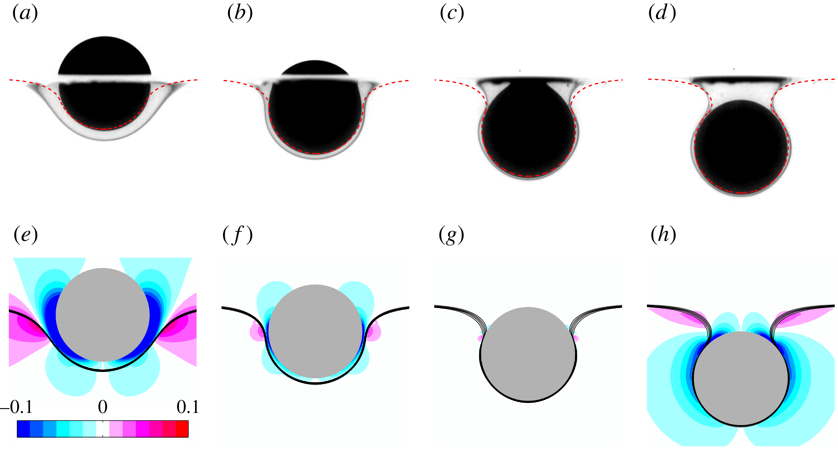
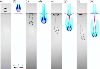
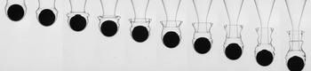
Four stages of the quasi-static detachment of a 14 mm diameter polyacetal sphere from a V500/water–glycerine interface. (a–d) Experimental sequence, the dashed line representing the corresponding static meniscus profile obtained by solving numerically the Young–Laplace problem (see appendix B; the film coating the spherical cap located below the meniscus is neglected in this approach). (e–h) Numerical sequence at the same instants of time, with levels of azimuthal vorticity $\unicode[STIX]{x1D714}_{a}=\unicode[STIX]{x2202}u_{r}/\unicode[STIX]{x2202}z-\unicode[STIX]{x2202}u_{z}/\unicode[STIX]{x2202}r$ , from $-0.1$ to $+0.1$ , according to the colour scale; the thick solid line materializing the interface is actually made of iso-contours $C=0.1$ , 0.3, 0.5, 0.7, 0.9 of the volume fraction defined in (2.1).

The static force analysis developed in § 4 of PM1 led to the conclusion that flotation of the sphere at the interface is possible only if $\unicode[STIX]{x1D701}_{p}/\unicode[STIX]{x1D701}\leqslant 3/2Bo+1/2+3/4(\log (4/Bo^{1/2})-\unicode[STIX]{x1D6FE}_{E})$ (equation (4.4) in PM1) for Bond numbers up to $\mathit{O}(1)$ , $\unicode[STIX]{x1D6FE}_{E}$ denoting the Euler constant. Therefore it can be concluded that, given its weight and the magnitude of the buoyancy and capillary forces, the sphere cannot float under the present conditions. However the ratio $\unicode[STIX]{x1D701}_{p}/\unicode[STIX]{x1D701}$ is only slightly larger than the sum of the terms in the right-hand side of the above inequality (see figure 7 of PM1), so that the sphere is expected to detach slowly from the interface. This is indeed the case, and we observed that it takes approximatively 30 s for the meniscus to pinch off and the sphere to start settling in the lower fluid.

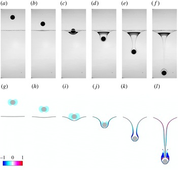
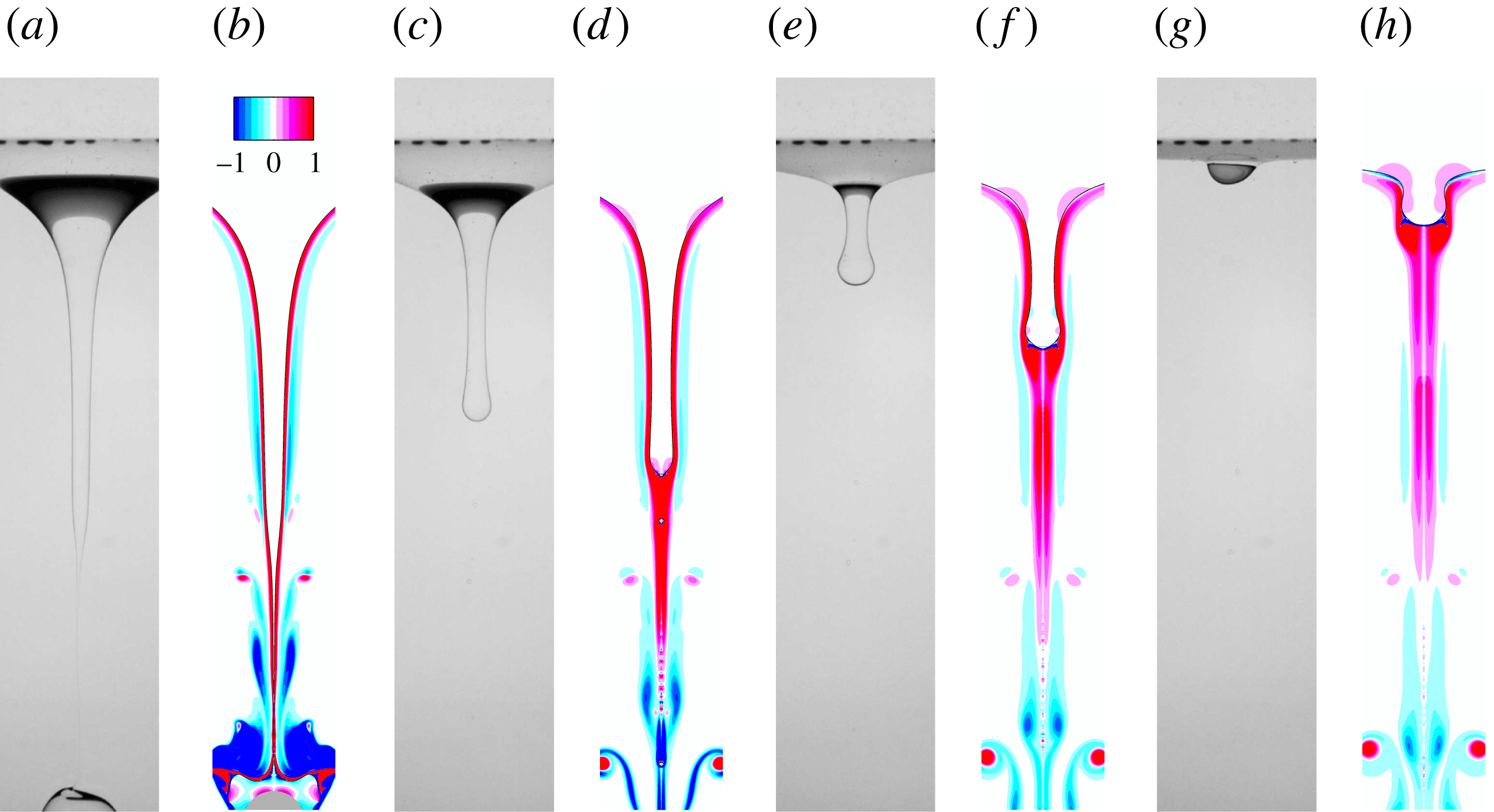
Figure 1 displays four snapshots of the meniscus evolution, from the time at which the sphere is half-immersed in each fluid to that at which it stands entirely below the initial position of the interface. These four views are selected because they correspond to specific values of the angle $\unicode[STIX]{x1D713}$ at which the film located ahead of the sphere and the meniscus match, namely $\unicode[STIX]{x1D713}=3\unicode[STIX]{x03C0}/8$ , $\unicode[STIX]{x03C0}/2$ , $5\unicode[STIX]{x03C0}/8$ and $3\unicode[STIX]{x03C0}/4$ , respectively (with $\unicode[STIX]{x1D713}=0$ at the sphere bottom). Figure 1(a–d) compares the experimental shape of the interface with the prediction provided by the numerical solution of the Young–Laplace problem (see (B 1)–(B 2) in appendix B). The agreement is very good, indicating that the system essentially undergoes a quasi-static evolution. The experimental and computational sequences show the progressive drainage of the film which first forms ahead of the sphere. As $\unicode[STIX]{x1D713}$ increases, the change in the interface curvature in the subregion where the film and the meniscus match becomes more abrupt and locally induces a large pressure gradient within the inner (i.e. upper) fluid. The corresponding fluid acceleration results in a ‘dimple’ of the film near the equator of the sphere when $\unicode[STIX]{x1D713}$ becomes close to $\unicode[STIX]{x03C0}/2$ (figure 1 b,f), in line with the asymptotic prediction of Jones & Wilson (Reference Jones and Wilson1978). Throughout the sequence, one may notice a region of positive vorticity in the lower fluid in the meniscus region; it originates in the negative radial velocities going with the deformation of the interface, first all along the meniscus (panel e), then in the dimple subregion (f,g) and eventually above the neck (h). This last frame corresponds to the stage at which the meniscus is close to snapping: as shown by O’Brien (Reference O’Brien1996), the Young–Laplace problem does not have a solution for all $\unicode[STIX]{x1D713}$ and, in the low- $Bo$ limit, a static equilibrium is not possible when $\unicode[STIX]{x1D713}\gtrsim 3\unicode[STIX]{x03C0}/4$ . Hence somewhat later the sphere starts falling freely in the lower fluid.

Figure 2.

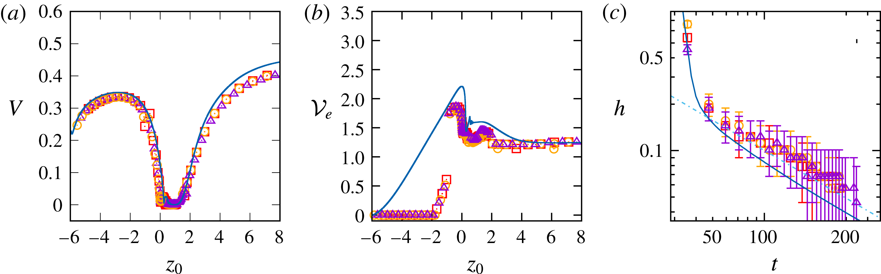
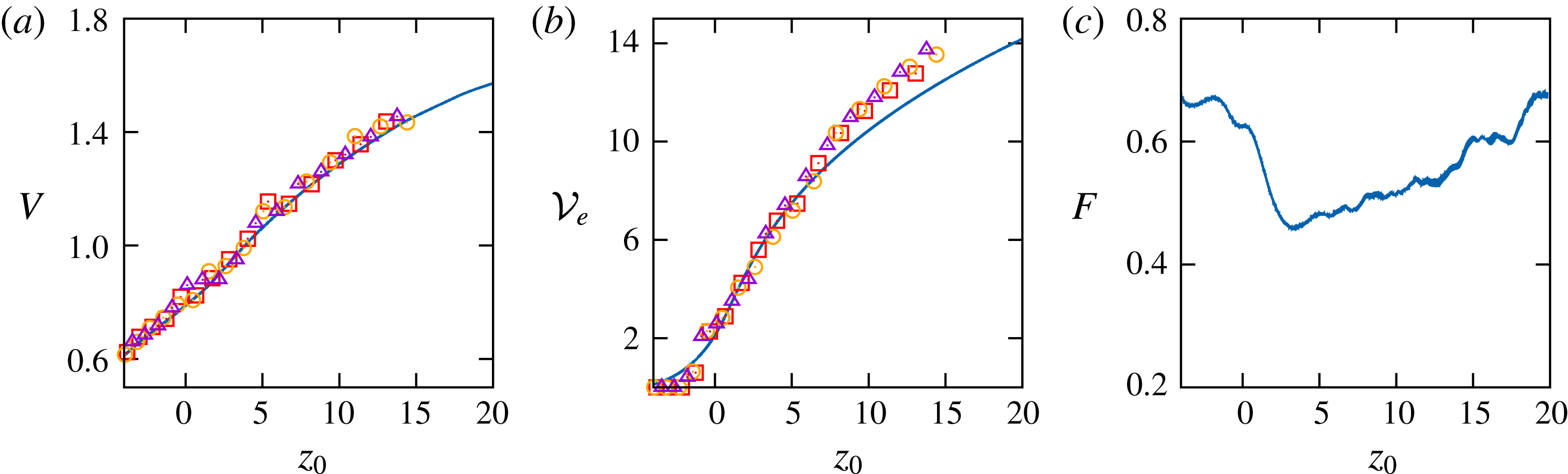
Evolution of three characteristics of the quasi-static breakthrough in the configuration considered in figure 1. (a) Settling velocity $V$ as a function of the distance $z_{0}$ from the sphere centre to the initial position of the interface; (b) displaced volume ${\mathcal{V}}_{e}$ from the initial position of the sphere ( $z_{0}\rightarrow -\infty$ ) until its current position; (c) film thickness $h(t)$ at the bottom of the sphere. Solid line: computational prediction; triangles, squares and circles refer to three different experimental tests. In (c), the dash-dotted line is a guide to the eye with a $-0.65$ slope; the experimental uncertainty $\unicode[STIX]{x0394}h$ is estimated to $\pm 3$ pixels, making $\unicode[STIX]{x0394}h/h$ increase as $h\rightarrow 0$ .

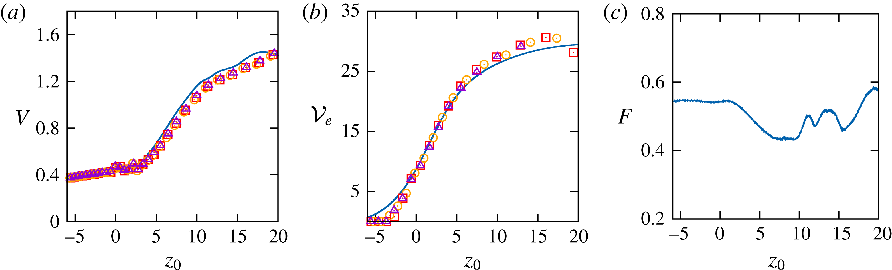
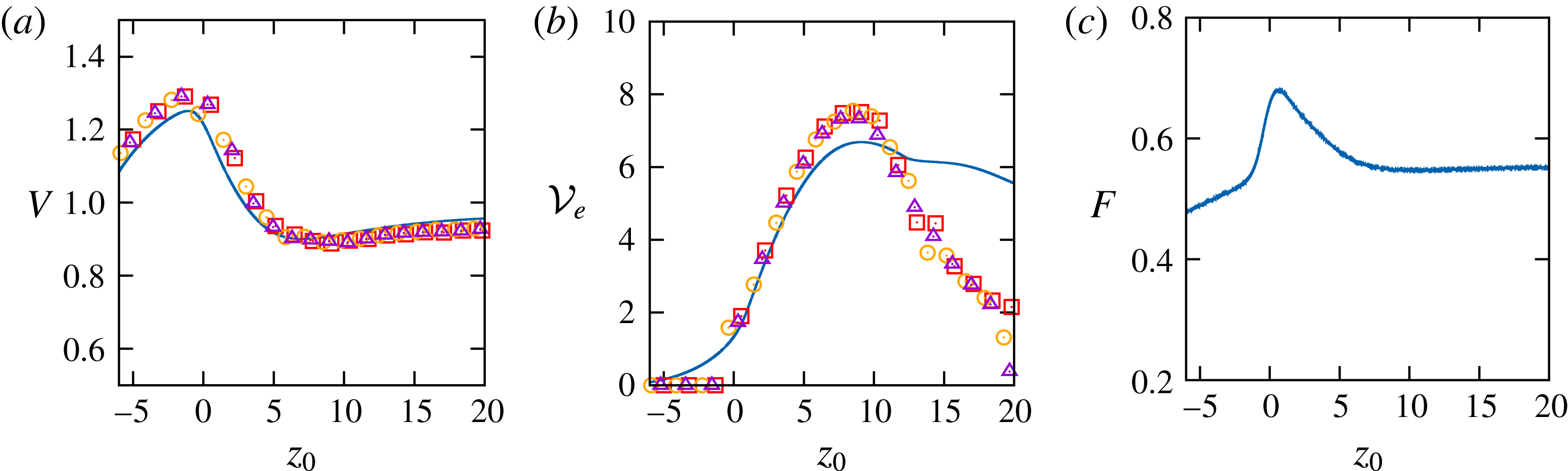
Figure 2 shows how three key characteristics of this flow configuration, namely the sphere velocity $V$ , the volume ${\mathcal{V}}_{e}$ displaced through the lower fluid and the film thickness $h$ ahead of the sphere, vary with the position $z_{0}$ of the sphere centre of mass (defined with respect to the initial position of the interface, with $z_{0}<0$ (respectively ${>}0$ ) when the sphere stands above (respectively below) the interface). As shown in figure 2(a), after having reached its equilibrium value $V\approx 0.35$ in the upper fluid, the sphere velocity starts decreasing sharply one diameter above the interface ( $z_{0}\approx -2$ ). It falls to zero and remains negligibly small within the range $0\leqslant z_{0}\leqslant 1.5$ corresponding to figure 1(a–d). The meniscus snaps when the sphere stands at $z_{0}\approx 1.5$ , as will be confirmed by examining figure 2(b). Then the sphere is released in the lower fluid and accelerates progressively. Computational and experimental evolutions are in excellent agreement up to $z_{0}=2.5$ . The 9 % overestimate of the final settling velocity is due to a slight underestimate in the film thickness and entrained drop volume, ${\mathcal{V}}_{d}$ : the net weight of the compound settling body being $(\unicode[STIX]{x1D70C}_{p}-\unicode[STIX]{x1D70C}_{2})g{\mathcal{V}}(1-\unicode[STIX]{x1D701}/(\unicode[STIX]{x1D701}_{p}-\unicode[STIX]{x1D701})({\mathcal{V}}_{d}/{\mathcal{V}}))$ , with here $\unicode[STIX]{x1D701}/(\unicode[STIX]{x1D701}_{p}-\unicode[STIX]{x1D701})\approx 1.54$ , an underestimate of the relative entrained volume ${\mathcal{V}}_{d}/{\mathcal{V}}$ by 0.035 is sufficient to generate the observed overestimate in $V$ . Assuming that the shape of the compound body is close to a sphere, this corresponds to a 1 % underestimate in its equivalent radius, which is consistent with the limitation imposed by the computational grid, which in this case involves 100 cells per sphere radius.

Figure 2(b) shows how the displaced volume ${\mathcal{V}}_{e}$ , defined as the volume comprised between the current and initial positions of the interface, i.e. ${\mathcal{V}}_{e}(t)=$ $2\unicode[STIX]{x03C0}\int _{z<0}C(r,z,t)r\,\text{d}r\,\text{d}z$ , varies with $z_{0}$ (note that this volume includes that of the sphere, so that the normalized entrained volume of light fluid ${\mathcal{V}}_{d}/{\mathcal{V}}$ equals ${\mathcal{V}}_{e}-1$ ). The computational prediction indicates that ${\mathcal{V}}_{e}$ increases almost linearly from $z_{0}\approx -6$ to $z_{0}=0$ ( $z_{0}=0$ corresponds to figure 1 a), where the displaced volume of fluid approximately equals that of the sphere. Hence the interface starts deforming well before the sphere gets close to it. This is of course the signature of the slow spatial decay of the disturbance generated by the sphere in the present $\mathit{O}(1)$ Reynolds number regime. Owing to a combination of limitations inherent to optical resolution, finite field of view and post-processing procedure, this early growth of ${\mathcal{V}}_{e}$ is not captured in experimental data, where interface deformations appear only much later, when $z_{0}\approx -2$ . However the two determinations further converge, providing similar peak values at $z_{0}=0$ and being in good agreement in later stages. Starting from its maximum at $z_{0}=0$ , ${\mathcal{V}}_{e}$ first decreases sharply due to film drainage. Then it increases again slightly owing to the lengthening of the meniscus, until the latter snaps at $z_{0}\approx 1.5$ . The upper part of the meniscus then recedes toward the initial position of the interface, making ${\mathcal{V}}_{e}-1$ decrease towards a non-zero final value of approximately 0.2 (note the good agreement between the experimental and computational final values, although the latter is slightly smaller than the former, in line with the aforementioned underestimate). The latter is provided by the lower part of the meniscus which recedes toward the sphere, giving birth to a spherical cap drop attached to its top part and approximately limited by the cap angle $\unicode[STIX]{x1D713}_{d}=3\unicode[STIX]{x03C0}/4$ at which the meniscus snapped. The way the volume of drops remaining attached to the sphere varies with the dimensionless parameters of the system was discussed in § 5 of PM1. It was shown that when the viscosity ratio is large and the sphere is light, i.e. $\unicode[STIX]{x1D706}\gg 1$ and $\unicode[STIX]{x1D701}_{p}/\unicode[STIX]{x1D701}=\mathit{O}(1)$ , the drop volume is close to that found under static conditions in the so-called pendant drop configuration. For that problem, predictions resulting from the numerical solution of the Young–Laplace problem are available in the literature (Shoukry, Hafez & Hartland Reference Shoukry, Hafez and Hartland1975; Smith & Van de Den Reference Smith and Van de Den1985). Fitting corresponding results revealed that the drop volume varies approximately as ${\mathcal{V}}_{e}-1=0.89Bo^{-1.12}$ . In the present case, $Bo=3.65$ , so that this fit indicates that ${\mathcal{V}}_{e}-1$ should be approximately 0.21, in excellent agreement with the final value observed in figure 2(b). It is interesting to notice that, in an attempt to predict the motion of small porous spheres across a sharp stratification separating two miscible fluids, Camassa et al. (Reference Camassa, Khatri, McLaughlin, Prairie, White and Yu2013) developed a model in which Stokes drag, buoyancy and the instantaneous sphere weight are in balance. They found that this model was unable to predict correctly the retention time of the sphere at the interface, unless its radius was increased so as to take into account schematically the entrainment of light fluid, thus modifying the effective buoyancy force. Yick et al. (Reference Yick, Torres, Peacock and Stocker2009) also examined the influence of fluid entrainment on the drag of a sphere settling in a linearly stratified fluid and showed that drag enhancement is essentially due to the entrainment of light fluid within a thin region surrounding the sphere, the size of which is determined by the fluid viscosity and the Brunt–Väisälä frequency. Here, the fluids are immiscible and entrainment of light fluid takes the form of an attached drop, which indeed decreases the net weight of the compound body by nearly 30 % and slightly increases the friction drag, thus significantly delaying the release of the sphere in the lower fluid.

The evolution of the dimensionless film thickness $h(t)$ at the bottom of the sphere is shown in figure 2(c). During a first stage, $h$ quickly decreases since the sphere is not yet slowed down by the interface. Then the film starts to be drained when $h\lesssim 0.2$ , which yields a $t^{-0.65}$ decrease at later times. Experimental and computational results are in fairly good agreement throughout this two-stage evolution and both of them exhibit the above decay law (differences noticed during the drainage are most likely related to the treatment of the transition region around the sphere in the IBM technique, and the aforementioned limitation of the spatial resolution). The decay observed in figure 2(c) is somewhat faster than the well-known $t^{-1/2}$ law derived by Hartland (Reference Hartland1969) and Jones & Wilson (Reference Jones and Wilson1978). The most probable reason for this difference is the influence of buoyancy, which was neglected in these two studies. Indeed, Smith & Van de Ven (Reference Smith and Van de Ven1984) showed that buoyancy effects due to the density contrast between the two fluids reduce the film thickness in the region close to the symmetry axis of the system (i.e. near the bottom of the sphere), thus accelerating the drainage. Considering the present situation with $Bo=3.7$ in which the drainage starts approximately when $h=0.2$ , their results with $\unicode[STIX]{x1D713}=\unicode[STIX]{x03C0}/3$ indicate that the time it takes for the bottom region of the film to be entirely drained (i.e. $h=0$ ) is two orders of magnitude shorter than in the low Bond number limit, giving strong credit to a faster decrease of $h(t)$ due to buoyancy in the present case.

3.2 When the sphere hesitates

We now consider the motion and flow induced by a 7 mm diameter polyacetal sphere settling through a V5/water–glycerine arrangement. This situation (which corresponds to configuration $13a$ in PM1) is quite similar to that examined above, except that the upper fluid is a hundred times less viscous and somewhat lighter. The corresponding dimensionless parameters are $Ar=86$ , $Bo=1.1$ , $\unicode[STIX]{x1D706}=18.3$ , $\unicode[STIX]{x1D701}=0.32$ and $\unicode[STIX]{x1D701}_{p}=0.48$ . 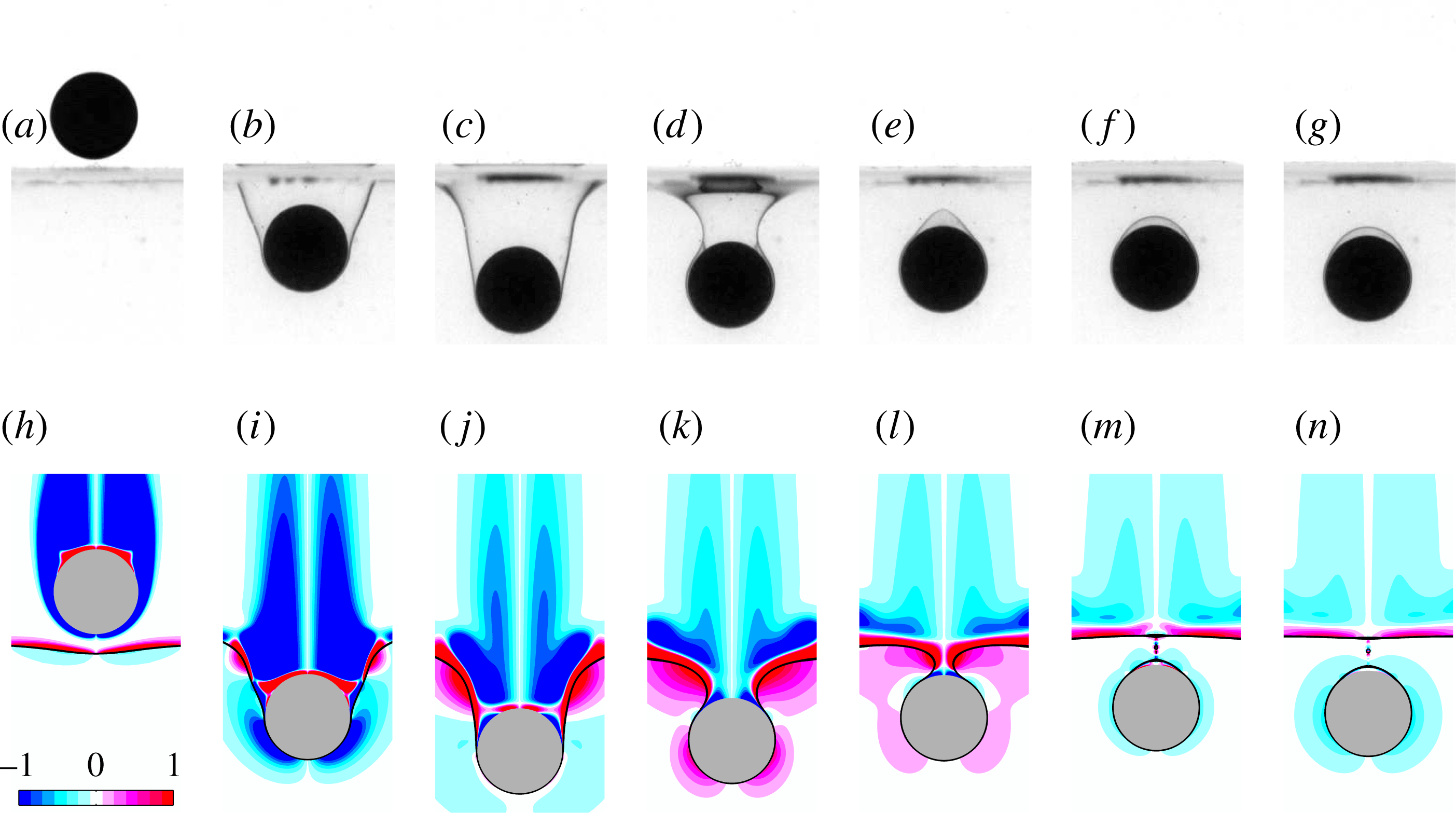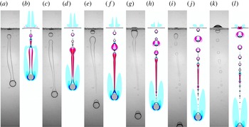According to the flotation criterion mentioned above, the sphere would float at the interface if released from rest just above it (we performed this test and found that the sphere was still floating 24 h after it was released). However, under the present conditions, it reaches the interface with a significant velocity. As figure 3 shows, it turns out that the corresponding kinetic energy is sufficient to overcome capillary effects, allowing the sphere to detach from the interface (the inertial mechanisms involved in this process were discussed in § 4 of PM1). However, owing to the strong viscosity contrast, the Archimedes number in the lower fluid is only $Ar_{l}\approx 3.2$ . Hence viscous effects are expected to play an important role in the post-detachment stage. Moreover the fluid density contrast is significant, so that the apparent weight of the sphere is reduced by one-third in the lower fluid. These two characteristics hamper its penetration in that fluid and generate a ‘rebound’ during which its velocity is positive, so that the sphere tends to come back toward the interface (figure 3 d,e,k,l). A similar reversal of the motion of a sphere sedimenting in a sharp two-layer configuration with fresh water on top of salt water was reported by Abaid et al. (Reference Abaid, Adalsteinsson, Agyapong and McLaughlin2004), who modelled the phenomenon by considering the effective buoyancy force resulting from the entrained fluid.

Figure 3.

A 7 mm diameter polyacetal sphere settling in the V5/water–glycerine pair of fluids. (a–g) Experimental sequence; (h–n) numerical sequence at the same instants of time (see figure 1 for legend); the time interval between two panels is $\unicode[STIX]{x0394}t=2.2$ .

Comparing interface shapes in figure 3(a–d) with those of figure 1 suggests that the meniscus does not obey a quasi-static equilibrium in the present case. Indeed, the maximum ‘submergence’ (i.e. the distance from the sphere centre to the initial interface) found under quasi-static conditions in the limit $Bo\ll 1$ (see equation (4.3) in PM1) is approximately 1.2 while it is twice as large in figure 3(c). This larger submergence is made possible by the collapse of the sphere wake which provides an additional downward impulse (see the evolution of the vorticity distribution in the upper fluid in figure 3 i,j). Then, when this collapse is completed, the residual kinetic energy of the sphere+fluid system is no longer sufficient to balance the large buoyancy effects resulting from the deflection of the meniscus (see § 4 in PM1), forcing the meniscus to recede in order to lower its height. This recession is accompanied by the rise of the sphere. At the same time, fluid is expelled upward from the neck of the meniscus, generating positive vorticity on both sides of the interface since the lower fluid is much more viscous and thus rises more slowly (figure 3 l). Owing to volume conservation, this upward fluid motion forces the neck to shrink, making the meniscus enter an unstable state and leading inescapably to its pinch-off. The sphere may then fall in the lower fluid with a small drop of light fluid standing on its top part and still connected to the very thin film which goes on coating the rest of its surface (figure 3 f,g,m,n).

Figure 4.

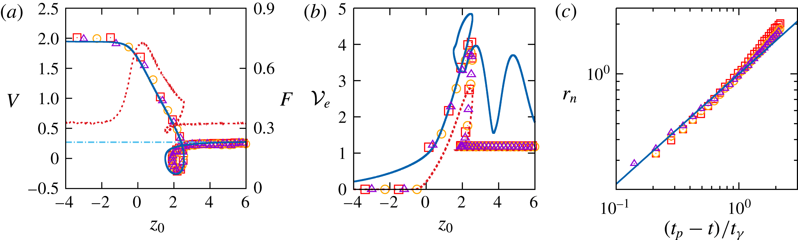
Evolution of four characteristics of the configuration considered in figure 3. (a) Settling velocity $V(z_{0})$ and effective drag force $F(z_{0})$ ; (b) displaced volume ${\mathcal{V}}_{e}(z_{0})$ ; (c) radius $r_{n}(t)$ of the neck. Triangles, squares and circles refer to three different experiments. In (a), the solid and dotted lines refer to the computational prediction for $V$ and $F$ , respectively, and the dash-dotted line corresponds to the Oseen prediction for $V$ ; in (b) the solid and dotted lines refer to the entrained volume computed as $2\unicode[STIX]{x03C0}\int _{z<0}Cr\,\text{d}r\,\text{d}z$ and $2\unicode[STIX]{x03C0}\int _{z<-1}Cr\,\text{d}r\,\text{d}z$ , respectively; in (c) the solid line is the best fit of experimental data with a $2/3$ slope and $t_{\unicode[STIX]{x1D6FE}}$ stands for the capillary time scale, $t_{\unicode[STIX]{x1D6FE}}=(\unicode[STIX]{x1D70C}R^{3}/\unicode[STIX]{x1D6FE})^{1/2}$ .

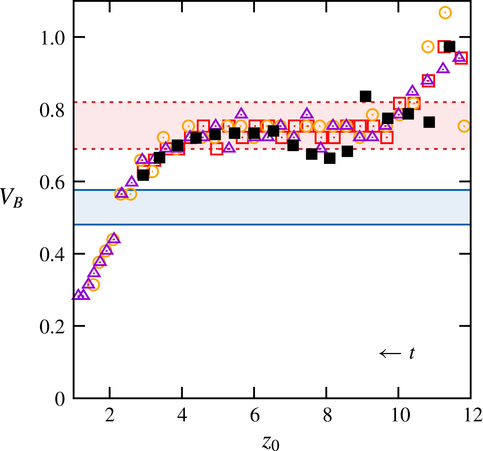
Figure 4(a) reveals that $V$ starts decreasing only when $z_{0}\approx -1$ , i.e. when the sphere almost touches the interface. Somewhat earlier, the dimensionless vertical force, $F=\boldsymbol{F}\boldsymbol{\cdot }\boldsymbol{e}_{\boldsymbol{z}}$ , defined from (2.7) as $\unicode[STIX]{x1D70C}_{p}g{\mathcal{V}}F=\boldsymbol{e}_{\boldsymbol{z}}\boldsymbol{\cdot }\int _{{\mathcal{S}}}\unicode[STIX]{x1D72E}\boldsymbol{\cdot }\boldsymbol{n}\,\text{d}S-\unicode[STIX]{x1D70C}_{1}{\mathcal{V}}g$ ( $\boldsymbol{e}_{\boldsymbol{z}}$ being the unit vector in the vertical direction), starts to increase sharply (this definition implies that $F\rightarrow \unicode[STIX]{x1D701}_{p}/(1+\unicode[STIX]{x1D701}_{p})$ when $z_{0}\rightarrow \pm \infty$ if the sphere moves with constant velocity). This is the consequence of the large viscosity of the lower fluid and of the significant fluid density contrast: both make the interface hard to deform, so that the present situation resembles that of a sphere sedimenting toward a horizontal rigid wall. The force more than doubles from $z_{0}=-2$ to $z_{0}=0$ . A splitting of this force at $z_{0}=0$ (not shown in the figure) indicates that the capillary component and the extra buoyancy components resulting from the fluid density contrast and the deflection of the meniscus (i.e. the contributions associated with volumes ${\mathcal{V}}_{cyl}$ and ${\mathcal{V}}_{spc}$ in (4.1) of PM1) contribute to $F$ by 40 % and 20 %, respectively, the last 40 % being provided by the dynamic component, essentially through the quasi-steady drag. The velocity goes on decreasing linearly almost up to the maximum submergence, $z_{0}\approx 2.5$ , where $V$ falls abruptly to zero. The force experienced by the sphere decreases regularly from $z_{0}=0$ to $z_{0}=2.5$ , where the total static contribution (not shown) made of the capillary force plus the various buoyancy contributions is found to be about $1.85F$ , owing to the large buoyancy force induced by the light fluid enclosed in the meniscus. This splitting is interesting because it reveals that dynamic effects related to the sphere deceleration provide a large negative (i.e. downward) contribution, about $-0.85F$ , so that the resulting hydrodynamic force is only $F$ . After the sphere has reached the position $z_{0}=2.5$ , the sign of its velocity reverses and it rises up to $z_{0}\approx 1.5$ , where $V$ vanishes again. This rise is associated with a decrease in $F$ , since the drag resulting from this upward motion is directed downward. It may be noticed that a loop, qualitatively similar to that observed here, was also observed in several of the aforementioned experiments by Abaid et al. (Reference Abaid, Adalsteinsson, Agyapong and McLaughlin2004). As the fluids were miscible in that case, this similarity indicates that buoyancy alone is capable of generating this intriguing behaviour. When the sphere is eventually released in the lower fluid, $V$ recovers its initial sign and quickly reaches its final value, $V_{T}$ . As $Ar_{l}$ is of $\mathit{O}(1)$ , $V_{T}$ may be compared with Oseen’s prediction. In the latter, the dimensional drag force is $6\unicode[STIX]{x03C0}\unicode[STIX]{x1D707}_{2}RV_{T}^{\ast }(1+(3/8)Re_{T})$ (Batchelor Reference Batchelor1967), with $Re_{T}=\unicode[STIX]{x1D70C}_{2}RV_{T}^{\ast }/\unicode[STIX]{x1D707}_{2}$ and $V_{T}^{\ast }=(\unicode[STIX]{x1D701}_{p}gR)^{1/2}V_{T}$ , which yields $V_{T}=(4/3)((\unicode[STIX]{x1D701}_{p}-\unicode[STIX]{x1D701})/\unicode[STIX]{x1D701}_{p}(1+\unicode[STIX]{x1D701}))^{1/2}Ar_{l}^{-1}\{-1+(1+Ar_{l}^{2}/3)^{1/2}\}$ . As shown in figure 4(a), this prediction is in excellent agreement with the experimental and computational observations.

Figure 4(b) shows that the entrained volume of light fluid is about three times that of the sphere when the meniscus reaches its maximum depth $(z_{0}\approx 2.5)$ . At later times, the entrained volume computed through the usual definition ${\mathcal{V}}_{e}=2\unicode[STIX]{x03C0}\int _{z<0}Cr\,\text{d}r\,\text{d}z$ exhibits an oscillatory behaviour, the origin of which stands in the capillary-gravity waves which develop on the interface after the meniscus has snapped. To avoid these oscillations which have nothing to do with the volume entrained by the sphere (although they are a genuine feature of the flow field), we remove the top part of the integration domain and define a modified entrained volume ${\mathcal{V}}_{em}=2\unicode[STIX]{x03C0}\int _{z<-1}Cr\,\text{d}r\,\text{d}z$ . Although it obviously underestimates the rise and maximum of ${\mathcal{V}}_{e}$ for $z_{0}\leqslant 2.5$ , the evolution of ${\mathcal{V}}_{em}$ agrees well with the experimental determination of ${\mathcal{V}}_{e}$ once the meniscus has snapped, and both indicate that the sphere eventually carries a thin drop with a volume approximately $0.15{\mathcal{V}}$ . The above agreement between the terminal velocity of the compound sphere and Oseen’s prediction indicates that the drop has little net effect on the drag, which may seem surprising since its presence increases the overall buoyancy force by nearly 30 %. The reason for this lies in the large viscosity ratio ( $\unicode[STIX]{x1D706}=18.3$ ): as shown by Johnson (Reference Johnson1981), the recirculating flow within the drop, which is significant when $\unicode[STIX]{x1D706}$ is large, decreases the net drag on the compound sphere. Here it turns out that the two effects almost compensate each other.

During the stage when the sphere rises, a ‘neck’ forms on the meniscus (see figure 3(d,k,l), where pinch-off eventually takes place. The evolution of the neck radius, $r_{n}$ , determined from experimental data, is plotted in figure 4(c) versus the time difference $(t_{p}-t)/t_{\unicode[STIX]{x1D6FE}}$ , where $t_{p}$ is the time at which pinch-off happens and $t_{\unicode[STIX]{x1D6FE}}=(\unicode[STIX]{x1D70C}R^{3}/\unicode[STIX]{x1D6FE})^{1/2}$ denotes the capillary time scale. For $(t_{p}-t)/t_{\unicode[STIX]{x1D6FE}}$ of $\mathit{O}(1)$ or less, data are found to closely follow the power law $r_{n}(t)\propto (t_{p}-t)^{2/3}$ corresponding to the self-similar behaviour of a capillary contraction in which the fluid contained within a volume of $\mathit{O}(r_{n}^{3})$ exits through a surface with an area of $\mathit{O}(r_{n}^{2})$ (Marmottant & Villermaux Reference Marmottant and Villermaux2004a ; Eggers & Villermaux Reference Eggers and Villermaux2008).

4.1 When some more inertia makes life easier

Keeping the two fluids and the sphere size unchanged with respect to the previous subsection, we first consider the flow and interface evolution generated by the settling of a glass sphere instead of a polyacetal one (configuration $14a$ in PM1). 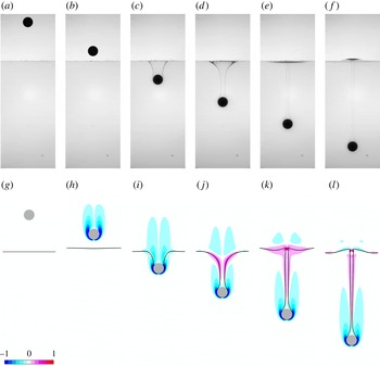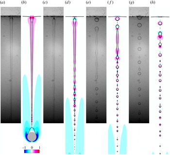Hence we still have $Bo=1.1$ , $\unicode[STIX]{x1D706}=18.3$ and $\unicode[STIX]{x1D701}=0.32$ , but now $\unicode[STIX]{x1D701}_{p}=1.74$ (instead of 0.48) and $Ar=164$ (instead of 86). As the experimental sequence in figure 5 reveals, the penetration of the sphere into the lower fluid first generates a deep, nearly cylindrical meniscus on the upper part of which a neck promptly forms (panel (c)). This meniscus still elongates, turning into a long tail which eventually pinches off at its very top under the influence of capillary effects (panel (g)), which corresponds to a ‘shallow’ pinch-off according to the terminology of Aristoff & Bush (Reference Aristoff and Bush2009). This evolution is strikingly different from the ‘rebound’ sequence observed in the previous case, underlining the influence of the sphere-to-fluid density ratio. A noticeable feature in the present experimental sequence is the non-axisymmetric geometry of the interface. This is no surprise: although the Archimedes number is fairly small in the lower fluid ( $Ar_{l}=9.3$ ), its large value in the upper fluid is well beyond the threshold $Ar_{c}=55.0$ at which the path of a freely moving sphere becomes non-vertical (Fabre et al. Reference Fabre, Tchoufag and Magnaudet2012). Therefore the sphere does not follow a strictly vertical path before it reaches the interface and its wake is not axisymmetric, yielding a non-axisymmetric tail somewhat later. Nevertheless, the departure from axisymmetry remains moderate and the corresponding evolution is still close, at least qualitatively, to the predictions provided by axisymmetric computations, as the comparison between the two sequences in figure 5 indicates.

Here it is of interest to comment on the vorticity distribution revealed by the numerical sequence of figure 5. Examining the outer fluid along the tail, especially in snapshot (h), it is clear that the flow is almost irrotational, except in the region where vorticity generated at the sphere surface is advected upwards. In particular, vorticity remains negligibly small in that fluid along the tail, as well as below the quasi-horizontal part of the interface. This contrasts with the flow within the tail, where significant levels of vorticity are observed in snapshots (d–h). As discussed in appendix B of PM1, such a vorticity distribution results from the large viscosity contrast ( $\unicode[STIX]{x1D706}=18.3$ ), which makes the flow around the tail obey virtually a shear-free condition at the interface, limiting drastically the vorticity magnitude in the outer fluid. This situation is qualitatively similar to the one observed in impact problems at an air–water interface, where $\unicode[STIX]{x1D706}\approx 55$ under standard conditions. Looking at the upper fluid just above the quasi-horizontal part of the interface in snapshots (f) and (h), one notices that the negative vorticity left in the far wake of the sphere convects outwards along the interface. Simultaneously, vorticity of opposite sign is generated at the interface, around and below the expanding vortex ring. This vortex structure is reminiscent of that observed in the case of a sphere impacting a rigid wall (Thompson, Leweke & Hourigan Reference Thompson, Leweke and Hourigan2007). The radial motion of the ‘old’ negative vorticity is induced by its image with respect to the wall and this radial motion in turn induces a positive shear responsible for the generation of the secondary vortex ring. The strong interaction between the two rings of opposite sign stops the outward motion a short distance from the axis. Here, the sphere is seriously slowed down as it penetrates in the lower fluid (its velocity is divided by a factor of two over a $8R$ distance) owing to the combined effect of the reduced buoyancy ( $\unicode[STIX]{x1D701}=0.32$ ) and much larger viscous resistance ( $\unicode[STIX]{x1D706}=18.3$ ) in the latter. Thus, although the dynamics taking place above the nearly horizontal part of the interface is less intense than if the latter were a real wall, they are similar in nature.

Figure 5.

Passage of a 7 mm diameter glass sphere through a V5/water–glycerine interface. Experimental and computational images are taken at the same instant of time in each pair of panels; the time interval between two successive pairs is $\unicode[STIX]{x0394}t=8.4$ . See figure 1 for legend.

To save space, we do not comment in detail on the variations of the sphere velocity, entrained volume and hydrodynamic force with the vertical position, as they are qualitatively similar to those displayed in figure 9(a–c) to be discussed later. The major point is that there is no severe drop of the sphere velocity during the breakthrough, in contrast to the behaviours observed in the previous section. This is a clear indication that in the present case, capillary effects and buoyancy effects related to entrainment of the upper fluid only play a secondary role compared to inertia. The sphere velocity reaches a maximum value $V\approx 2.15$ at $z_{0}=0$ , before decreasing gently toward a terminal value $V\approx 0.8$ which is reached at $z_{0}\approx 15$ . This decrease results from both the large viscosity jump ( $\unicode[STIX]{x1D706}=18.3$ ) and the drop of the buoyancy force experienced by the sphere once it is immersed in the lower fluid ( $\unicode[STIX]{x1D701}=0.32$ ).

The late evolution of the system, after the tail separates from the flat interface, is depicted in figure 6. The initial pinch-off marks the end of the period during which the tail is stretched between the sphere and the interface. Then it behaves as a pre-elongated liquid thread embedded in a more viscous fluid, a configuration known to be prone to the development of a capillary instability (Mikami, Cox & Mason Reference Mikami, Cox and Mason1975). Indeed, an interfacial instability to be described below sets in and propagates downwards, generating a series of drops of decreasing size (panels (b–d). Then a second pinch-off takes place just above the sphere and leaves a small drop attached to its top (in between panels (f) and (h) in the numerical sequence). This second pinch-off, which is due to buoyancy effects and corresponds to the ‘deep seal’ situation identified by Aristoff & Bush (Reference Aristoff and Bush2009), is the starting point of a second instability of the same type which propagates upwards and results in another series of drops of increasing size. Simultaneously, since buoyancy effects are significant, the daughter drops resulting from the first instability (especially the biggest ones) rise toward the flat interface. They do so with a nearly constant velocity, as may be observed by tracking the position of the biggest of them between panels (f) and (l) in the numerical sequence. They eventually coalesce with the upper fluid layer, generating a local bump on the otherwise flat interface (panel (k)). The two instability fronts get closer until the tail reduces to a string of drops, the size of which decreases with depth (panel (l) and beyond).

The situation just described is typical of the so-called ‘end-pinching’ instability of liquid threads (Stone et al. Reference Stone, Bentley and Leal1986; Stone & Leal Reference Stone and Leal1989). The recession of the initial thread tip first results in a bulbous, nearly spherical end, i.e. a blob. Owing to the capillary pressure jump, the intermediate region where this blob connects to the nearly cylindrical central part of the thread corresponds to a pressure minimum, since the curvature within the thread cross-sectional plane is locally negative. If the thread viscosity is small enough compared to that of the outer fluid as it is here, this longitudinal pressure gradient drives a flow from the central cylindrical part toward this connecting region, making the pressure minimum more pronounced. This in turn forces the two radii of curvature to decrease in that region, inescapably leading to pinch-off. The process can then repeat, generating a series of daughter drops which may eventually give rise to satellite droplets (some of which are visible in the numerical sequence of figure 6) and making the cylindrical part shorten progressively. The propagation of the pinch-off process (hence of the tip position of the remaining thread) was examined from a stability viewpoint by Powers et al. (Reference Powers, Zhang, Goldstein and Stone1998) who showed that the associated propagation speed, $V_{f}$ , obeys a law of the form $V_{f}=k(\unicode[STIX]{x1D706})\unicode[STIX]{x1D6FE}/\unicode[STIX]{x1D707}_{2}$ , the pre-factor $k$ being a slightly increasing function of $\unicode[STIX]{x1D706}$ .

Here the details of the process are somewhat more complicated than in the aforementioned studies, especially because there is a significant time lag between the two primary pinch-off events and the tail cross-section varies in a non-uniform manner from top to bottom, inducing dramatic variations in the size of the successive daughter drops generated during the process. These variations hamper a quantitative comparison of the drop size with theoretical predictions elaborated in idealized configurations. This is why we postpone it to the next subsection where the tail geometry is closer to that considered in theoretical analyses. Nevertheless, according to Powers et al. (Reference Powers, Zhang, Goldstein and Stone1998), the speed at which the front of the instability propagates does not depend on the local thread radius, making a comparison of the present results with their prediction for the pre-factor $k$ possible. From the successive positions of both the upper and lower tips of what remains from the tail (snapshots (d–h) and (h–l) respectively in figure 6), one finds $V_{f}\unicode[STIX]{x1D707}_{2}/\unicode[STIX]{x1D6FE}\approx 0.69$ , which is close to the value $k(\unicode[STIX]{x1D706}=18.3)\approx 0.77$ determined by Powers et al. (Reference Powers, Zhang, Goldstein and Stone1998) using boundary integral computations (see their figure 6).

Figure 6.

Late evolution of the tail in the configuration of figure 5. The time interval between two successive pairs of panels is $\unicode[STIX]{x0394}t=4.15$ .

4.2 An archetypal end-pinching configuration with $\unicode[STIX]{x1D706}=\mathit{O}(1)$

To better explore the end-pinching regime, we now consider the situation where a 10 mm diameter Teflon sphere settles through a V50/water–glycerine set-up. The corresponding dimensionless parameters are $Bo=1.9$ , $Ar=23.1$ , $\unicode[STIX]{x1D706}=1.7$ , $\unicode[STIX]{x1D701}=0.26$ and $\unicode[STIX]{x1D701}_{p}=1.25$ .

Figure 7.

Passage of a $10$  mm diameter Teflon sphere through a V50/water–glycerine interface. Experimental (a–f) and numerical (g–l) sequences; the time interval between two successive frames in each sequence is $\unicode[STIX]{x0394}t=5.0$ . See figure 1 for legend.

The two sequences displayed in figure 7 show that the sphere penetrates into the lower fluid with only a modest velocity variation, which indicates that capillary effects play little role in the breakthrough process. A slender tail then forms and goes on connecting the sphere to the flat interface, at least up to $z_{0}\approx 18$ (panels (f) and (l)). As the tail thins down, its radius is seen to exhibit a broad minimum which gets closer to the sphere (panels (d–f) and (j–l)). At the same time, the fluid contained in the upper part of the tail tends to recede toward the initial position of the interface, as the positive vorticity levels indicate (panels (j,k)). This upward motion has two important consequences. First, given the $\mathit{O}(1)$ viscosity ratio, a significant region of heavy fluid is entrained upwards (see the positive vorticity levels in panel (k)). This upwelling disturbs the initially flat interface, generating interfacial waves. These are clearly gravity-driven waves, as their wavelength is typically ten times the capillary length $l_{c}=\{\unicode[STIX]{x1D6FE}/(\unicode[STIX]{x1D70C}_{2}{-}\unicode[STIX]{x1D70C}_{1})g\}^{1/2}$ . 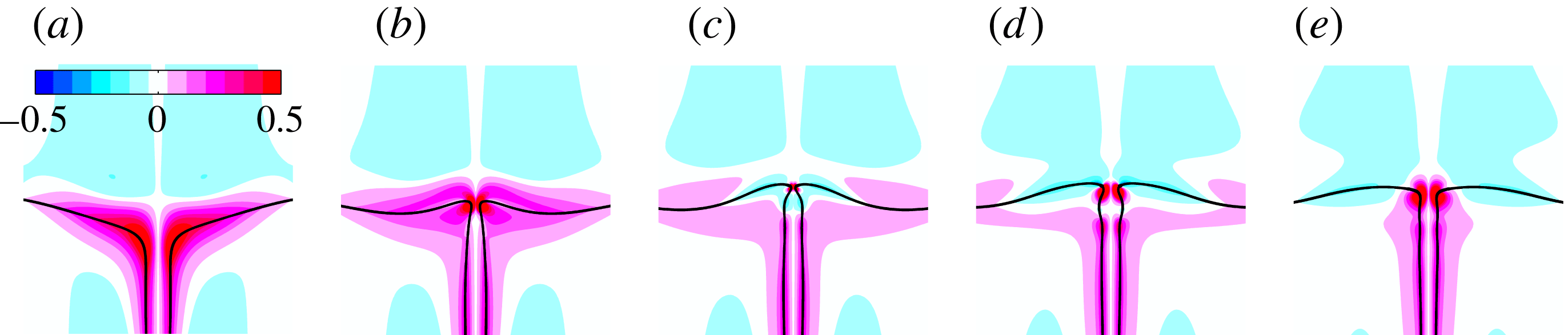Second, owing to the negative (i.e. downward) pressure gradient this flow induces along the tail, the mean curvature at the top has to decrease to satisfy the normal stress balance. As explained in the previous subsection, this yields the formation of a neck at the junction between the tail and the (almost) horizontal interface (panels (e,f) and (k,l)). Considering the situation in the last stage of figure 7, one could guess that pinch-off is going to take place at this neck. This is actually not the case, as the computational sequence displayed in figure 8 reveals. This sequence enlightens the strong coupling existing between the evolution of the neck radius and that of the vertical displacement of the wavy part of the interface: as panels (a–c) (respectively (d–f)) show, the latter experiences an upward (respectively downward) motion throughout the stage during which the neck shrinks (respectively re-opens). This one-to-one coupling may be readily understood by noting that the time rate-of-change of the interfacial energy is $(\text{d}/\text{d}t)\int _{{\mathcal{S}}_{I}}\unicode[STIX]{x1D6FE}\,\text{d}S=\unicode[STIX]{x1D6FE}\int _{{\mathcal{S}}_{I}}(\unicode[STIX]{x1D735}\boldsymbol{\cdot }\boldsymbol{n})(\boldsymbol{u}\boldsymbol{\cdot }\boldsymbol{n})\,\text{d}S$ , while that of the potential energy is $-(1/2)(\unicode[STIX]{x1D70C}_{2}{-}\unicode[STIX]{x1D70C}_{1})g(\text{d}/\text{d}t)\int _{{\mathcal{S}}_{I}}z^{2}(\boldsymbol{n}\boldsymbol{\cdot }\boldsymbol{e}_{\boldsymbol{z}})\,\text{d}S$ , where ${\mathcal{S}}_{I}$ denotes the surface separating the two fluids and $\boldsymbol{n}$ is directed towards the interior of the lower fluid. Hence, neglecting dissipative effects and variations of the kinetic energy over the whole fluid volume, when the neck narrows $(\boldsymbol{u}\boldsymbol{\cdot }\boldsymbol{n}<0)$ , the interfacial energy decreases (since the mean curvature $\unicode[STIX]{x1D735}\boldsymbol{\cdot }\boldsymbol{n}$ keeps a positive sign), and this decrease is essentially balanced by the upward displacement of the nearly horizontal part of the interface (on which the vertical component $\boldsymbol{n}\boldsymbol{\cdot }\boldsymbol{e}_{\boldsymbol{z}}$ of the normal is negative). However, the upward flow rate through the neck decreases as the neck radius goes to zero, which at some point stops the ‘feeding’ of the light fluid layer by the tail. The restoring effect of the density difference $\unicode[STIX]{x1D70C}_{2}{-}\unicode[STIX]{x1D70C}_{1}$ then drives a downward motion of the near-axis region of the wavy interface (figure 8 c–e), thus lowering the potential energy and allowing the interfacial energy to increase through a re-opening of the neck $(\boldsymbol{u}\boldsymbol{\cdot }\boldsymbol{n}>0)$ . This is how the tail escapes from pinching thanks to the restoring effect of the buoyancy force. This escape process is totally different from that identified by Hoepffner & Paré (Reference Hoepffner and Paré2013) in the case of an isolated receding liquid thread, where the key mechanism is the detachment of a vortex ring from the neck, which propagates toward the tip (i.e. through the blob) and creates a pressure loss therein.

Figure 8.

Zoom of a computational sequence showing the re-opening of the neck at the top of the tail; the time interval between two successive panels is $\unicode[STIX]{x0394}t=2.5$ .

The variations of $V$ , ${\mathcal{V}}_{e}$ and $F$ throughout the range of vertical positions of the sphere considered up to now are plotted in figure 9. Owing to the limited height of the tank, the sphere does not reach its terminal velocity before touching the interface, which is why $V$ and $F$ go on increasing until it reaches the position $z_{0}\approx -1$ (using an empirical drag law, the terminal velocity in an unbounded fluid may be approximately estimated to $1.42$ ). The mild decrease of $V$ in the range $-1\leqslant z_{0}\leqslant 8$ is mostly due to the fluid density contrast and, to a lesser extent, to the slightly larger viscosity of the lower fluid. Indeed, balancing the drag force with the net weight of the sphere and assuming the drag coefficient to be the same in both fluids, the ratio of the terminal velocities in the lower and upper fluids would be $((\unicode[STIX]{x1D701}_{p}-\unicode[STIX]{x1D701})/\unicode[STIX]{x1D701}_{p}(1+\unicode[STIX]{x1D701}))^{1/2}\approx 0.79$ , whereas if the sphere were settling in the Stokes regime, this ratio would be $(\unicode[STIX]{x1D701}_{p}-\unicode[STIX]{x1D701})/\unicode[STIX]{x1D706}\unicode[STIX]{x1D701}_{p}\approx 0.58$ . According to figure 9(a), the ratio $V(z_{0}=20)/V(z_{0}\approx 0)\approx 0.73$ lies in between these two estimates, which supports the above view. Perhaps the most interesting feature in that figure is the minimum of $V$ which may be observed at $z_{0}\approx 8$ , corresponding to the situation of figure 7(d,j). Estimates of the static forces discussed in § 4 of PM1 indicate that at this position (where the cap angle is approximately $2\unicode[STIX]{x03C0}/3$ ), the tail-induced buoyancy force is approximately 4.2 times larger than the buoyancy force acting on the sphere itself, whereas the capillary force plays virtually no role. Hence the observed minimum is a direct consequence of the maximum reached by the volume of the tail at this position. This prediction is confirmed in figure 9(b) where it is seen that the entrained volume ${\mathcal{V}}_{e}-1$ goes through a maximum value about 6.0 at $z_{0}\approx 8$ . As already observed in figure 4(b), the computational prediction greatly overestimates the tail volume at larger depths, as it becomes dominated by the contribution of the interfacial wave system which develops when $z_{0}\geqslant 11$ . Figure 9(c) shows that the force acting on the sphere experiences a significant bump when $-1\leqslant z_{0}\leqslant 8$ . A crude reasoning considering that, when the sphere crosses the position $z_{0}=0$ , half of it is immersed in each fluid and there is no meniscus (i.e. $\unicode[STIX]{x1D713}=\unicode[STIX]{x03C0}/2$ ), indicates that the corresponding contribution of the capillary force should be approximately 0.09, while that of the extra buoyancy force due to the fluid density contrast should be approximately 0.06. These estimates predict an increase of the total force about 0.15 at $z_{0}=0$ , in good agreement with the computational result.

Figure 9.

Evolution of three characteristics of the configuration considered in figure 7: (a) settling velocity $V(z_{0})$ ; (b) displaced volume ${\mathcal{V}}_{e}(z_{0})$ ; (c) effective drag force $F(z_{0})$ . For legend, see figure 4.

Figure 10.

Late evolution of the tail in the configuration of figure 7. The time step between two successive panels is $\unicode[STIX]{x0394}t=7.4$ .

Figure 10 shows how the tail evolves after its very top escaped from pinching. Whilst the sphere goes on settling, the lower part of the tail becomes very thin and pinch-off eventually takes place near the top of the sphere, which is then released in the lower fluid with an attached drop about one-third its own volume. An end-pinching sequence starts and propagates upward, generating larger drops as the front rises, owing to the increasing tail radius (panels b,d). In panel (d), satellite droplets are seen to form in between the daughter drops. Moreover, capillary waves associated with the Rayleigh–Plateau instability propagate ahead of the front. Throughout this stage, the upper half of the tail still recedes toward the horizontal part of the interface and a new neck starts to form at its very top (panels a,b). However the tail is now much thinner than it was in figure 7(j–l). Consequently the upward flow rate is much smaller and barely disturbs the horizontal interface. This is why the previously described restoring buoyancy mechanism is no longer able to stop the shrinking of the neck and a new pinch-off takes place at the top of the tail just after panels (c,d). A second end-pinching front then propagates downward. Thus the remaining slender ligament still present in panels (e,f) quickly breaks almost symmetrically from both extremities (panels g,h), generating a new series of daughter drops and satellites.

Figure 11.

Variation of the drop radius versus the local tail radius (both normalized by $R$ ). Solid line: theoretical prediction (Tomotika Reference Tomotika1935);  $\times$ , *: numerical results for the primary and satellite drops, respectively, the error bars correspond to $\pm 1$ grid cell; close (respectively open) symbols: experimental results for the primary (respectively satellite) drops, the error bars correspond to $\pm 3$ pixels.

The formation of satellite droplets is known to occur in between daughter drops, either due to the classical capillary wave instability mechanism or, as is the case here, to the end-pinching process which takes place along the cylindrical ligament left after a daughter drop has formed at each of its extremities. It has been shown to be a self-repeating process in which the larger $\unicode[STIX]{x1D706}$ the larger the number of successive generations of satellites (Tjahjadi, Stone & Ottino Reference Tjahjadi, Stone and Ottino1992). Unfortunately, neither the resolution of the camera nor that of the computational grid allows us to draw firm conclusions on this dependence from figures 6 and 10. It is much easier to compare the characteristic size of the observed daughter drops with theoretical predictions provided by linear stability theory. In the situation of interest here, namely a nearly cylindrical viscous thread surrounded by another viscous fluid at rest, the relevant theory was established in the Stokes flow limit by Tomotika (Reference Tomotika1935). Provided the density contrast between the two fluids is small and the viscosity ratio is of $\mathit{O}(1)$ , his results indicate that the wavelength of the most amplified eigenmode, $\unicode[STIX]{x1D6EC}$ , normalized by the thread radius, $R_{t}$ , depends only on $\unicode[STIX]{x1D706}$ . Specifically, for $\unicode[STIX]{x1D706}=1.7$ , his theory predicts $\unicode[STIX]{x1D6EC}/R_{t}\approx 10.65$ . Assuming that the growth of this mode eventually leads to the breakup of $\unicode[STIX]{x1D6EC}$ -long cylindrical pieces, each of which turns into a spherical drop, the radius $R_{d}$ of these drops is expected to be $R_{d}=((3/4)\unicode[STIX]{x1D6EC}R_{t}^{2})^{1/3}$ , so that $R_{d}/R_{t}\approx 2.0$ for $\unicode[STIX]{x1D706}=1.7$ . Here the tail is not cylindrical but has a slowly varying cross-section. 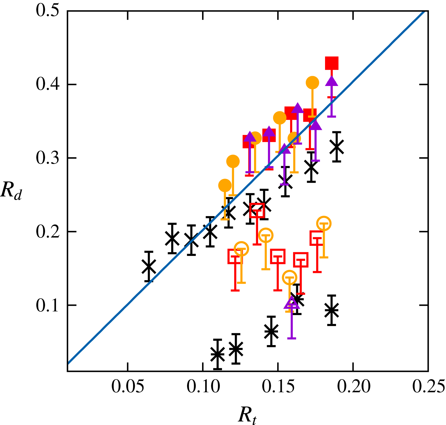Hence, in the present context, the above prediction must be considered as local, assuming that $R_{d}$ and $R_{t}$ vary slowly with the position along the tail. Considering the tail geometry just prior to the initial pinch-off in figure 10(a,b), figure 11 shows how the size of the drops identified in the experimental and computational sequences compare with Tomotika’s prediction. The lower group of data must be excluded from that comparison because it corresponds to satellite droplets, the formation of which is driven by nonlinear processes (Tjahjadi et al. Reference Tjahjadi, Stone and Ottino1992). The rest of the data display good agreement with the linear prediction, although the computational series exhibits a somewhat smaller slope, presumably because of marginally sufficient resolution. Interestingly, the inviscid linear theory (Rayleigh Reference Rayleigh1878) predicting $\unicode[STIX]{x1D6EC}/R_{t}\approx 9.02$ , i.e. $R_{d}/R_{t}\approx 1.89$ , it is observed that the stabilizing effect of viscosity increases the drop size by only 6 % in the present case.

5.1 An archetypal retraction process with $Ar_{l}=\mathit{O}(10^{3})$

We start by examining the settling of a 10 mm diameter Teflon sphere. This situation, close to that corresponding to configuration $23b$ in figure 5(b) of PM1, is characterized by dimensionless parameters $Ar=2.3$ , $Bo=0.24$ , $\unicode[STIX]{x1D706}=1.9\times 10^{-3}$ , $\unicode[STIX]{x1D701}=0.03$ and $\unicode[STIX]{x1D701}_{p}=1.23$ , hence $Ar_{l}\approx 1.19\times 10^{3}$ .

Figure 12.

Settling of a 10 mm diameter Teflon sphere through the V500/water pair of fluids. Experimental (a–f) and numerical (g–l) sequences; the time interval between two successive panels in each sequence is $\unicode[STIX]{x0394}t=4.5$ . See figure 1 for legend.

Although the Bond number is small, figure 12(b,h) indicates that the interface starts to deform well before the sphere reaches it. This is no surprise: given the modest value of $Ar$ , the spatial structure of the flow disturbance in the upper fluid is close to that corresponding to the Stokes limit, as confirmed by the approximate fore–aft symmetry of the vorticity field in figure 12(g,h). Hence the leading contribution to the velocity disturbance decays as the inverse of the distance to the sphere position (Lee, Chadwick & Leal Reference Lee, Chadwick and Leal1979), making it able to bend the interface significantly as soon as $|z_{0}|\lesssim 5$ . The Bond number being small, surface tension effects tend to maintain the deformed part of the interface broad in order to limit the increase of the interfacial energy. This contrasts with figure 7 where the Bond number is an order of magnitude larger, then allowing the development of a much more localized deflected region. The entrained column lengthens gradually and thins above the sphere. Pinch-off eventually takes place when $z_{0}\approx 20$ , leaving the top part of the sphere covered with a thick spherical cap droplet, the front part being still encapsulated in a thin film (figure 12 f,l). As may be seen in snapshots (i–k), the large viscosity contrast forces the velocity profile within any cross-section of the tail to become nearly flat, reducing gradually the magnitude of the vorticity around the sphere. In snapshot (k), the diameter of the column is still of the same order as that of the sphere, and vorticity is essentially concentrated within a thin shear layer surrounding the bottom part of the tail. It reaches its maximum just above the sphere, since the straining of the column makes the velocity of the entrained fluid maximum there. Things become different when pinch-off is about to occur (snapshot l). At that stage, the compound body made of the sphere and the drop that encapsulates it falls within the lower, low-viscosity fluid, maintaining a connection with the rest of the column only through a very thin thread. Therefore the wake which develops past the sphere is essentially similar to that past a freely translating nearly spheroidal bluff body. The corresponding Reynolds number is approximately $2.6\times 10^{3}$ , which of course promptly results in the development of a large separated wake.

Figure 13.

Evolution of three characteristics of the configuration considered in figure 12: (a) settling velocity $V(z_{0})$ ; (b) displaced volume ${\mathcal{V}}_{e}(z_{0})$ ; (c) effective drag force $F(z_{0})$ . For legend, see figure 4.

Figure 13(a) shows that the sphere velocity remains almost unaltered by interfacial effects up to $z_{0}\approx 3$ . Beyond that point, the sphere experiences a strong acceleration, tripling approximately its velocity between $z_{0}=3$ and $z_{0}=11$ . Then, the settling velocity increases more slowly, reaching its terminal value shortly after pinch-off occurs at the bottom of the tail. The ratio of the terminal velocity in the lower fluid to that in the upper one is about 3.2, close to the approximate prediction 3.4 provided by (A 3) of PM1. As shown by figure 13(b), fluid entrainment below the initial level of the interface starts significantly before the sphere has reached the corresponding position, owing to the low-Reynolds-number behaviour already pointed out. Then the entrained volume goes on increasing regularly and reaches a maximum value approximately 30 times the sphere volume. This maximum takes place before pinch-off occurs, which is not unlikely since the upper part of the column has already started to recede at that time. The force experienced by the sphere (figure 13 c) is seen to decrease sharply in the range $2\leqslant z_{0}\leqslant 7$ , owing to the small friction exerted by the low-viscosity outer fluid on the very viscous tail. This results in an increase of the sphere velocity, hence of the aforementioned friction, so that the force stops decreasing after some time and exhibits a ‘plateau’ in the range $7\leqslant z_{0}\leqslant 10$ . The development of the sphere wake for $z_{0}>10$ (i.e. in between panels (k) and (l) of figure 12) increases the energy dissipation in the outer fluid near the top of the sphere, which, on average, yields an increase of the force until it recovers a level close to its initial value. Nevertheless, oscillations due to transient effects affecting the wake, especially the release of vortex rings and the retraction of the bottom part of the column (see figure 14 below), are seen to take place during that stage.

Pinch-off takes place close to the sphere when $z_{0}\approx 22$ . As may be discerned in figure 14(a), just before it occurs, the bottom part of the very thin thread that still connects the column to the drop covering the sphere is no longer axisymmetric and exhibits some bending. Although this asymmetry is reminiscent of the coiling of viscous filaments (Ribe, Habibi & Bonn Reference Ribe, Habibi and Bonn2012), we believe that it is a manifestation of the three-dimensional effects which develop in the sphere wake, owing to the current large Reynolds number. After pinch-off happens the initially conical thread starts to recede and capillary effects quickly turn its tip into a blob (figure 14 c,d). The now nearly cylindrical thread thickens and continues to recede (figure 14 e–h) until it eventually disappears, leaving the two fluids separated by a flat interface. In contrast to the situations examined in the previous section, no end-pinching instability happens during this recession. This is in line with previous findings which showed that, in cases where $\unicode[STIX]{x1D706}\ll 1$ , the formation of a neck in the tip region is slowed down by the inner resistance of the thread, making the blob capable of receding fast enough to prevent the thread from breaking (Stone et al. Reference Stone, Bentley and Leal1986; Stone & Leal Reference Stone and Leal1989).

Figure 14.

Near- and post-pinch-off evolution of the tail; $\unicode[STIX]{x0394}t=6.0$ .

The velocity $V_{B}$ at which the tip recedes, still normalized by $(\unicode[STIX]{x1D701}_{p}gR)^{1/2}$ , is plotted as a function of its position in figure 15. After an initial deceleration (when $z_{0}\gtrsim 9$ ), experimental and numerical data exhibit a clear ‘plateau’ with $V_{B}\approx 0.75$ in the range $4\lesssim z_{0}\lesssim 9$ . In the late stage ( $z_{0}\lesssim 4$ ), the residual column thickens rapidly as it shortens, making the retraction velocity decrease sharply over time. The intermediate plateau is reminiscent of the Taylor–Culick inviscid prediction (Taylor Reference Taylor1959; Culick Reference Culick1960), according to which the capillary-driven retraction velocity of a planar sheet having a uniform thickness ${\mathcal{R}}$ is $V_{TC}=(2\unicode[STIX]{x1D6FE}/(\unicode[STIX]{x1D70C}_{1}{\mathcal{R}}))^{1/2}$ . Later, this analysis was extended to cylindrical threads by Keller (Reference Keller1983) who concluded that the same result still applies, ${\mathcal{R}}$ then being the thread radius. However, it was recently pointed out (Hoepffner & Paré Reference Hoepffner and Paré2013) that the correct velocity in that case is actually $V_{TC}=(\unicode[STIX]{x1D6FE}/(\unicode[STIX]{x1D70C}_{1}{\mathcal{R}}))^{1/2}$ . This prediction is confirmed in appendix C using a more general argument based on an exact momentum balance over the entire column, similar to that employed by Savva & Bush (Reference Savva and Bush2009) for a planar sheet. In particular, the above result is shown to hold in the presence of viscous effects, provided several conditions are satisfied. The corresponding prediction is plotted in figure 15 and is seen to underestimate the actual velocity during the plateau by more than 40 %. The analysis developed in appendix C reveals that buoyancy effects due to the density difference between the two fluids are responsible for this disagreement, their magnitude being similar to that of capillary effects. An extended version of the Taylor–Culick prediction including both effects is derived in (C 10). At short time, the modified retraction velocity is shown to be $V_{TCg}=(\unicode[STIX]{x1D701}g{\mathcal{L}}_{0}+\unicode[STIX]{x1D6FE}/(\unicode[STIX]{x1D70C}_{1}{\mathcal{R}}))^{1/2}$ , ${\mathcal{L}}_{0}$ denoting the initial length of the column. Hence the two effects cooperate in a simple manner to strengthen the retraction process, and the longer the column the larger the buoyancy contribution. As figure 15 reveals, this prediction is in excellent agreement with observations. Keeping in mind that $\unicode[STIX]{x1D701}=0.03$ in the present case, the 40 %–50 % difference between $V_{TC}$ and $V_{TCg}$ emphasizes the prominent role played by buoyancy effects, even with modest density contrasts, in the retraction dynamics.

Figure 15.

Evolution of the normalized retraction velocity $V_{B}$ of the tip of the tail as a function of its position. Dotted squares, triangles and circles refer to three different sets of experimental data, while closed squares refer to computational results. Lower horizontal band: original Taylor–Culick prediction with an average thread radius ${\mathcal{R}}_{m}$ ranging from $0.4R$ (bottom line) to $0.3R$ (top line); upper band: prediction including buoyancy effects, with the same two extreme values of ${\mathcal{R}}_{m}$ and an initial length of the column ranging from ${\mathcal{L}}_{0}=10R$ (bottom line) to ${\mathcal{L}}_{0}=15R$ (top line); see appendix C for the determination of ${\mathcal{R}}_{m}$ and ${\mathcal{L}}_{0}$ .

5.2 Increasing $Ar_{l}$ again

In this last case, we keep the same fluids arrangement as in the previous subsection but consider a bigger ( $R=7~\text{mm}$ ) and heavier (steel) sphere, which yields Bond and Archimedes numbers two and four times larger, respectively; this is the most inertial situation displayed in figure 5(b) of PM1 (configuration $27b$ ). The corresponding dimensionless parameters are now $Bo=0.46$ , $Ar=9.2$ , $\unicode[STIX]{x1D706}=1.9\times 10^{-3}$ , $\unicode[STIX]{x1D701}=0.03$ and $\unicode[STIX]{x1D701}_{p}=7.15$ , so that $Ar_{l}\approx 4.8\times 10^{3}$ .

Figure 16.

Settling of a 14 mm diameter steel sphere through the V500/water pair of fluids. Experimental (a–e) and numerical (f–j) sequences; the time interval between two successive panels in each sequence is $\unicode[STIX]{x0394}t=4.5$ . See figure 1 for legend.

In the early stages, the dynamics of the flow is very similar to that observed in the previous case. Note however that the film ahead of the sphere is drained significantly faster (compare panels (c) and (h) in figure 16 with panels (d) and (j) in figure 12). This is a direct consequence of the larger sphere inertia which yields a larger velocity at the interface of the two fluids, making the drainage easier (the thickness of the film at a given time is expected to vary as $\unicode[STIX]{x1D701}_{p}^{-1/2}$ when $\unicode[STIX]{x1D701}\approx 0$ (Hartland Reference Hartland1968, Reference Hartland1969)). The most spectacular novelty compared to the previous case occurs somewhat later, when disturbances are seen to propagate upward along the interface at the back of the sphere, generating a series of thin axisymmetric corollas or ‘inverted skirts’ around the core of the column while the latter remains attached to the sphere (panels (d,e) and (i,j)). Similar observations in the same pair of fluids were reported with large ceramic spheres by Kemiha (Reference Kemiha2006) (see Dietrich, Poncin & Li Reference Dietrich, Poncin and Li2011). The vorticity distribution around these corollas (panels (i,j)) reveals an alternation of strong positive and negative values, which is indicative of an intense generation of small-scale vortices. Visually, the phenomenon is reminiscent of the early stages of the disintegration of a cylindrical liquid jet peeled off by a fast coaxial gas stream (Marmottant & Villermaux Reference Marmottant and Villermaux2004b ). We shall see later up to which point the analogy holds.

Figure 17.

Evolution of three characteristics of the configuration considered in figure 16: (a) settling velocity $V(z_{0})$ ; (b) displaced volume ${\mathcal{V}}_{e}(z_{0})$ ; (c) effective drag force $F(z_{0})$ . For legend, see figure 4.

Figure 17(a) shows that, owing to its large inertia, the sphere accelerates throughout the whole range of positions corresponding to the viewing window (due to the limited height of the device, its velocity is only approximately 75 % of the terminal value when $z_{0}=0$ ). The settling velocity experiences a mild regular increase and displays no signature of an additional resistance when the sphere crosses the initial position of the interface, nor of a sudden increase below it, in contrast to the behaviour observed in figure 13(a). This is an indication that, throughout the sphere descent, inertia effects are large enough for the drag force to depend only weakly on the fluid viscosity. The displaced volume (figure 17 b) obeys a similar evolution. It is noticeable that its ‘final’ value at $z_{0}=20$ is about half that found in figure 13(b). Again this is an effect of the larger sphere inertia which, for a given $z_{0}$ , reduces fluid entrainment, yielding a somewhat thinner column, especially in the top region which contributes most to ${\mathcal{V}}_{e}$ (compare for instance figures 16(c) and 16(d) with figures 12(d) and 12(e), respectively). The small divergence between the experimental and numerical determinations of ${\mathcal{V}}_{e}$ observed for $z_{0}\gtrsim 7$ arises because the entire volume of fluid enclosed within the corollas artificially contributes to the entrained volume in the former, the weak optical contrast between the two fluids preventing the image processing software from discriminating them properly in that region. The mechanisms governing the evolution of the effective drag force displayed in figure 17(c) are essentially similar to those discussed in the previous subsection but two noticeable differences have to be mentioned. First, the nearly six times larger solid-to-fluid density contrast yields an approximately four times larger maximum sphere acceleration, $(\text{d}|V|/\text{d}t)_{max}\approx 0.5g$ for $z_{0}\approx 3$ , which results in a larger drop of the force. Second, the wake develops more rapidly (see figure 16 i) which corresponds to $z_{0}\approx 7$ ), making $F$ again increase as soon as $z_{0}\gtrsim 4$ , without any significant intermediate plateau.

Figure 18 displays a sequence revealing the various stages of the formation of corollas in the bottom part of the tail (the whole sequence takes place in between panels (c) and (e) of figure 16). At the very beginning, bumps are seen to form at the interface along the rear half of the sphere, quickly yielding a highly visible ring-like protrusion at its back. The top part of this protrusion then starts to hollow out and stretch in the vertical direction, giving rise to a well-defined corolla. During that time, new bumps form at the interface along the sphere, even on its front part, exhibiting crenel-like shapes with sharp angles. Once a bump has reached the top of the sphere and has transformed into a protrusion, a new corolla starts to form. Hence, after some time, the central column is surrounded by an annular region of heavy fluid which itself is surrounded by a series of thin corollas, the lowest corolla and the tail remaining connected just at the back of the sphere.

Several generic instability mechanisms may be suspected to drive the generation of this remarkable tail geometry. They may in principle be discriminated by comparing their growth rates at the most amplified wavenumber, i.e. the one corresponding to the separation distance between two successive bumps during the early stage of the instability (approximately in the second panel of figure 18). Such a comparison is attempted in appendix D. The Rayleigh–Taylor mechanism is easily ruled out because the observed wavenumber is found to lie far beyond the capillary cutoff, owing to the large capillary length. Although the strongly non-parallel geometry of the flow past the sphere may partly hamper application of classical theoretical predictions, a simple three-layer inviscid model with a piecewise linear velocity profile is then developed to examine the relevance of the Kelvin–Helmholtz mechanism. Crucial in this model is the thickness of the boundary layer in the outer fluid, which we evaluate as a function of the vertical position of the sphere by analogy with the growth of the viscous layer in Stokes’ first problem. Incorporating capillary effects into the dispersion relation, we find that the most amplified wavenumber predicted by this model closely matches visual observations. In the situation considered in § 5.1, a precursor bulge is also clearly visible on the interface near the sphere equator (panels (e,k) in figure 12) but no instability develops subsequently. In that case, the same model predicts that capillary effects are strong enough to damp the initial disturbance. These predictions give strong support to the scenario based on the Kelvin–Helmholtz mechanism. In appendix D we also examine the possibility of a viscous instability due to the large viscosity difference between the two fluids. It turns out that no theoretical result is currently available to predict the behaviour of this type of instability in the present configuration, owing to the broad range of characteristic length scales induced by the huge viscosity contrast. Nevertheless, results of two numerical investigations of the linear instability problem (Boeck & Zaleski Reference Boeck and Zaleski2005; Otto, Rossi & Boeck Reference Otto, Rossi and Boeck2013), where the behaviour of inviscid and viscous modes was compared for various fluid density contrasts, indicate that the inviscid mode dominates when $\unicode[STIX]{x1D706}\ll 1$ and $\unicode[STIX]{x1D701}\rightarrow 0$ , which corresponds to the present conditions. Hence all arguments concur to conclude that the mechanism that initiates the observed corollas is a Kelvin–Helmholtz instability.

We note that there is now a general consensus that this instability is also at the root of the primary stage of the disintegration of a liquid jet by a fast gas stream, although the role of viscous effects is still in debate (Otto et al. Reference Otto, Rossi and Boeck2013; Matas Reference Matas2015). Nevertheless, a crucial difference occurs during the next stage. In the latter case, interfacial protrusions are accelerated in the streamwise direction by the high gas velocity, resulting in a Rayleigh–Taylor instability which has been identified as responsible for the formation of longitudinal ligaments (Marmottant & Villermaux Reference Marmottant and Villermaux2004b ; Eggers & Villermaux Reference Eggers and Villermaux2008). Here, as already discussed in § 6 of PM1, the capillary length is large, making the Rayleigh–Taylor mechanism unable to amplify azimuthal disturbances within the tail. Wake instability being the only significant source left for axial symmetry breaking, corollas preserve their axisymmetry even during the late stages of their evolution, as seen in figure 16(e), until the first three-dimensional structures resulting from this instability occur in the near wake.

Figure 18.

Sequence showing the development of the corollas at the back of the sphere. The time step between two successive images is $\unicode[STIX]{x0394}t=0.6$ . Note that, although each image corresponds to a side view, the corollas are thin enough for light to cross them and reveal their inner contour, together with the shape of the central column.