1. INTRODUCTION
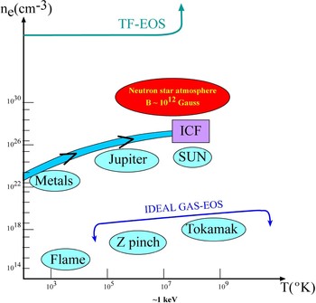
The equation of state (EOS) describes a physical system by the relation between its thermodynamic quantities, such as pressure, energy, density, entropy, specific heat, etc., and is related to both fundamental physics and the applied sciences (Lomonosov, Reference Lomonosov2007; Tahir et al., Reference Tahir, Kim, Lomonosov, Grigoriev, Piriz, Weick, Geissel and Hoffmann2007a, Reference Tahir, Kim, Matvechev, Ostrik, Lomonosov, Piriz, Lopez Cela and Hoffmann2007b, Reference Tahir, Schmidt, Brugger, Lomonosov, Shutov, Piriz, Udrea, Hoffmann and Deutsch2007c, Reference Tahir, Kim, Matveichev, Ostrik, Shutov, Lomonosov, Piriz, Lopez Cela and Hoffmann2008a, Reference Tahir, Weick, Shutov, Kim, Matveichev, Ostrik, Sultanov, Lomonosov, Piriz, Cela and Hoffmann2008b; Lebo et al., Reference Lebo, Lebo, Batani, Dezulian, Benocci, Jafer and Krousky2008). Local thermodynamic equilibrium of nature can be described by a wide range of EOS pressure, density, and temperatures. For example, Figure 1 represents schematically various systems in the temperature-electron density domain. A route to inertial confinement fusion (ICF) leading to a solution of the energy problem is shown in this figure. As can be seen from this schematic figure, the well known low density ideal EOS gas as well as the extremely high density Thomas Fermi (TF) EOS cannot describe correctly the ICF problem, and therefore more complicated (i.e., realistic) EOS are needed. Since it is not yet known how to describe quantitatively the material at every available thermodynamic state, including all phases of the matter, it is necessary to introduce simplified methods whose range of applicability is limited. So far this is the attitude taken for EOS-ICF calculations (Eliezer et al., Reference Eliezer, Murakami and Martinez-Val2007).
(Color online) The route to inertial confinement fusion (ICF) in the electron density (n) –temperature (T) plane. The Z pinch and Tokamak plasmas are described by the ideal gas equation of state (EOS), the Thomas Fermi (TF) EOS describe matter at very high densities while the route to ICF is described by complicated EOS.

The EOS is derived from a thermodynamic potential. There are equivalent thermodynamic potentials related to each other by a Legendre transformation. The Legendre transformation between two potentials F and Ψ for several variables is defined by
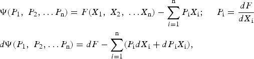
where the conjugate variable of X i is P i. For example, the conjugate variables of entropy and specific volume (S, V) are the temperature and pressure (T, P) accordingly. Assuming a system with a constant number of particles, N = const., the Gibbs potential G is derived from the internal energy E by the following Legendre transformation

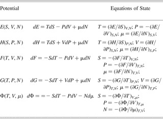
A summary of the thermodynamic potentials, derived from each other by a Legendre transformation is given in Table 1. The thermodynamic potentials are: E = internal energy, H = enthalpy, F = Helmholtz' free energy, G = Gibbs' free energy, and Φ = the grand potential. The appropriate variables of the potentials are denoted by V = specific volume = 1/ρ where ρ is the density, T = temperature, P = pressure, S = entropy, µ = chemical potential, and N = the number of particles. The various EOS derived from these potentials are summarized in Table 1. As one can see from this table, there are many possible presentations of EOS.
Equations of state for the various potentials: Specific energy E, Enthalpy H, Helmholtz Free Energy F, Gibbs potential G and the grand potential Φ. The thermodynamic variables for the potentials are given in the brackets of the first column, where the notation is: entropy – S, specific volume – V, pressure – P, temperature – T, μ is the chemical potential and the particle number is N

The starting points in analyzing the one-dimensional fluid equations described by the conservation laws of mass, momentum, and energy is given by,
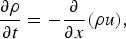


The usual notation is used, where x-t is space-time, ρ is the density, u is the flow velocity, P is the pressure, and E is the internal energy per unit mass. These three equations have four unknowns: ρ-P-E-u and therefore another equation, namely the EOS is needed in order to solve the problem.
2. SHOCK WAVES
The science of EOS (Eliezer et al., Reference Eliezer, Ghatak and Hora1986; Eliezer & Ricci, Reference Eliezer and Ricci1991; Bushman et al., Reference Bushman, Kanel, Ni and Fortov1993; Batani et al., Reference Batani, Keonig, Benuzzi, Krasyuk, Pashinin, Semenov, Lomonosov and Fortov1999, Reference Batani, Dezulian, Redaelli, Benocci, Stabile, Canova, Desai, Lucchini, Krousky, Masek, Pfeifer, Skala, Dudzak, Rus, Ullschmied, Malka, Faure, Koenig, Limpouch, Nazarov, Pepler, Nagai, Norimatsu and Nishimura2007; Desai et al., Reference Desai, Dezulian and Batani2007; Lomonosov, Reference Lomonosov2007; Eliezer & Henis, Reference Eliezer, Henis, Eliezer and Mima2008) is studied experimentally in the laboratory by using static and dynamic techniques. In static experiments, the sample is squeezed between pistons or anvils. The conditions in these static experiments are limited by the strength of the construction materials. In the dynamic experiments, shock waves are created (Zeldovich & Raizer, Reference Zeldovich and Raizer1966). Since the passage time of the shock is short in comparison with the disassembly time of the shocked sample, one can do shock wave research for any pressure that can be supplied by a driver, assuming that a proper diagnostic is available. In the scientific literature, the following shock-wave generators are discussed: a variety of guns (such as rail guns and two stage light-gas gun) that accelerate a foil to collide with a target, exploding foils, magnetic compression, chemical explosives, nuclear explosions, and high power lasers (Eliezer, Reference Eliezer2002; Evans et al., Reference Evans, Freeman, Graham, Horsfield, Rothman, Thomas and Tyrrell1996; Batani et al., Reference Batani, Bossi, Benuzzi, Koenig, Faral, Boudenne, Grandjouan, Atzeni and Temporal1996; Rothman et al., Reference Rothman, Evans, Horsfield, Graham and Thomas2002; Koening et al., 2004). Conventional high explosives and gun drivers can achieve pressures up to a few mega-bars, while with the high power lasers; up to one giga-bar pressure has been achieved. The Nova laser from Livermore laboratories created a pressure of 750 ± 200 Mbar (Cauble et al., Reference Cauble, Phillion, Hoover, Holmes, Kilkenny and Lee1993). This was achieved in a collision between two gold foils, where the flyer (Au foil) was accelerated by a high intensity X-ray flux created by the laser plasma interaction.
If the initial flow velocity is u0 ≠ 0, then the conservation laws (mass, momentum, and energy) in the laboratory frame of reference can be written
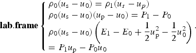
These equations are called the Hugoniot relations. These relations are used to determine the state of the compressed solid behind the shock front. Assuming that the initial state is well defined and the quantities E 0, u 0, P 0, and ρ0 are known, one has FIVE unknowns E 1, u p, P 1, ρ1, and u s with three equations. Usually the shock wave velocity is measured experimentally, and if the EOS is known (in this case, one has four equations) E = E(P, ρ) then the quantities of the compressed state can be calculated. If the EOS is not known, then one has to measure experimentally two quantities of the shocked material, for example, u s and u p, in order to solve the problem.
It was found experimentally (McQueen, Reference McQueen, Eliezer and Ricci1991) that for many solid materials, initially at rest (u 0 = 0), the following linear relation between the shock velocity u s and the particle velocity u p is valid to a very good approximation

where c 0 and α are constants. c 0 is the bulk sound speed at standard conditions, where c 0 is related to the longitudinal (c L), and transversal (c t) velocities of the sound,
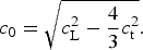
Eq. (6) is an EOS along the Hugoniot line by taking into account the Hugoniot relations, where the shock and particle velocities are expressed by the appropriate density and pressure.
The laser driven matter under extreme conditions for EOS studies is achieved by: (1) laser produced shock waves in direct drive, (2) X-ray produced shock waves in hohlraum drive, and (3) shock wave by impact with laser (direct or indirect) launched flyer plate. For accurate EOS measurements, a uniform shock wave is required, steady state pressure, and no preheating. For example, 1% accuracy in velocity measurements for ~1 mm target size and ~1 ns measurement time, it is necessary to have 10 µm spatial resolutions and 10 ps temporal resolutions.
3. IMPACT BY AN ACCELERATING FOIL
The highest laser induced pressures, ~108–109 atmospheres have been obtained during the collision of a target with an accelerating foil. This acceleration was achieved by laser-produced plasma, or by X-rays from a cavity produced by laser plasma interactions. It is therefore now shown how the pressure is calculated in a planar collision between a flyer and a target.
The flyer has a known (i.e., measured experimentally) initial velocity before impact, u f. The initial state before collision is for the target (B) u p = 0 and P = 0, while for the flyer (A) u p = uf, and P = 0. Upon impact, a shock wave moves forward into B, and another shock wave goes into the flyer in the opposite direction. The pressure and the particle velocity are continuous at the interface of target and flyer. Therefore, the particle velocity of the target changes from zero to u, while the particle velocity in the flyer changes from u f to u. Moreover, the pressure in the flyer plate A equals the pressure in the target plate B, and if the EOS are known and given by the linear u s − up relation and the second Hugoniot equation is used to calculate the pressure, one gets

This is a quadratic equation in u, with the following solution
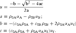
Once the flow velocity u is known, it is substituted in the above equation to derive the pressure. If the EOS of the target is not known, then it is necessary to measure the shock wave velocity u sB. In this case, the pressure equality in the flyer and the target yields

Note that in this equation, u sB is known. The solution of this equation is

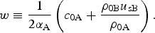
In these types of experiments, it is occasionally convenient to measure the free surface velocity of the target in order to calculate the particle velocity.
Foils are used to impact stationary targets and reach pressures of hundreds of Mega-bar. In this method, the flyer stores kinetic energy from the driver, which may be a laser or X-rays, and delivers it much rapidly as thermal energy during collisions. In addition, the flyer serves as a preheat shield so that the target remains on a lower adiabat. The flyer technique was demonstrated using a laser as driver (Obenschain et al., Reference Obenschain, Whitlock, Lean and Ripin1983) and later applied to achieve pressures of more than 100 Mbar (Fabbro et al., Reference Fabbro, Faral, Virmont, Pepin, Cottet and Romain1986). At ILE, Osaka University in Japan (H. Azechi, 2008, private communication), the highest pressure was achieved, 410 ± 60 Mbar, with a direct drive laser induced flyer. The flyer, a plastic foil of 14 µm thickness doped with 0.3% CHBr (for Rayleigh Taylor stability), was accelerated to a final velocity of 640 km/s, and during its collision with a copper target, the pressure of ~400 Mbar was achieved. At Livermore, the flyer technique was used (plastic-gold flyer on a gold target) with X-ray created by Nova to produce over ~700 Mbar in a planar shock (Cauble et al., Reference Cauble, Phillion, Hoover, Holmes, Kilkenny and Lee1993), enabling first experimental measurements of EOS in the giga-bar regime.
4. THE ELLIPSOMETRY PROPOSAL FOR LASER-PLASMA INTERACTIONS
Ellipsometry measures the polarization-dependent reflectivity of a probe beam from a surface and can distinguish the real and imaginary parts of the time dependent complex index of refraction N(ω) = n + ik, giving access to fundamental properties of the material, such as phase transitions (Nissim et al., Reference Nissim, Eliezer, Bakshi, Perelmutter, Moreno, Kot, Rozenberg and Pasternak2007) and electrical conductivity. ω is the probe laser frequency.
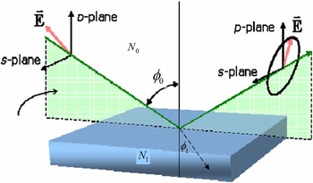
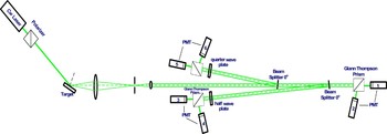
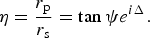
The polarization state of the light, incident upon the sample, may be decomposed into an S and a P component (the S component is oscillating perpendicular to the plane of incidence and parallel to the sample surface, and the P component is oscillating parallel to the plane of incidence, see Fig. 2). The amplitudes of the S and P components, after reflection and normalized to their initial value, are denoted by r s and r p, respectively. Ellipsometry measures the ratio η of r s and r p. The absolute value of the reflected amplitudes ratio (denoted by tan ψ) and the phase difference Δ are determined by six photo-multiplier detectors as described in Figure 3 for the general case where polarization is not necessarily 100%. Previously, Yoneda et al. (Reference Yoneda, Morikami, Ueda and More2003) suggested a scheme with four photo-multipliers where one requires 100% polarization. In our impact experiments with gas gun or even in high pressure static experiments, it was found that polarization can be reduced occasionally to 10%.
(Color online) The ellipsometry scheme. N 0 and N 1 are the complex indices of refraction, φ0 and φ1 are the incident and the reflected angle, E is the laser electric field, and s and p are the two distinct polarizations.

(Color online) The experimental set up for the ellipsometry measurements. PMT from 1 to 6 are photo multipliers. The incident diagnostic laser passes through a polarizer before hitting the target under consideration. The scattered laser is deflected by a beam splitter via a quarter wave plate to derive circular polarizations (left and right) into PMT 5 and 6. The laser that passes the first beam splitter is deflected by a second beam splitter via a half wave plate to obtain linear polarizations (at +45 and −45 degrees) into PMT 3 and 4. Finally, the PMT 1 and 2 measure the s and p polarizations. From the six PMT measurements the Stokes vector (four parameters) are calculated.

In Figure 3, the experimental setup for the ellipsometry measurement is described with six photo-multipliers (PMT). The incident diagnostic laser passes through a polarizer with an intensity I tot before hitting the target under consideration. The scattered laser is deflected by a beam splitter via a quarter wave plate to derive circular polarizations, right and left with intensities I rcp and I lcp accordingly, into PMT 5 and 6 that measure intensities I 5 and I 6. The laser that passes the first beam splitter is deflected by a second beam splitter via a half wave plate to obtain linear polarizations at +45 and −45 degrees with intensities I +45 and I −45 accordingly into PMT 3 and 4 that measure intensities I 3 and I 4. Finally, the PMT 1 and 2 measure I 1 and I 2 that corresponds to the S and P polarizations with intensities I s and I p accordingly. From the six PMT measurements, the Stokes vectors time dependent (s 0, s 1, s 2, s 3) are calculated according to the following relations

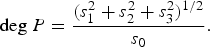
From the Stokes vector, the ratio η of the P to S polarization amplitudes is calculated for +45 degrees linear polarization laser probe beam (incident on target). Assuming that the refraction index N 0 is known, the degree of polarization, deg P, the complex index of refraction, N 1, and emissivity, ε, of the target (see Fig. 2) are derived.


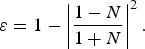
In laser induced shock waves studies, the ellipsometry is combined with other diagnostics, such as that using the velocity interferometer system for any reflector (VISAR), pyrometry or X-ray diffraction, providing a precise characterization of the dynamic properties of the material.
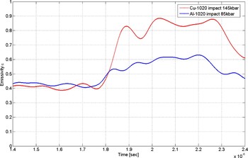
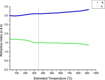
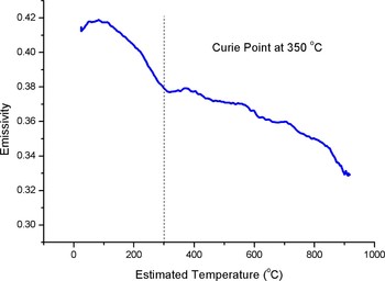
In order to show the power of ellipsometry in detecting phase transitions of the first kind (solid-solid and solid-liquid) and phase transitions of the second kind (the Curie transition), we present three very recent experiments using a 532 nm probe laser. The pressures where obtained with gas gun impact (Fig. 4), and temperatures experiments with pulsed power heating (Figs 5 and 6). In Figure 4, the emissivity change is shown during a solid-solid (α → ɛ) phase transition of 1020 steel (the upper line after the shock wave transition at 1.8 µs) in comparison with the change without a phase transition (the lower line). In Figure 5, the refractive index of nickel as a function of temperature is given where the upper line is imaginary part and the lower line the real index of refraction. Figure 6 describes the emissivity change of nickel during a phase transition of the second kind where a distinct change in the slope occurs near the Curie point. It is important to emphasize that in these experiments, all Stokes components were measured as described in Figure 3 and the above formulas.
(Color online) The emissivity change during a solid-solid (α → ɛ) phase transition of 1020 steel (the upper line after the shock wave transition at 1.8 µs) in comparison with the change without a phase transition (the lower line).

(Color online) The complex refractive index of nickel as a function of temperature. The upper line is the complex index of refraction while the lower line is the real index of refraction.

(Color online) The emissivity change of nickel during a phase transition of second kind. The Curie point there is a distinct change in the slope.

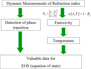
We conclude this paper with the summary given in Figure 7, where the schematic flow chart shows the connection between the complex index of refraction and the EOS. The emissivity is required in order to obtain the temperature, one of the most important thermodynamic quantities describing the EOS. The detection of the phase transition domains is an integral part of EOS.
(Color online) A schematic flow chart that shows the connection between the complex index of refraction and the equations of state.