2. Relation for invariants of FVGTs in homogeneous turbulence

We start with the relation for the invariants of the velocity gradient tensor ${\mathsf{A}}_{ij} \equiv {\partial u_i}/{\partial x_j}$, where $\boldsymbol {u}(\boldsymbol {x},t)$ is the velocity field. We use the symbol $\bar {y}^\ell$ to denote the low-pass filtering operation to any field $y(\boldsymbol x)$:

(2.1)\begin{equation} \bar{y}^\ell(\boldsymbol x) = \int_V \mathscr{G}^\ell (\boldsymbol{r})y(\boldsymbol{x} + \boldsymbol{r})\, {\rm d} \boldsymbol{r},\end{equation}

where $\mathscr {G}^\ell (\boldsymbol r)$ is the filter defined on the domain $V$. In this work, we choose the widely used Gaussian filter with $V = \mathbb {R}^3$:

(2.2)\begin{equation} \mathscr{G}^\ell(\boldsymbol{r}) = \frac{1}{(2{\rm \pi} \ell^2)^{3/2}}\, {\rm e}^{-|\boldsymbol{r}|^2/2\ell^2} , \end{equation}

which, when applied to a field, would retain spatial variations with scale larger than $\sim \ell$ but suppress those with scale smaller than $\sim \ell$. Thus $\bar {u}^\ell _i$ and $\bar {A}^\ell _{ij} \equiv {\partial \bar {u}^\ell _i}/{\partial x_j}$ refer respectively to the velocity and FVGT filtered by a Gaussian filter with size $\ell$. We restrict our discussion to incompressible flows; thus $A_{ii} = \bar {A}^\ell _{ii} = 0$. Note that a second-rank tensor can always be decomposed into its symmetric and antisymmetric parts: ${\mathsf{A}}_{ij} = {\mathsf{S}}_{ij} + {\boldsymbol{\mathsf{\Omega}}} _{ij}$, where ${\mathsf{S}}_{ij} \equiv ({\mathsf{A}}_{ij} + {A}_{ji})/2$ and ${\boldsymbol{\mathsf{\Omega}}} _{ij} \equiv ({\mathsf{A}}_{ij} - {A}_{ji})/2$. Similarly we define $\bar {S}^\ell _{ij}$ and $\bar {\varOmega }^\ell _{ij}$, with $\bar {A}^\ell _{ij} = \bar {S}^\ell _{ij} + \bar {\varOmega }^\ell _{ij}$.

Betchov (Reference Betchov1956) proved two relations for the invariants of ${\mathsf{A}}_{ij}$ in homogeneous and incompressible flows:

(2.3)\begin{equation} \langle {\mathsf{A}}_{ij} {A}_{ji} \rangle = \langle {\mathsf{A}}_{ij} A_{jk} A_{ki} \rangle = 0, \end{equation}

where the brackets $\langle \ \rangle$ denote the ensemble average. Equation (2.3) can be expressed in terms of ${\mathsf{S}}_{ij}$ and ${\boldsymbol{\mathsf{\Omega}}} _{ij}$:

(2.4)$$\begin{gather} \langle {\mathsf{S}}_{ij} S_{ji} \rangle ={-} \langle {\boldsymbol{\mathsf{\Omega}}} _{ij} \varOmega_{ji} \rangle = \tfrac{1}{2}\langle \omega_i \omega_i \rangle, \end{gather}$$

(2.5)$$\begin{gather}\langle {\mathsf{S}}_{ij} S_{jk} S_{ki} \rangle ={-} 3 \langle {\boldsymbol{\mathsf{\Omega}}} _{ij} S_{jk} \varOmega_{ki} \rangle ={-}\tfrac{3}{4} \langle \omega_i {\mathsf{S}}_{ij} \omega_j \rangle, \end{gather}$$

where $\omega _i = - \epsilon _{ijk} \varOmega _{jk}$ is the vorticity vector and $\epsilon _{ijk}$ is the permutation tensor. Equation (2.4) connects the amplitudes of vorticity and the rate of strain, while (2.5), remarkably, relates the mean rate of VS $\langle \omega _i {\mathsf{S}}_{ij} \omega _j \rangle$ to the third-order moments of strain $\langle {\mathsf{S}}_{ij} S_{jk} S_{ki}\rangle$, which provides further insight into the statistics of ${\mathsf{A}}_{ij}$ (Meneveau Reference Meneveau2011). On the other hand, using FVGT allows us to investigate the interactions between strain and vorticity with different filtered sizes (Leung et al. Reference Leung, Swaminathan and DaVidson2012; Fiscaletti et al. Reference Fiscaletti, Elsinga, Attili, Bisetti and Buxton2016b; Lozano-Durán, Holzner & Jiménez Reference Lozano-Durán, Holzner and Jiménez2016), for which (2.3) needs to be extended. To that end, we note that recently Yang et al. (Reference Yang, Fang, Fang, Pumir and Xu2022) derived a general relation for the invariants involving three vector gradient fields ${\partial a_i}/{\partial x_j}$, ${\partial b_i}/{\partial x_j}$ and ${\partial c_i}/{\partial x_j}$ in homogeneous flows:

(2.6)\begin{align} &\left \langle \frac{\partial a_i}{\partial x_j} \frac{\partial b_j}{\partial x_k} \frac{\partial c_k}{\partial x_i} \right \rangle + \left \langle \frac{\partial a_i}{\partial x_j} \frac{\partial c_j}{\partial x_k} \frac{\partial b_k}{\partial x_i} \right \rangle = \left \langle \frac{\partial a_i}{\partial x_j} \frac{\partial b_j}{\partial x_i} \frac{\partial c_k}{\partial x_k} \right \rangle + \left \langle \frac{\partial b_i}{\partial x_j} \frac{\partial c_j}{\partial x_i} \frac{\partial a_k}{\partial x_k} \right \rangle \nonumber\\ &\quad + \left \langle \frac{\partial c_i}{\partial x_j} \frac{\partial a_j}{\partial x_i} \frac{\partial b_k}{\partial x_k} \right \rangle - \left \langle \frac{\partial a_i}{\partial x_i} \frac{\partial b_j}{\partial x_j} \frac{\partial c_k}{\partial x_k} \right \rangle. \end{align}

Note that the derivation of the above only used the chain rule of derivatives and homogeneity. Special cases of (2.6) were known before. For example, Appendix D of Eyink (Reference Eyink2006) discussed the case when $a_i$, $b_i$ and $c_i$ are all solenoidal, and Yang, Pumir & Xu (Reference Yang, Pumir and Xu2020) derived the form for $a_i = b_i = c_i$ but without requiring zero divergence. Now if we choose the fields $a_i$ and $b_i$ to be the filtered velocity with filter size $\ell _1$ and $c_i$ to be the filtered velocity with a different filter size $\ell _2$, i.e. $a_i = b_i = \bar {u}^{\ell _1}_i$ and $c_i = \bar {u}^{\ell _2}_i$, (2.6) gives

(2.7)\begin{equation} \langle \bar{A}^{\ell_1}_{ik} \bar{A}^{\ell_1}_{kj} \bar{A}^{\ell_2}_{ji} \rangle = 0,\end{equation}

which can be further expressed as

(2.8) \begin{align} \langle \bar{A}^{\ell_1}_{ik} \bar{A}^{\ell_1}_{kj} \bar{A}^{\ell_2}_{ji} \rangle &= \langle (\bar{S}^{\ell_1}_{ik} + \bar{\varOmega}^{\ell_1}_{ik} ) ( \bar{S}^{\ell_1}_{kj} + \bar{\varOmega}^{\ell_1}_{kj} ) (\bar{S}^{\ell_2}_{ji} + \bar{\varOmega}^{\ell_2}_{ji} ) \rangle \nonumber\\ &= \langle \bar{S}^{\ell_1}_{ik} \bar{S}^{\ell_1}_{kj} \bar{S}^{\ell_2}_{ji} \rangle + \langle \bar{\varOmega}^{\ell_1}_{ik} \bar{\varOmega}^{\ell_1}_{kj} \bar{S}^{\ell_2}_{ji} \rangle + 2 \langle \bar{\varOmega}^{\ell_1}_{ik} \bar{S}^{\ell_1}_{kj} \bar{\varOmega}^{\ell_2}_{ji} \rangle = 0. \end{align}

Physically, we can regard $\langle \bar {S}^{\ell _1}_{ik} \bar {S}^{\ell _1}_{kj} \bar {S}^{\ell _2}_{ji} \rangle$ as the interaction between strain at scale $\ell _1$ and strain at scale $\ell _2$, $\langle \bar {\varOmega }^{\ell _1}_{ik} \bar {\varOmega }^{\ell _1}_{kj} \bar {S}^{\ell _2}_{ji} \rangle$ as the vorticity at scale $\ell _1$ stretched by the strain at scale $\ell _2$ and $\langle \bar {\varOmega }^{\ell _1}_{ik} \bar {S}^{\ell _1}_{kj} \bar {\varOmega }^{\ell _2}_{ji} \rangle$ as the interaction between strain and vorticity at scale $\ell _1$ with vorticity at scale $\ell _2$. In the next section we show that those terms in (2.8) are closely related to the SSA and VS mechanisms defined in Johnson (Reference Johnson2020), and based on (2.8) one can show that SSA contributes more to inter-scale energy transfer than VS.

3. The SSA is larger than VS

By filtering the Navier–Stokes equation, one can readily obtain the evolution equation for the filtered velocity $\bar {u}^\ell _i$:

(3.1)\begin{equation} \frac{\partial \bar{u}^\ell_i}{\partial t} + \bar{u}^\ell_j \frac{\partial \bar{u}^\ell_i}{\partial x_j} ={-}\frac{\partial \bar{p}^\ell}{\partial x_i} + \nu \nabla^2 \bar{u}^\ell_i + \bar{f}^\ell_i - \frac{\partial \tau_{ij}^\ell}{\partial x_j}, \end{equation}

where $\tau _{ij}^\ell \equiv \overline {u_i u_j}^\ell - \bar {u}^\ell _i\bar {u}^\ell _j$ refers to the SGS stress tensor. Multiplying (3.1) with $\bar {u}^\ell _i$ yields the equation for the large-scale kinetic energy $\frac {1}{2} \bar {u}^\ell _i \bar {u}^\ell _i$:

(3.2)\begin{equation} \frac{\partial \frac{1}{2} \bar{u}^\ell_i \bar{u}^\ell_i}{\partial t} + \frac{\partial \varPhi_j^\ell}{\partial x_j} = \bar{u}^\ell_i \bar{f}^\ell_i - \varPi^\ell - 2\nu \bar{S}^\ell_{ij} \bar{S}^\ell_{ij}, \end{equation}

where $\varPhi _j^\ell$ is a flux term (cf. (2.20b) of Johnson Reference Johnson2021) whose contribution vanishes in homogeneous flows and $\varPi ^\ell \equiv -\tau _{ij}^\ell \bar {S}^\ell _{ij}$ is the energy transfer term discussed extensively in the literature (Meneveau & Katz Reference Meneveau and Katz2000; Ballouz & Ouellette Reference Ballouz and Ouellette2018, Reference Ballouz and Ouellette2020; Buzzicotti et al. Reference Buzzicotti, Linkmann, Aluie, Biferale, Brasseur and Meneveau2018; Dong et al. Reference Dong, Huang, Yuan and Lozano-Durán2020; Vela-Martín & Jiménez Reference Vela-Martín and Jiménez2021). Johnson (Reference Johnson2020) showed that for the Gaussian filter (equation (2.2)), the SGS stress tensor $\tau _{ij}^\ell$ is related to the FVGT $\bar {A}^\ell _{ij}$ via

(3.3)\begin{equation} \tau_{ij}^\ell = \int_0^{\ell^2} \, {\rm d} \theta \overline{\bar{A}^{\sqrt\theta}_{ik} \bar{A}^{\sqrt\theta}_{jk}}^{\sqrt{\ell^2-\theta}},\end{equation}

which helps us analyse the energy transfer term $\varPi ^\ell$ in the filtered energy equation (3.2). Plugging (3.3) into the definition of $\varPi ^\ell$ yields

(3.4)\begin{align} \varPi^\ell & ={-}\tau_{ij}^\ell \bar{S}^\ell_{ij} ={-} \int_0^{\ell^2} \, {\rm d} \theta \overline{\bar{A}^{\sqrt\theta}_{ik} \bar{A}^{\sqrt\theta}_{jk}}^{\sqrt{\ell^2-\theta}} \bar{S}^\ell_{ij} \nonumber\\ &= \underbrace{-\int_0^{\ell^2} \, {\rm d} \theta \overline{\bar{S}^{\sqrt\theta}_{ik} \bar{S}^{\sqrt\theta}_{jk}}^{\sqrt{\ell^2-\theta}} \bar{S}^\ell_{ij} }_{\varPi^\ell_S } + \underbrace{\int_0^{\ell^2} \, {\rm d} \theta \overline{\bar{\varOmega}^{\sqrt\theta}_{ik} \bar{\varOmega}^{\sqrt\theta}_{kj}}^{\sqrt{\ell^2-\theta}} \bar{S}^\ell_{ij} }_{\varPi^\ell_\varOmega } \nonumber\\ &\quad + \underbrace{2 \int_0^{\ell^2} \, {\rm d} \theta \overline{\bar{S}^{\sqrt\theta}_{ik} \bar{\varOmega}^{\sqrt\theta}_{kj}}^{\sqrt{\ell^2-\theta}} \bar{S}^\ell_{ij} }_{\varPi^\ell_c}, \end{align}

where $\varPi ^\ell _S$, $\varPi ^\ell _\varOmega$ and $\varPi ^\ell _c$ correspond to the contributions to the inter-scale energy transfer due to the interaction of strain at scale $\ell$ respectively with strain, vorticity and the correlation between strain and vorticity at a scale smaller than or equal to $\ell$ (Johnson Reference Johnson2020). Direct numerical simulation results of Johnson (Reference Johnson2020) showed that $\langle \varPi ^\ell _S \rangle : \langle \varPi ^\ell _\varOmega \rangle : \langle \varPi ^\ell _c \rangle \approx 5:3:0$ in the inertial range, which led to an important observation that the contribution of SSA to the energy transfer is larger than that of VS. Next we show that this observation can be justified analytically based on (2.8).

We start from the expression of $\langle \varPi ^\ell \rangle$:

(3.5)\begin{align} \langle \varPi^\ell \rangle &={-} \int_0^{\ell^2} \, {\rm d} \theta \langle \overline{\bar{A}^{\sqrt\theta}_{ik} \bar{A}^{\sqrt\theta}_{jk}}^{\sqrt{\ell^2-\theta}} \bar{S}^\ell_{ij} \rangle \nonumber\\ &={-} \int_0^{\ell^2} \, {\rm d} \theta \int_V \, {\rm d} \boldsymbol{r} \mathscr{G}^{\sqrt{\ell^2 - \theta}}(\boldsymbol{r}) \langle \bar{A}^{\sqrt\theta}_{ik} \bar{A}^{\sqrt\theta}_{jk}(\boldsymbol{x} + \boldsymbol{r}) \bar{S}^\ell_{ij}(\boldsymbol{x}) \rangle \nonumber\\ &={-} \int_0^{\ell^2} \, {\rm d} \theta \int_V \, {\rm d} \boldsymbol{r} \mathscr{G}^{\sqrt{\ell^2 - \theta}}(\boldsymbol{r}) \langle \bar{A}^{\sqrt\theta}_{ik} \bar{A}^{\sqrt\theta}_{jk}(\boldsymbol{x} ) \bar{S}^\ell_{ij}(\boldsymbol{x}- \boldsymbol{r}) \rangle \nonumber\\ &={-} \int_0^{\ell^2} \, {\rm d} \theta \langle \bar{A}^{\sqrt\theta}_{ik} \bar{A}^{\sqrt\theta}_{jk} \overline{\bar{S}^\ell}^{\sqrt{\ell^2-\theta}}_{ij} \rangle ={-} \int_0^{\ell^2} \, {\rm d} \theta \langle \bar{A}^{\sqrt\theta}_{ik} \bar{A}^{\sqrt\theta}_{jk} \bar{S}^{\sqrt{2\ell^2-\theta}}_{ij} \rangle, \end{align}

where the third equality holds due to homogeneity and the last equality comes from the property of the Gaussian filter: $\overline {\bar {y}^\alpha }^{\beta } = \bar {y}^{\sqrt {\alpha ^2 + \beta ^2}}$ (e.g. Pope Reference Pope2000, p. 567). Applying the approach of (3.5) to those terms on the right-hand side of the second equality in (3.4), one can easily obtain that

(3.6)$$\begin{gather} \langle \varPi^\ell_S \rangle = \int_0^{\ell^2} \, {\rm d} \theta (-\langle \bar{S}^{\sqrt\theta}_{ik} \bar{S}^{\sqrt\theta}_{kj} \bar{S}^{\sqrt{2\ell^2-\theta}}_{ji} \rangle ), \end{gather}$$

(3.7)$$\begin{gather}\langle \varPi^\ell_\varOmega \rangle = \int_0^{\ell^2} \, {\rm d} \theta \langle \bar{\varOmega}^{\sqrt\theta}_{ik} \bar{\varOmega}^{\sqrt\theta}_{kj} \bar{S}^{\sqrt{2\ell^2-\theta}}_{ji} \rangle , \end{gather}$$

(3.8)$$\begin{gather}\langle \varPi^\ell_c \rangle = 2 \int_0^{\ell^2} \, {\rm d} \theta \langle \bar{S}^{\sqrt\theta}_{ik} \bar{\varOmega}^{\sqrt\theta}_{kj} \bar{S}^{\sqrt{2\ell^2-\theta}}_{ji} \rangle. \end{gather}$$

We note that these forms of expressions for $\langle \varPi ^\ell _S \rangle$, $\langle \varPi ^\ell _\varOmega \rangle$ and $\langle \varPi ^\ell _c \rangle$ have not been shown before. We should also recall that (3.6) to (3.8) can only be applied on average, while the expression given by Johnson (Reference Johnson2020), i.e. (3.4), holds pointwise. Next, the integrand $\langle \bar {A}^{\sqrt \theta }_{ik} \bar {A}^{\sqrt \theta }_{jk} \bar {S}^{\sqrt {2\ell ^2-\theta }}_{ij} \rangle$ in the last expression in (3.5) can be expressed as

(3.9)\begin{align} &\langle \bar{A}^{\sqrt\theta}_{ik} \bar{A}^{\sqrt\theta}_{jk} \bar{S}^{\sqrt{2\ell^2-\theta}}_{ij} \rangle = \langle (\bar{S}^{\sqrt\theta}_{ik} + \bar{\varOmega}^{\sqrt\theta}_{ik}) ( \bar{S}^{\sqrt\theta}_{kj} - \bar{\varOmega}^{\sqrt\theta}_{kj}) \bar{S}^{\sqrt{2\ell^2-\theta}}_{ij} \rangle \nonumber\\ &\quad = \langle \bar{S}^{\sqrt\theta}_{ik} \bar{S}^{\sqrt\theta}_{kj} \bar{S}^{\sqrt{2\ell^2-\theta}}_{ji} \rangle - \langle \bar{\varOmega}^{\sqrt\theta}_{ik} \bar{\varOmega}^{\sqrt\theta}_{kj} \bar{S}^{\sqrt{2\ell^2-\theta}}_{ji} \rangle - 2 \langle \bar{S}^{\sqrt\theta}_{ik} \bar{\varOmega}^{\sqrt\theta}_{kj} \bar{S}^{\sqrt{2\ell^2-\theta}}_{ji}\rangle. \end{align}

Plugging (3.9) into (3.5) yields

(3.10)\begin{align} \langle \varPi^\ell \rangle &= \int_0^{\ell^2} \, {\rm d} \theta \underbrace { (-\langle \bar{S}^{\sqrt\theta}_{ik} \bar{S}^{\sqrt\theta}_{kj} \bar{S}^{\sqrt{2\ell^2-\theta}}_{ji} \rangle )}_{ I_1(\theta) } + \int_0^{\ell^2} \, {\rm d} \theta \underbrace {\langle \bar{\varOmega}^{\sqrt\theta}_{ik} \bar{\varOmega}^{\sqrt\theta}_{kj} \bar{S}^{\sqrt{2\ell^2-\theta}}_{ji} \rangle }_{ I_2(\theta) } \nonumber\\ & \quad + 2 \int_0^{\ell^2} \, {\rm d} \theta \underbrace { \langle \bar{S}^{\sqrt\theta}_{ik} \bar{\varOmega}^{\sqrt\theta}_{kj} \bar{S}^{\sqrt{2\ell^2-\theta}}_{ji} \rangle }_{ I_3(\theta) } = \langle \varPi^\ell_S \rangle + \langle \varPi^\ell_\varOmega \rangle + \langle \varPi^\ell_c \rangle. \end{align}

For simplicity, we denote $I_1(\theta ) \equiv - \langle \bar {S}^{\sqrt \theta }_{ik} \bar {S}^{\sqrt \theta }_{kj} \bar {S}^{\sqrt {2\ell ^2-\theta }}_{ji} \rangle$, $I_2(\theta ) \equiv \langle \bar {\varOmega }^{\sqrt \theta }_{ik} \bar {\varOmega }^{\sqrt \theta }_{kj} \bar {S}^{\sqrt {2\ell ^2-\theta }}_{ji} \rangle$ and $I_3(\theta ) \equiv \langle \bar {S}^{\sqrt \theta }_{ik} \bar {\varOmega }^{\sqrt \theta }_{kj} \bar {S}^{\sqrt {2\ell ^2-\theta }}_{ji} \rangle$. Since $0 \leqslant \theta \leqslant \ell ^2$, we always have $\sqrt \theta \leqslant \sqrt {2\ell ^2-\theta }$. Notice that $I_1$ and $I_2$ are just the first and second terms on the left-hand side of (2.8), with $\ell _1 = \sqrt \theta < \ell _2 = \sqrt {2\ell ^2-\theta }$, and $I_3$ represents the energy transfer by the strain-rate tensor at larger scale $\sqrt {2\ell ^2-\theta }$ acting on the correlation of strain rate and vorticity at smaller scale $\sqrt \theta$ (Johnson Reference Johnson2020). Thus choosing $\ell _1 = \sqrt \theta$ and $\ell _2 = \sqrt {2\ell ^2-\theta }$ in (2.8) yields

(3.11)\begin{equation} \underbrace { - \langle \bar{S}^{\sqrt\theta}_{ik} \bar{S}^{\sqrt\theta}_{kj} \bar{S}^{\sqrt{2\ell^2-\theta}}_{ji} \rangle }_{ I_1(\theta) } = 2 \underbrace { \langle \bar{\varOmega}^{\sqrt\theta}_{ik} \bar{S}^{\sqrt\theta}_{kj} \bar{\varOmega}^{\sqrt{2\ell^2-\theta}}_{ji}\rangle }_{ I_4(\theta) } + \underbrace { \langle \bar{\varOmega}^{\sqrt\theta}_{ik} \bar{\varOmega}^{\sqrt\theta}_{kj} \bar{S}^{\sqrt{2\ell^2-\theta}}_{ji} \rangle }_{ I_2(\theta) } , \end{equation}

which, by denoting $I_4(\theta ) \equiv \langle \bar {\varOmega }^{\sqrt \theta }_{ik} \bar {S}^{\sqrt \theta }_{kj} \bar {\varOmega }^{\sqrt {2\ell ^2-\theta }}_{ji} \rangle$, is simply written as

(3.12)\begin{equation} I_1(\theta) = 2 I_4(\theta) + I_2(\theta).\end{equation}

Therefore, as long as $I_4(\theta ) > 0$, $I_1(\theta )$ will be greater than $I_2(\theta )$, and $\langle \varPi ^\ell _S \rangle = \int _0^{\ell ^2} I_1(\theta ) \, {\rm d} \theta$ will be larger than $\langle \varPi ^\ell _\varOmega \rangle = \int _0^{\ell ^2} I_2(\theta ) \, {\rm d} \theta$.

Now we show that $I_4(\theta )>0$ in homogeneous turbulence. Applying the properties of the Gaussian filter again we have

(3.13)\begin{align} I_4(\theta) &= \langle \bar{\varOmega}^{\sqrt\theta}_{ik} \bar{S}^{\sqrt\theta}_{kj} \bar{\varOmega}^{\sqrt{2\ell^2-\theta}}_{ji} \rangle = \langle \bar{\varOmega}^{\sqrt\theta}_{ik} \bar{S}^{\sqrt\theta}_{kj} \overline{\bar{\varOmega}_{ji}^{\sqrt\theta}}^{\sqrt{2\ell^2-2\theta}} \rangle \nonumber\\ &= \int_V \, {\rm d} \boldsymbol{r} \langle \bar{\varOmega}^{\sqrt\theta}_{ik}(\boldsymbol{x}) \bar{S}^{\sqrt\theta}_{kj}(\boldsymbol{x}) \bar{\varOmega}^{\sqrt\theta}_{ji}(\boldsymbol{x}+ \boldsymbol{r}) \rangle \mathscr{G}^{\sqrt{2\ell^2-2\theta}}(\boldsymbol{r}) \nonumber\\ &=\int_V \, {\rm d} \boldsymbol{r} G^{\sqrt\theta}_4(\boldsymbol{r}) \mathscr{G}^{\sqrt{2\ell^2-2\theta}}(\boldsymbol{r}), \end{align}

where we denoted $G^{\sqrt \theta }_4(\boldsymbol {r}) \equiv \langle \bar {\varOmega }^{\sqrt \theta }_{ik}(\boldsymbol {x}) \bar {S}^{\sqrt \theta }_{kj}(\boldsymbol {x}) \bar {\varOmega }^{\sqrt \theta }_{ji}(\boldsymbol {x}+ \boldsymbol {r}) \rangle$ for simplicity. We first show that $\int _V \, {\rm d} \boldsymbol {r} G^{\sqrt \theta }_4(\boldsymbol {r}) = 0$ when $V$ is large enough:

(3.14) \begin{align} \int_V \, {\rm d} \boldsymbol{r} G^{\sqrt\theta}_4(\boldsymbol{r}) &= \int_V \, {\rm d} \boldsymbol{r} \langle \bar{\varOmega}^{\sqrt\theta}_{ik}(\boldsymbol{x}) \bar{S}^{\sqrt\theta}_{kj}(\boldsymbol{x}) \bar{\varOmega}^{\sqrt\theta}_{ji}(\boldsymbol{x} + \boldsymbol{r}) \rangle \nonumber\\ & = \int_V \, {\rm d} \boldsymbol{r} \left\langle \bar{\varOmega}^{\sqrt\theta}_{ik}(\boldsymbol{x}) \bar{S}^{\sqrt\theta}_{kj}(\boldsymbol{x}) \frac{1}{2}\left(\frac{\partial \bar{u}^{\sqrt\theta}_j}{\partial x_i}(\boldsymbol{x}+\boldsymbol{r}) - \frac{\partial \bar{u}^{\sqrt\theta}_i}{\partial x_j}(\boldsymbol{x} + \boldsymbol{r}) \right) \right\rangle \nonumber\\ &= \int_V \, {\rm d} \boldsymbol{r} \frac{1}{2} \left\langle \left( \bar{\varOmega}^{\sqrt\theta}_{jk}(\boldsymbol{x}) \bar{S}^{\sqrt\theta}_{ki}(\boldsymbol{x}) - \bar{\varOmega}^{\sqrt\theta}_{ik}(\boldsymbol{x}) \bar{S}^{\sqrt\theta}_{kj}(\boldsymbol{x}) \right) \frac{\partial \bar{u}^{\sqrt\theta}_i}{\partial x_j}(\boldsymbol{x} + \boldsymbol{r}) \right\rangle \nonumber\\ &= \int_V \, {\rm d} \boldsymbol{r} \frac{1}{2} \frac{\partial}{\partial r_j} \langle ( \bar{\varOmega}^{\sqrt\theta}_{jk}(\boldsymbol{x}) \bar{S}^{\sqrt\theta}_{ki}(\boldsymbol{x}) - \bar{\varOmega}^{\sqrt\theta}_{ik}(\boldsymbol{x}) \bar{S}^{\sqrt\theta}_{kj}(\boldsymbol{x}) ) \bar{u}^{\sqrt\theta}_i (\boldsymbol{x} + \boldsymbol{r}) \rangle \nonumber\\ &= \int_V \, {\rm d} \boldsymbol{r} \frac{\partial}{\partial r_j} f_j(\boldsymbol{r}) = \oint_S ds_j f_j(\boldsymbol{r}) = 0, \end{align}

in which $f_j(\boldsymbol {r}) \equiv \langle \frac {1}{2} ( \bar {\varOmega }^{\sqrt \theta }_{jk}(\boldsymbol {x}) \bar {S}^{\sqrt \theta }_{ki}(\boldsymbol {x}) - \bar {\varOmega }^{\sqrt \theta }_{ik}(\boldsymbol {x}) \bar {S}^{\sqrt \theta }_{kj}(\boldsymbol {x}) ) \bar {u}^{\sqrt \theta }_i(\boldsymbol {x} + \boldsymbol {r}) \rangle$, and we used the Gauss theorem with $S$ denoting the boundary of $V$ and $\boldsymbol {s}$ being the surface element of $S$. The last equality holds as long as $f_j(\boldsymbol {r})$ decreases fast enough when $|\boldsymbol {r}| \to \infty$, which is in general satisfied by any correlation function of a turbulent flow in an infinite space. For flows with periodic boundary conditions in space such as in most DNS, this simply requires that the simulation domain is large enough that the correlation decays sufficiently at the boundary.

A direct consequence of (3.14) is that $G^{\sqrt \theta }_4(\boldsymbol {r})$ must change sign over the domain $V$. As a correlation function between $\bar {\varOmega }^{\sqrt \theta }_{ik} \bar {S}^{\sqrt \theta }_{kj}$ at position $\boldsymbol {x}$ and $\bar {\varOmega }^{\sqrt \theta }_{ji}$ at position $\boldsymbol {x}+ \boldsymbol {r}$, the sign change of $G^{\sqrt \theta }_4(\boldsymbol {r})$ corresponds to the change of the dominating interaction mechanism at the particular scale. For turbulence, when the separation $\vert \boldsymbol {r} \vert$ varies from the dissipative scale to the integral scale, the dynamics varies continuously from viscosity-dominated to inertia-dominated; thus a typical correlation function in turbulent flows should change sign at most once without the presence of another physical mechanism, as shown in figure 19.5 of Tritton (Reference Tritton1988). Moreover, note that $G^{\sqrt \theta }_4(\boldsymbol {0}) = \langle \bar {\varOmega }^{\sqrt \theta }_{ik} \bar {S}^{\sqrt \theta }_{kj} \bar {\varOmega }^{\sqrt \theta }_{ji} \rangle$ is the filtered VS term and the net energy transfer from large to small scale in turbulence requires that $G^{\sqrt \theta }_4(\boldsymbol {0}) > 0$. Therefore, these two properties of $G^{\sqrt \theta }_4(\boldsymbol {r})$ means that $G^{\sqrt \theta }_4(\boldsymbol {r}) > 0$ in and only in a single-connected region $V_0$ enclosing the origin. Using these properties and that the Gaussian filter $\mathscr {G}^{\sqrt {2\ell ^2-2\theta }}(\boldsymbol{r})$ in (3.13) is a monotonically decreasing function with $\boldsymbol{r}$, it is obvious that $\int _{V_0} \, {\rm d} \boldsymbol {r} G^{\sqrt \theta }_4(\boldsymbol {r})$ $\mathscr {G}^{\sqrt {2\ell ^2-2\theta }}(\boldsymbol {r}) > - \int _{V-V_0} \, {\rm d} \boldsymbol {r} G^{\sqrt \theta }_4(\boldsymbol {r}) \mathscr {G}^{\sqrt {2\ell ^2-2\theta }}(\boldsymbol{r})$, which yields $I_4(\theta ) = \int _V \, {\rm d} \boldsymbol {r} G^{\sqrt \theta }_4(\boldsymbol {r})$ $\mathscr {G}^{\sqrt {2\ell ^2-2\theta }}(\boldsymbol{r}) > 0$. Then (3.12) gives that $\forall \theta \in [0, \ell ^2]$, we have $I_1(\theta ) > I_2(\theta )$, which easily leads to

(3.15)\begin{equation} \langle \varPi^\ell_S \rangle = \int_0^{\ell^2} I_1(\theta) \, {\rm d} \theta > \int_0^{\ell^2} I_2 (\theta) \, {\rm d} \theta = \langle \varPi^\ell_\varOmega \rangle . \end{equation}

In the next section we use DNS results to verify our discussions in this section.

4. Numerical results

The DNS of steady-state HIT is performed using a standard pseudo-spectral method on $N^3$ grids covering a periodic box of side $L=2{\rm \pi}$ (see Zhou, Wang & Jin (Reference Zhou, Wang and Jin2018) and Zhou et al. (Reference Zhou, He, Wang and Jin2019) for more details). In this work, three different cases with $N=256$, 512 and 1024 were conducted, corresponding to the Taylor Reynolds number $R_{\lambda } = 129$, $206$ and $302$, respectively. Results reported below are mostly based on the data of $R_{\lambda } = 302$. Since we manipulate DNS of steady-state HIT, we use spatial and temporal averages to replace ensemble average. Statistics are collected from $100$ snapshots equally spaced in $2T_E$ for the $R_{\lambda } = 206$ and $302$ cases and $1200$ snapshots in $21T_E$ for the $R_{\lambda } = 129$ case. Here $T_E = u'^2/\varepsilon$ denotes the eddy turnover time, where $u'$ is the root mean square of the turbulent fluctuating velocity and $\varepsilon$ is the dissipation rate. We also notice that in the derivation of the previous section, we assume the correlation decays fast enough when $|\boldsymbol {r}| \to \infty$. In the current DNS, as the simulation is constrained by the box size, we certainly could not let $|\boldsymbol {r}| \to \infty$, but the periodic condition ensures that the boundary integration on the left-hand side of the last equality of (3.14) vanishes, which guarantees that the assumptions in the theoretical derivation section are still satisfied by the current DNS. In addition, our theoretical demonstration could be applied to more general circumstances as long as the domain size is much larger than the integral scale of the flow.

In figure 1(a) we numerically check the integration relations derived in (3.10), i.e. $\langle \varPi ^\ell _S \rangle = \int _0^{\ell ^2} I_1(\theta ) \, {\rm d} \theta$, $\langle \varPi ^\ell _\varOmega \rangle = \int _0^{\ell ^2} I_2(\theta ) \, {\rm d} \theta$ and $\langle \varPi ^\ell _c \rangle = 2 \int _0^{\ell ^2} I_3(\theta ) \, {\rm d} \theta$. In the figure, the symbols refer to $\langle \varPi ^\ell _\varOmega \rangle$, $\langle \varPi ^\ell _S \rangle$ and $\langle \varPi ^\ell _c \rangle$ calculated from their definitions (see (3.4)) and the solid lines are from the integrations of $I_1$, $I_2$ and $I_3$, all normalized by the dissipation rate $\varepsilon$ of the unfiltered flow field. These two approaches agree with each other within numerical precision, which verifies (3.10). In figure 1(b) we show the same quantity as in figure 1(a) but normalized by the sum $\langle \varPi ^\ell \rangle = \langle \varPi ^\ell _S \rangle + \langle \varPi ^\ell _\varOmega \rangle + \langle \varPi ^\ell _c \rangle$. Our results compare well with the data extracted from figure 3 of Johnson (Reference Johnson2020). The very small differnces might be due to the different Reynolds numbers ($R_\lambda = 302$ in our work and $400$ in Johnson (Reference Johnson2020)).

Figure 1.

(a) Energy transfer terms calculated from their definitions, (3.4) (square symbols), and the corresponding integration expressions, (3.10) (solid lines). Red, blue and magenta colours refer to $\langle \varPi ^\ell _S \rangle$, $\langle \varPi ^\ell _\varOmega \rangle$ and $\langle \varPi ^\ell _c \rangle$, respectively, all normalized by the energy dissipation rate $\varepsilon$. (b) Terms $\langle \varPi ^\ell _S \rangle$, $\langle \varPi ^\ell _\varOmega \rangle$ and $\langle \varPi ^\ell _c \rangle$ normalized by their sum $\langle \varPi ^\ell \rangle$, together with data extracted from figure 3 of Johnson (Reference Johnson2020) for comparison.

Figure 2 shows various terms as functions of $\theta$ for fixed $\ell = 100\eta \approx 0.33L_E$, where $L_E$ denotes the integral length scale given by $L_E \equiv ({{\rm \pi} }/{2\langle u_x^2\rangle })\int _0^{\infty }E(k)k^{-1}dk$, where $u_x$ is the component of $x$ direction of the velocity. In figure 2(a), the red, blue and black lines refer to $I_1(\theta )$, $I_2(\theta )$ and $I_4(\theta )$, respectively. We see that $I_4(\theta )$ is indeed always positive in the range $0 \leq \theta \leq \ell ^2$, as discussed in § 3, which ensures $\langle \varPi ^\ell _S \rangle > \langle \varPi ^\ell _\varOmega \rangle$.

Figure 2.

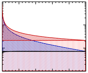
(a) Log–log plot of the DNS results for $I_1(\theta ) \equiv - \langle \bar {S}^{\sqrt \theta }_{ik} \bar {S}^{\sqrt \theta }_{kj} \bar {S}^{\sqrt {2\ell ^2-\theta }}_{ji} \rangle$, $I_2(\theta ) \equiv \langle \bar {\varOmega }^{\sqrt \theta }_{ik} \bar {\varOmega }^{\sqrt \theta }_{kj} \bar {S}^{\sqrt {2\ell ^2-\theta }}_{ji} \rangle$ and $I_4(\theta ) \equiv \langle \bar {\varOmega }^{\sqrt \theta }_{ik} \bar {S}^{\sqrt \theta }_{kj} \bar {\varOmega }^{\sqrt {2\ell ^2-\theta }}_{ji} \rangle$. (b) Same data as (a) but in a semi-log plot, with indications for the correspondence between several flux terms and the area of regions in the plot. The red shaded curved triangle, blue shaded curved triangle, red shaded rectangle, blue shaded rectangle and black area correspond to $\langle \varPi ^\ell _{nl,S} \rangle$, $\langle \varPi ^\ell _{nl,\varOmega } \rangle$, $\langle \varPi ^\ell _{l,S} \rangle$, $\langle \varPi ^\ell _{l,\varOmega } \rangle$ and $(\langle \varPi ^\ell _{nl,\varOmega } \rangle - \langle \varPi ^\ell _{nl,S} \rangle )/2$, respectively.

Note that in figure 2 the $I_4(\theta )$ curve is nearly independent of $\theta$, with a very slight decrease when $\theta /\eta ^2 \lesssim 10^3$, which turns out to have interesting dynamic consequences. Johnson (Reference Johnson2020) decomposed $\varPi ^\ell _S$ and $\varPi ^\ell _\varOmega$ into local and non-local parts: $\varPi ^\ell _S = \varPi ^\ell _{l,S} + \varPi ^\ell _{nl,S}$ and $\varPi ^\ell _\varOmega = \varPi ^\ell _{l,\varOmega } + \varPi ^\ell _{nl,\varOmega }$, where $\varPi ^\ell _{l,S} \equiv - \bar {S}^\ell _{ik} \bar {S}^\ell _{kj} \bar {S}^\ell _{ji} \ell ^2$ and $\varPi ^\ell _{l,\varOmega } \equiv \bar {\varOmega }^\ell _{ik} \bar {S}^\ell _{kj} \bar {\varOmega }^\ell _{ji} \ell ^2$. The DNS results show that $\langle \varPi ^\ell _{nl,S} \rangle$ is very close to $\langle \varPi ^\ell _{nl,\varOmega } \rangle$. Since $\langle \varPi ^\ell _{l,S} \rangle = - \langle \bar {S}^\ell _{ik} \bar {S}^\ell _{kj} \bar {S}^\ell _{ji} \rangle \ell ^2 = I_1(\ell ^2) \ell ^2$, this means that the local contribution $\langle \varPi ^\ell _S \rangle$ simply equals the area of the red rectangle shown in figure 2(b). Similarly, $\langle \varPi ^\ell _{l,\varOmega } \rangle = - \langle \bar {\varOmega }^\ell _{ik} \bar {S}^\ell _{kj} \bar {\varOmega }^\ell _{ji} \rangle \ell ^2 = I_2(\ell ^2) \ell ^2$ and corresponds to the area of the blue rectangle. The non-local contributions $\langle \varPi ^\ell _{nl,S} \rangle$ and $\langle \varPi ^\ell _{nl,\varOmega } \rangle$ correspond to the areas of the red and blue curved triangles. The difference between $\langle \varPi ^\ell _{nl,S} \rangle$ and $\langle \varPi ^\ell _{nl,\varOmega } \rangle$ is

(4.1)\begin{align} \varPi^\ell_{nl,S} - \varPi_{nl,\varOmega}^\ell & = (\varPi^\ell_S - \varPi^\ell_{l,S}) - (\varPi^\ell_\varOmega - \varPi^\ell_{l,\varOmega}) = (\varPi^\ell_S - \varPi^\ell_\varOmega) - ( \varPi^\ell_{l,S} - \varPi^\ell_{l,\varOmega}) \nonumber\\ & = 2 \int_0^{\ell^2} I_4(\theta) \, {\rm d} \theta - \ell^2 [I_1(\ell^2) - I_2(\ell^2) ] \nonumber\\ & \approx \ell^2 [ 2 I_4(\ell^2) - I_1(\ell^2) + I_2(\ell^2) ]= 0 , \end{align}

in which we used $I_4(\theta ) \approx {\rm const.} \approx I_4(\ell ^2)$ and the identity (3.12).

In figure 2, the other two terms, $I_1(\theta )$ and $I_2(\theta )$, grow rapidly as $\theta$ decreases towards $0$, and at $\theta = 0$, $I_1(0) \approx I_2(0) \gg I_4(0)$. To better understand this behaviour, we notice that for the isotropic case, (3.13) simplifies to $I_4(0) = \int _0^\infty \, {\rm d} r 4{\rm \pi} r^2 G_4(r) \mathscr {G}^{\sqrt 2 \ell }(r)$, where $G_4(r) = \langle \varOmega _{ik}(0) S_{kj}(0) \varOmega _{ji}(r) \rangle$, and similarly, $I_1(0) = \int _0^\infty \, {\rm d} r 4{\rm \pi} r^2 G_1(r) \mathscr {G}^{\sqrt 2 \ell }(r)$ and $I_2(0) = \int _0^\infty \, {\rm d} r 4{\rm \pi} r^2 G_2(r) \mathscr {G}^{\sqrt 2 \ell }(r)$, with $G_1(r) \equiv - \langle S_{ik}(0) S_{kj}(0) S_{ji}(r) \rangle$ and $G_2(r) \equiv \langle \varOmega _{ik}(0) \varOmega _{kj}(0) S_{ji}(r) \rangle$. In figure 3(a) we plot $G_1$, $G_2$ and $G_4$ as functions of $r$, normalized by their values at $r=0$. One can see that as $r$ increases, $G_4(r)$ decreases to $0$ much faster than $G_1$ and $G_2$, which results in $I_4(0) \ll I_1(0)$ and $I_2(0)$. In figure 3(b) we show the filtered version of G's in the HIT case, i.e. $G^{\sqrt \theta }_1(r) \equiv - \langle \bar {S}^{\sqrt \theta }_{ik}(0) \bar {S}^{\sqrt \theta }_{kj}(0) \bar {S}^{\sqrt \theta }_{ji}(r) \rangle$, $G^{\sqrt \theta }_2(r) \equiv \langle \bar {\varOmega }^{\sqrt \theta }_{ik}(0) \bar {\varOmega }^{\sqrt \theta }_{kj}(0) \bar {S}^{\sqrt \theta }_{ji}(r) \rangle$ and $G^{\sqrt \theta }_4(r) \equiv \langle \bar {\varOmega }^{\sqrt \theta }_{ik}(0) \bar {S}^{\sqrt \theta }_{kj}(0) \bar {\varOmega }^{\sqrt \theta }_{ji}(r) \rangle$. Those curves are qualitatively similar to those in figure 3(a); therefore, we still have $I_4(0) \ll I_1(0)$ and $I_2(0)$. In figures 3(a) and 3(b), the curves representing $G_1(r)$ and $G^{\sqrt \theta }_1(r)$ appear to be below those representing $G_2(r)$ and $G^{\sqrt \theta }_2(r)$ respectively and thus might raise the question as to whether indeed $I_1(\theta ) > I_2(\theta )$. This confusion is due to the fact that $G_i(r)$ shown in figure 3(a) and 3(b) were normalized by their corresponding values at $r=0$ and $G_i(0)$ differ in magnitude. In figures 3(c) and 3(d), the values of $G_i$ are plotted with non-dimensionalization by $G_1(0)$ or $G^{\sqrt \theta }_1(0)$, from which it is clearly seen that $G_1(r)$ and $G^{\sqrt \theta }_1(r)$ are above $G_2(r)$ and $G^{\sqrt \theta }_2(r)$ respectively. Thus we have $I_1(\theta ) \gtrsim I_2(\theta ) \gg I_4(\theta ) >0$, for $0 \leq \theta \leq \ell ^2$. In addition, we notice that the proof of (3.14) could also be applied to $G^{\sqrt \theta }_1$ and $G^{\sqrt \theta }_2$; thus all the $G$ curves should cross zero once and this is consistent with figure 3, although the negative values are minuscule and hard to see from the figure.

Figure 3.

(a) The DNS results for $G_1(r)/G_1(0)$ (blue lines), $G_2(r)/G_2(0)$ (red lines) and $G_4(r)/G_4(0)$ (magenta lines), with solid lines for $R_\lambda = 302$, dashed lines for $R_\lambda = 206$ and dot-dashed lines for $R_\lambda = 129$. (b) The DNS results for $G^{\sqrt \theta }_1(r)/G^{\sqrt \theta }_1(0)$, $G^{\sqrt \theta }_2(r)/G^{\sqrt \theta }_2(0)$ and $G^{\sqrt \theta }_4(r)/G^{\sqrt \theta }_4(0)$, the line designations being the same as in (a). (c) Same as (a) but all curves are normalized by $G_1(0)$. (d) Same as (b) but all curves are normalized by $G^{\sqrt \theta }_1(0)$.

Finally, we notice that the numerical results of Johnson (Reference Johnson2020) show that the magnitudes of SSA and VS are $\langle \varPi ^\ell _{S} \rangle : \langle \varPi ^\ell _{\varOmega }\rangle \approx 5 : 3$. Based on a simple K41-type scaling argument, our approach developed here leads to an approximate estimate of this ratio, namely $\langle \varPi ^\ell _{S} \rangle : \langle \varPi ^\ell _{\varOmega }\rangle \approx 9 : 5$, as shown in detail in the Appendix. The quantitative deviation of the model prediction from the DNS results indicates that the simple scaling analysis is not enough to describe the third-order moments of filtered velocity gradient.

5. Concluding remarks

In summary, we showed that in the filtered energy equation, the three contributions to the mean inter-scale energy transfer from SSA, VS and the correlation between strain and vorticity can all be expressed as integrals of third-order moments of filtered velocity gradients associated with two different filter sizes (equation (3.10)). With the help of that representation, and a relation involving third-order moments of filtered velocity gradients in homogeneous flows (equation (3.11)), we explained the observation that SSA dominates VS in kinetic energy transfer (Johnson Reference Johnson2020). Although the analytical results were compared with DNS of HIT, the derivation presented in this work is not restricted to HIT and could be applied to any homogeneous flows. Furthermore, the homogeneity constraint (equation (3.11)) provides an explanation to the observed nearly equal contributions from multi-scale strain amplification and VS (see figure 2b). We notice that those third-order moments of filtered velocity gradient (i.e. $I_1$ to $I_4$ in the text) could not be described by simple scaling analysis. Thus in the future it would be interesting to quantitatively investigate their properties, especially their roles in inter-scale energy transfer. Also, DNS of homogeneous but anisotropic turbulence could be used to verify the theoretical arguments in this work.