1 Introduction
Slender geometries are quite common in the realm of low Reynolds number fluid mechanics. Many microorganisms such as E. coli (Berg & Anderson Reference Berg and Anderson1973), Chlamydomonas (Bray Reference Bray2000), Paramecium (Brennen & Winet Reference Brennen and Winet1977) or human spermatozoa (Suarez & Pacey Reference Suarez and Pacey2006) use slender appendages to navigate through viscous fluid environments. The orientation distribution of plankton, some of which have elongated geometries, in the ocean is known to strongly influence the propagation of light in the deeper levels which can significantly influence the global carbon fixation (Guasto, Rusconi & Stocker Reference Guasto, Rusconi and Stocker2012). Slender particles such as fibres are used to make fibre-reinforced composites that have enhanced tensile strength and increased anisotropic thermal conductivity (Tekce, Kumlutas & Tavman Reference Tekce, Kumlutas and Tavman2007). Slender body theory (Batchelor Reference Batchelor1970; Cox Reference Cox1970; Keller & Rubinow Reference Keller and Rubinow1976; Johnson Reference Johnson1980) provides a computationally inexpensive route to study the dynamics of slender particles in highly viscous flows. However, the influence of the force per unit length generated by the gradient in the imposed fluid velocity has not been previously embedded in this theory.
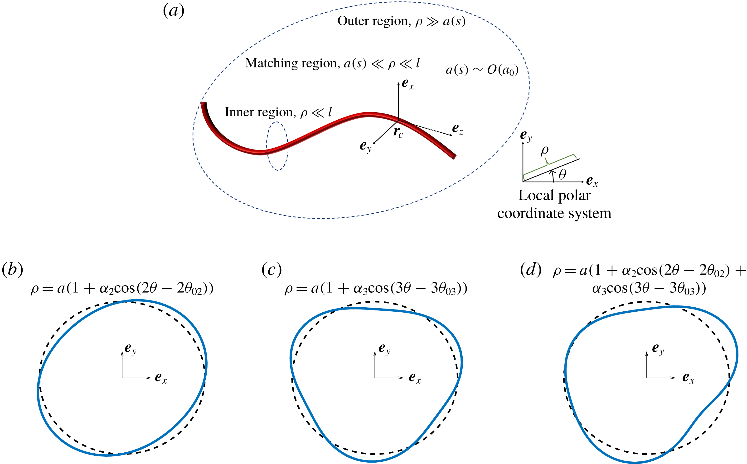
The force per unit length experienced by a slender filament with a circular cross-section at low Reynolds number, to leading order, is qualitatively similar to the viscous drag experienced by a long circular cylinder due to its relative motion with the local fluid velocity. Here, the existence of an additional force per unit length driven by the gradient in the imposed fluid velocity and its dependence on the shape of the cross-section is elucidated. In this study, the nature of the velocity disturbance is understood using a regular perturbation of the inner solution of the slender body theory (SBT) formulation. An integral equation is derived for the force per unit length experienced by the slender filament along with its dependence on the cross-sectional geometry. The force per unit length due to the non-circularity of the cross-section, has two components, one which is driven by the gradient in the imposed fluid velocity affecting three-lobed cross-sections (figure 1 c) and another driven by the motion of the particle relative to the fluid affecting two-lobed cross-sections (figure 1 b), a component first presented by Batchelor (Reference Batchelor1970). The additional force per unit length driven by the gradient in the fluid velocity is extremely important in the SBT formulation especially for computing the dynamics and rheology of thin particles in a linear flow field. A numerical calculation of the inner solution in a two-dimensional domain is proposed to extend our SBT formulation to particles with a general cross-sectional shape.
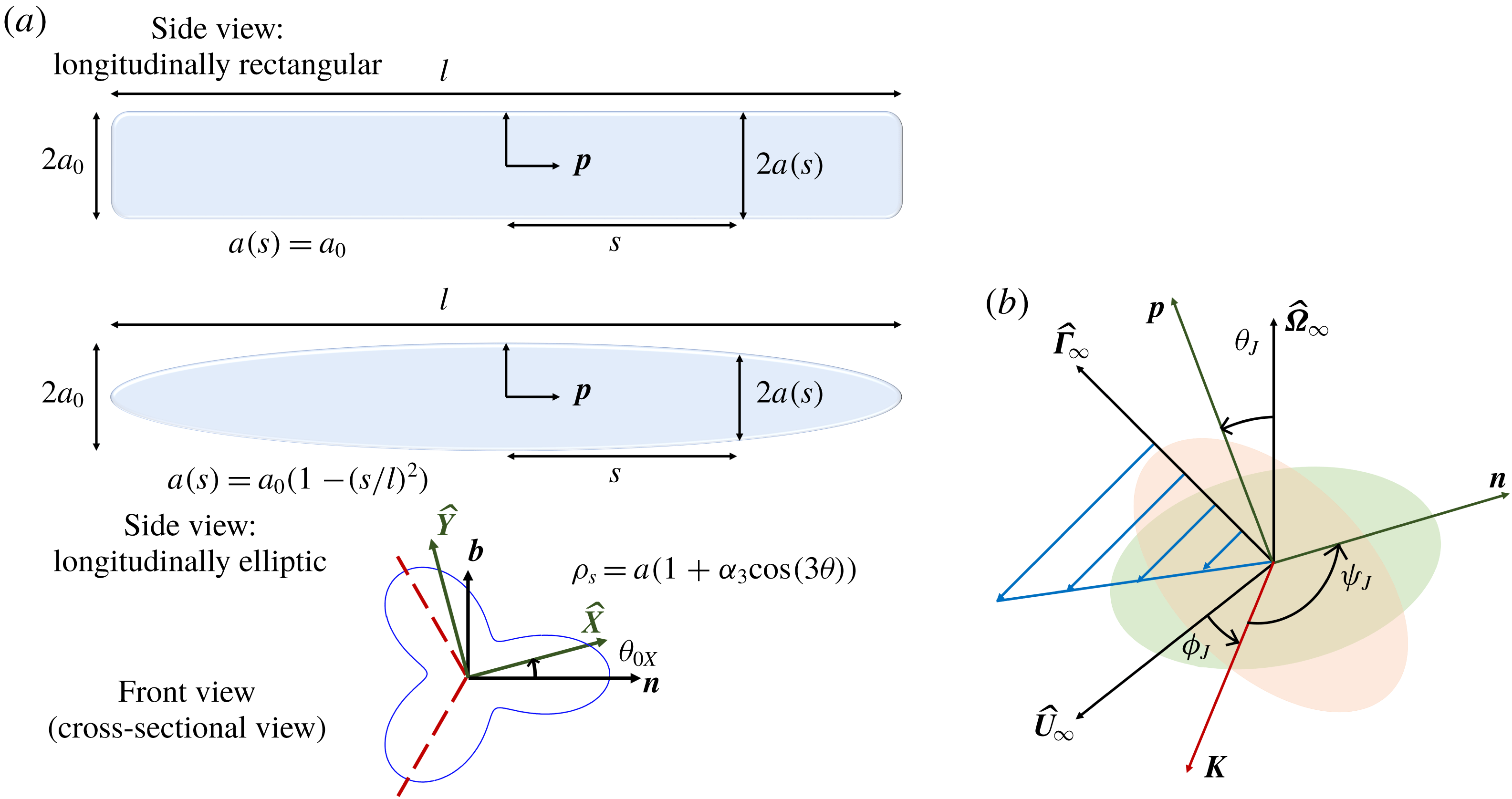
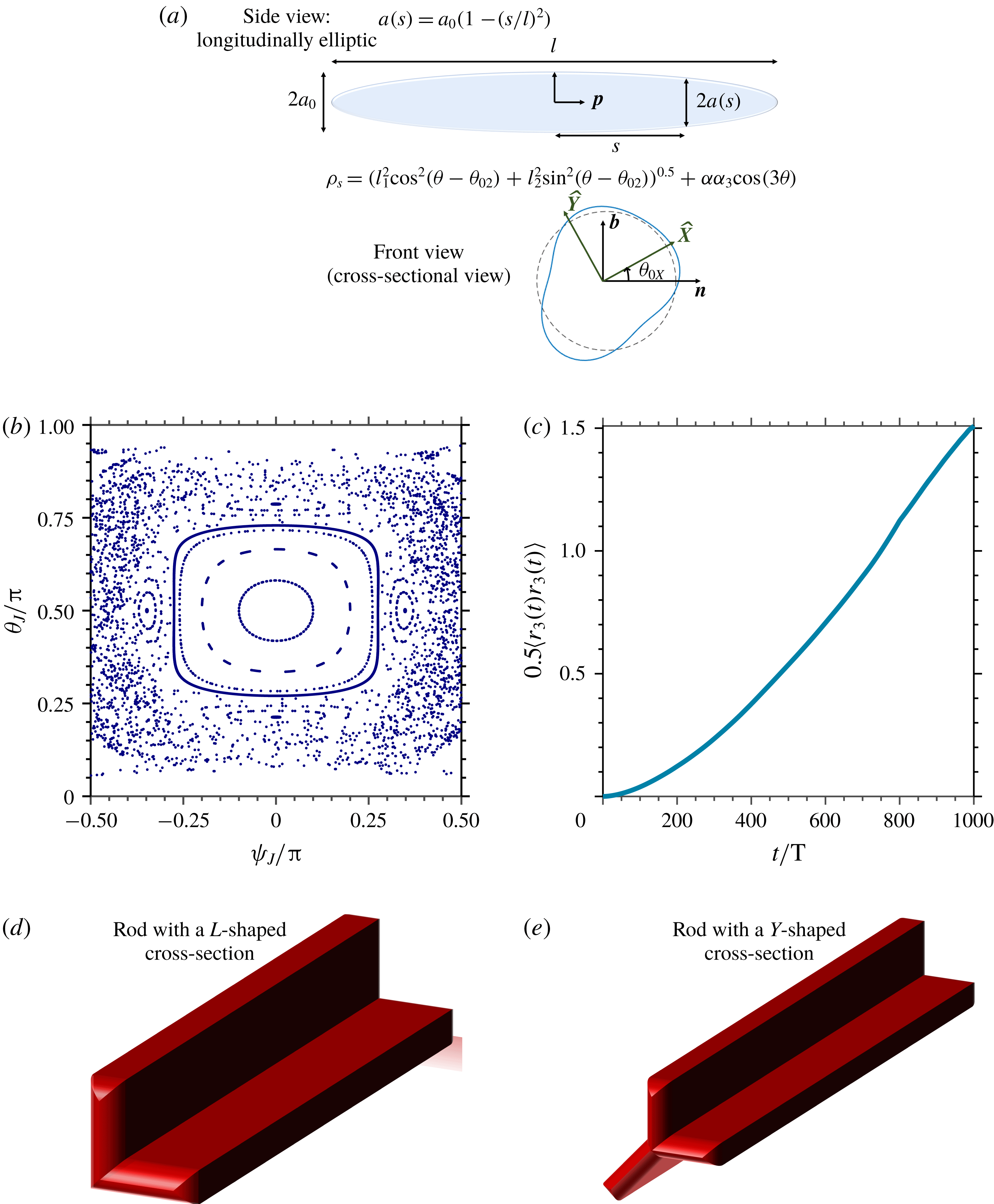
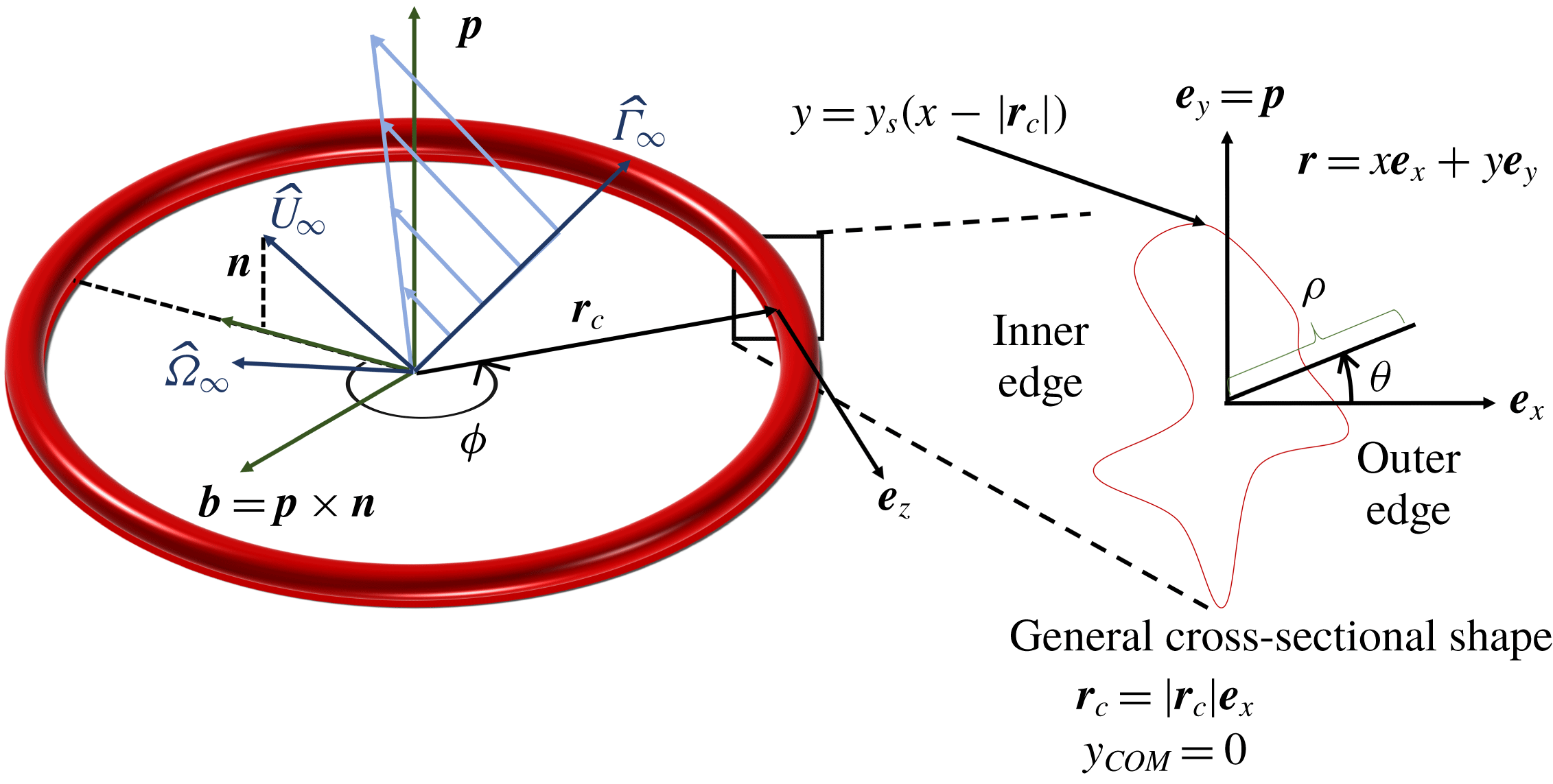
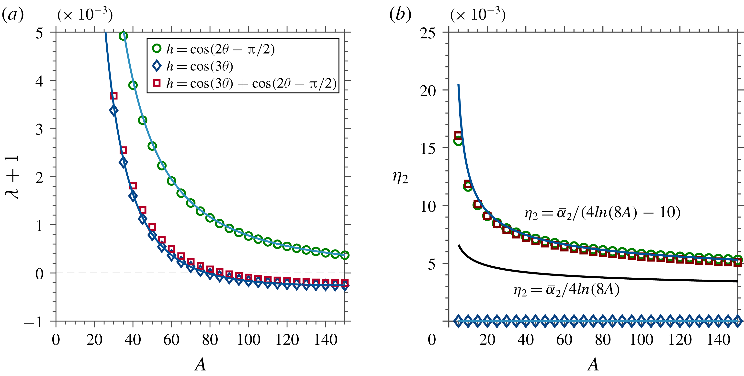
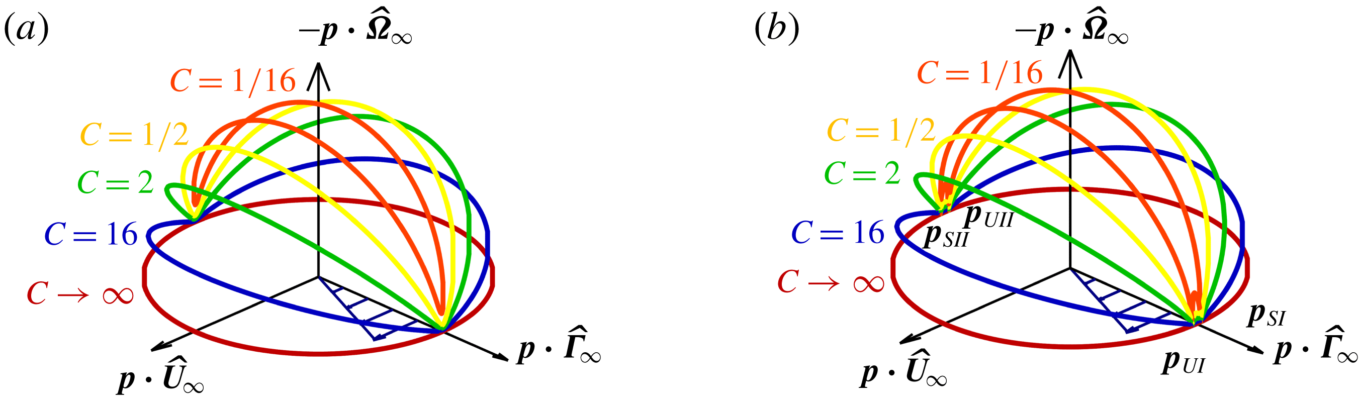
Local coordinate systems in the particle reference frame and the perturbed cross-sectional shapes studied here. (a) Local coordinate system for a general curved body;
 $\boldsymbol{e}_{\boldsymbol{z}}$
is along the tangent to the filament axis,
 $\boldsymbol{e}_{\boldsymbol{x}}$
is along the normal and
 $\boldsymbol{e}_{\boldsymbol{y}}$
is pointed along the binormal to the centreline of the slender body (
 $\boldsymbol{r}_{\boldsymbol{c}}$
). (b) Schematic of a two-lobed shape (S-I), given by
 $\unicode[STIX]{x1D70C}=a(1+\unicode[STIX]{x1D6FC}_{2}\cos (2\unicode[STIX]{x1D703}-2\unicode[STIX]{x1D703}_{02}))$
. (c) Schematic of a three-lobed shape (S-II), given by
 $\unicode[STIX]{x1D70C}=a(1+\unicode[STIX]{x1D6FC}_{3}\cos (3\unicode[STIX]{x1D703}-3\unicode[STIX]{x1D703}_{03}))$
. (d) Schematic of a shape, which is a linear combination of the two- and three-lobed perturbations, given by
 $\unicode[STIX]{x1D70C}=a(1+\unicode[STIX]{x1D6FC}_{2}\cos (2\unicode[STIX]{x1D703}-2\unicode[STIX]{x1D703}_{02})+\unicode[STIX]{x1D6FC}_{3}\cos (3\unicode[STIX]{x1D703}-3\unicode[STIX]{x1D703}_{03}))$
(S-III shape). ‘
 $a$
’ the radius of the equivalent circle is allowed to vary along the centreline of the filament.

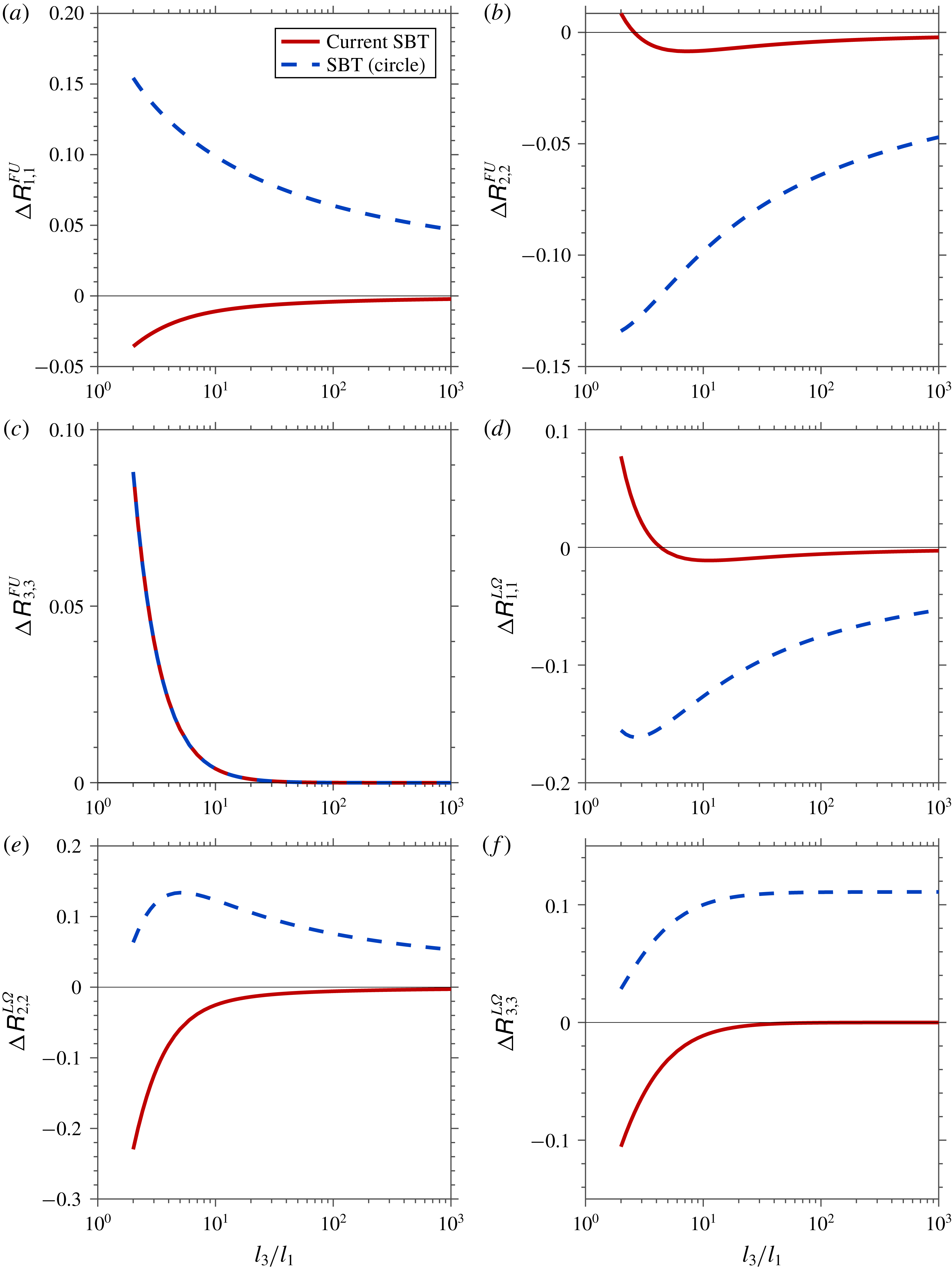
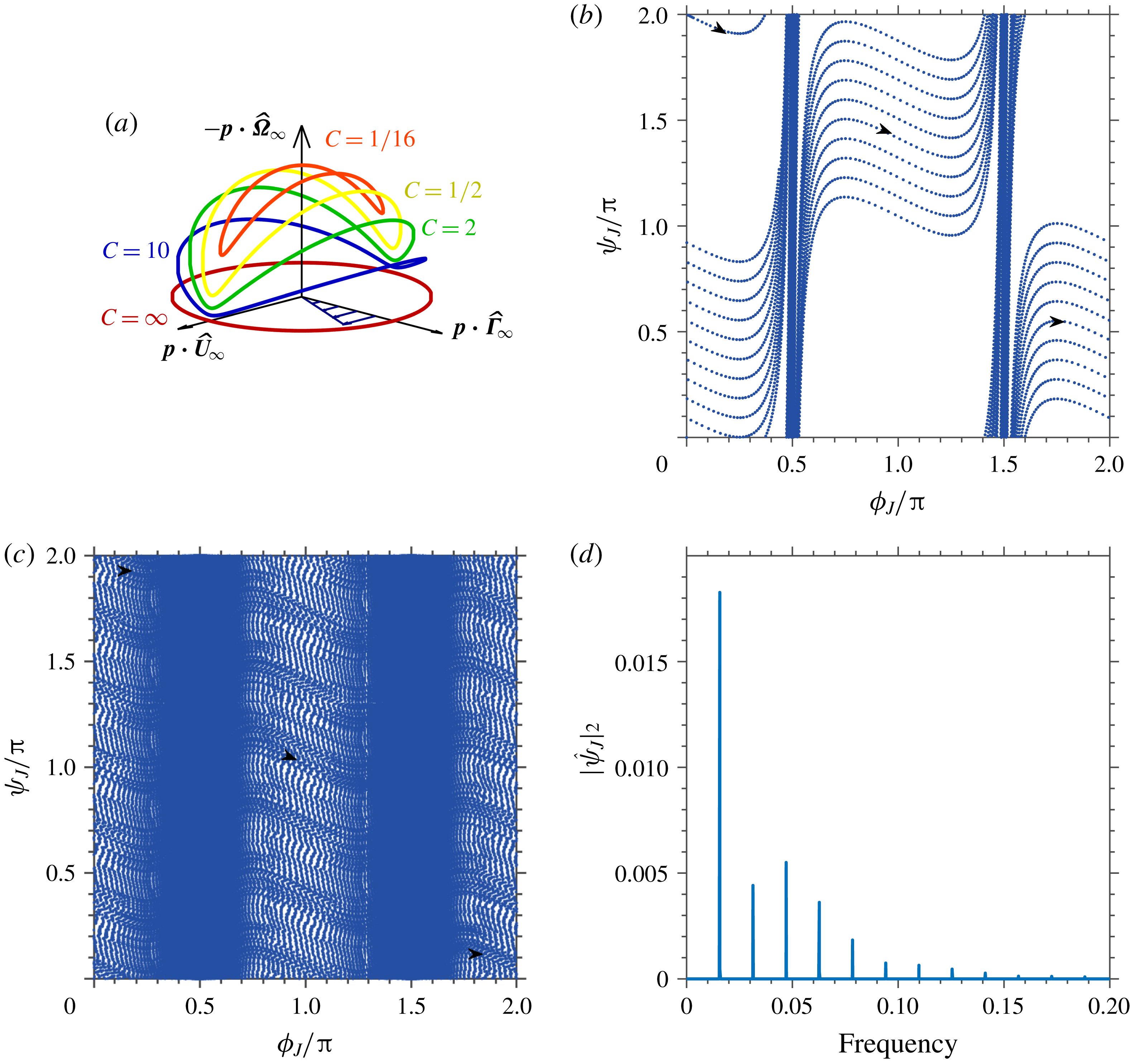
The current theory accurately predicts the resistance to rotation and translation of slender triaxial ellipsoids retaining accuracy even when the cross-section has a high aspect ratio (§ 4). In § 5, straight particles with three-lobed cross-sections, illustrated in figure 1(c), are shown to rotate and translate quasi-periodically in a simple shear flow (SSF) because of the force per unit length driven by the imposed velocity gradient. In contrast, a straight particle with a combination of a two- and a three-lobed cross-section, shown in figure 1(d), can diffuse in space while rotating chaotically. This work allows for the inclusion of these dynamics which can potentially impact the rheology of a suspension of straight particles. In § 6, our theory is utilized to predict the dynamics of rings with non-circular cross-section, and the results remain accurate for cross-sections that deviate significantly from a circle or have aspect ratios as low as 10.
Slender body theory (SBT) allows for an approximate solution of the governing equation modelling a physical phenomenon that is affected by the presence of bodies which are long and thin. The governing equations of highly viscous flows (Stokes flow), potential flows and heat transfer have been solved using the SBT formulation for many applications. Potential flow problems that include animal locomotion (Lighthill Reference Lighthill1960, Reference Lighthill1971), force on airship hulls (Munk Reference Munk1924), force on wings (Jones Reference Jones1946) and ship hydrodynamics (Newman Reference Newman1964, Reference Newman1970) have been solved using SBT. Steady state heat transfer in composites (Rocha & Acrivos Reference Rocha and Acrivos1973a ,Reference Rocha and Acrivos b ; Chen & Acrivos Reference Chen and Acrivos1976; Acrivos & Shaqfeh Reference Acrivos and Shaqfeh1988; Shaqfeh Reference Shaqfeh1988; Fredrickson & Shaqfeh Reference Fredrickson and Shaqfeh1989; Mackaplow, Shaqfeh & Schiek Reference Mackaplow, Shaqfeh and Schiek1994) and transient heat transfer in ground-source heat pumps (Beckers, Koch & Tester Reference Beckers, Koch and Tester2015) are a few applications of SBT for steady state and transient heat conduction respectively. In the realm of highly viscous flows, problems involving flagellar hydrodynamics (Johnson & Brokaw Reference Johnson and Brokaw1979), structure and rheology of fibre suspensions (Rahnama et al. Reference Rahnama, Koch, Iso and Cohen1993; Rahnama, Koch & Shaqfeh Reference Rahnama, Koch and Shaqfeh1995; Mackaplow & Shaqfeh Reference Mackaplow and Shaqfeh1996, Reference Mackaplow and Shaqfeh1998) and separation of racemic mixtures of screw shaped particles (Kim & Rae Reference Kim and Rae1991) have been solved using existing SBT techniques for Stokes flow (Batchelor Reference Batchelor1970; Cox Reference Cox1970; Keller & Rubinow Reference Keller and Rubinow1976; Johnson Reference Johnson1980).
The basic idea in SBT is to obtain the strength of a line of singularities placed along the centreline of the slender filament that approximates the field of interest around the filament far away from the cross-sectional surface, termed as the outer region, i.e.
 $a\ll \unicode[STIX]{x1D70C}$
. Here
 $\unicode[STIX]{x1D70C}$
is the radial distance from the centreline of the slender filament, and ‘
 $a$
’ is a measure of the cross-sectional size of the particle at a certain location along the centreline of the slender body as shown in figure 1(a). The singularity for a potential flow problem is a point source of mass, for a heat transfer problem a point source of heat and for a Stokes flow problem a point force. The strength of the singularities is found by matching the field approximated in the outer region, termed as the outer solution, to a field obtained from the inner region (i.e.
 $\unicode[STIX]{x1D70C}\ll l$
, where
 $l$
is the length of the slender filament). Placing higher-order singularities along the centreline of the slender filament gives a better estimate of the field of interest. For a Stokes flow problem, which is the main topic of discussion in this paper, these singularities would include doublets, rotlets, sources, stresslets and quadrupoles (Johnson Reference Johnson1980).
In Stokes flow, the force per unit length exerted by the body on the fluid (i.e. the strength of the singularity) is derived at each point along the centreline of the slender body in terms of the motion of the particle and the imposed fluid velocity. The length, ‘
 $l$
’, an appropriate velocity and the fluid viscosity are used to non-dimensionalize all variables throughout this paper unless mentioned otherwise. The force per unit length exerted by a slender body on the fluid, which is due to relative motion of the particle, and fluid, can be expressed as a series in
 $\unicode[STIX]{x1D716}=1/\ln (2A)$
(Batchelor Reference Batchelor1970; Cox Reference Cox1970), where
 $A=l/(a_{0})$
is the aspect ratio of the particle and
 $a_{0}$
is the characteristic value of
 $a(s)$
. The first term in this series arises only due to the local relative velocity between the particle and the fluid and is
 $O(\unicode[STIX]{x1D716})$
(Batchelor Reference Batchelor1970; Cox Reference Cox1970). Cox (Reference Cox1970) was the first to demonstrate that the force per unit length is affected at
 $O(\unicode[STIX]{x1D716}^{2})$
by the centreline curvature (see equations (6.2) and (6.3) of his paper). Keller & Rubinow (Reference Keller and Rubinow1976) gave an integral equation for the force per unit length which can be iteratively solved to obtain higher-order corrections to the force per unit length with errors of
 $O(\unicode[STIX]{x1D716}^{N})$
, where
 $N$
is an integer such that
 $N\geqslant 2$
. Johnson (Reference Johnson1980) produced an integral equation for the force per unit length with errors of
 $O(1/A^{2})$
which also included the effects of the ends of the slender body (equation (19) of his paper). Johnson (Reference Johnson1980) also described a method to incorporate the effect of centreline curvature in the inner solution (equation (31) of his paper).
Batchelor (Reference Batchelor1970) showed that the cross-sectional shape of the particle first affects the force per unit length at
 $O(\unicode[STIX]{x1D716}^{2})$
, the same order of importance as the centreline curvature of the body. Batchelor (Reference Batchelor1970) described how the force per unit length for an arbitrary cross-section can be found by solving for the longitudinal velocity field due to an equivalent circle of a certain radius, and the transverse velocity field due to an equivalent ellipse of certain dimensions and orientation. Batchelor (Reference Batchelor1954) provided the method to obtain the equivalent circular cylinder by solving the harmonic equation for the flow along the longitudinal direction. Batchelor (Reference Batchelor1970) described the procedure to obtain an equivalent ellipse by solving the biharmonic equation for the velocity field in the transverse plane around the cross-sectional shape in question.
Cox (Reference Cox1971) was the first to account for the effect of the gradient in the imposed velocity of a linear flow field on the force and torque acting on a slender cylinder with tapered ends, which was oriented such that the imposed velocity field at the particle centreline is exactly zero. Cox placed a force and dipole per unit length along the centreline of the body to approximate the velocity field in the outer region, while Keller & Rubinow (Reference Keller and Rubinow1976) employed a stresslet and rotlet per unit length for the same purpose. Singh et al. (Reference Singh, Koch, Subramanian and Stroock2014) discuss the equivalence of these two formulations by showing that the variation of the force per unit length leads to a net stresslet and a rotlet on a slice of the particle. The rotlet per unit length can lead to a finite torque on the particle whereas a variable stresslet per unit length, which occurs when the particle cross-section varies along the longitudinal direction, can lead to a finite force acting on the particle of
 $O(\unicode[STIX]{x1D716}^{2}/A^{2})$
. A straight circular cylinder with a constant cross-section cannot experience a force per unit length at this orientation if the cross-section is circular. However, the force per unit length due to the velocity gradient can be non-zero if the cross-section is non-circular. This force per unit length, which will be
 $O(\unicode[STIX]{x1D716}/A)$
as explained in § 3, can lead to a net force of
 $O(\unicode[STIX]{x1D716}/A)$
acting on the particle.
In this paper, the additional
 $O(\unicode[STIX]{x1D716}/A)$
contribution to the force per unit length in addition to Batchelor’s correction of
 $O(\unicode[STIX]{x1D716}^{2})$
is derived in § 3. This calculation is especially important when considering motion of force and torque-free slender particles in SSF. In such scenarios, Batchelor’s correction tends to zero for certain particle orientations, while Cox’s (Reference Cox1971) correction predicts a much smaller effect on the particle rotation rate. Thus, both previous theories lead to an incorrect qualitative behaviour for particle geometries such as straight cylinders with elliptic cross-sections (Yarin, Gottlieb & Roisman Reference Yarin, Gottlieb and Roisman1997) or rings with three-lobed cross-sections (Singh, Koch & Stroock Reference Singh, Koch and Stroock2013) in SSF.
2 SBT solution for circular cross-section
In this section, the velocity disturbance created by a slender particle with a circular cross-section, when placed in a fluid moving with a velocity
 $\boldsymbol{u}_{\boldsymbol{\infty }}$
in the absence of the particle is described. This calculation will be used to obtain the effect of the cross-sectional shape in § 3. The slenderness parameter or the aspect ratio (
 $A=l/(a_{0})$
), is defined as the ratio of the half-length of the filament (
 $l$
) and a measure of the radius of the cross-section (
 $a_{0}$
). The radius of the cross-section,
 $a\sim O(a_{0})$
, is allowed to vary along the longitudinal direction of the slender body. The position vector is denoted by
 $\boldsymbol{r}$
and
 $\boldsymbol{r}_{\boldsymbol{c}}$
denotes the position of the centreline of the slender filament. A local coordinate system (
 $\boldsymbol{e}_{\boldsymbol{x}},\boldsymbol{e}_{\boldsymbol{y}},\boldsymbol{e}_{\boldsymbol{z}}$
) is chosen based on the tangent (
 $\boldsymbol{e}_{\boldsymbol{z}}$
), normal (
 $\boldsymbol{e}_{\boldsymbol{x}}$
) and binormal (
 $\boldsymbol{e}_{\boldsymbol{y}}$
) to the centreline of the slender body, as shown in figure 1(a), and is mathematically given by
 $$\begin{eqnarray}\boldsymbol{e}_{\boldsymbol{z}}=\frac{\unicode[STIX]{x2202}\boldsymbol{r}_{\boldsymbol{C}}}{\unicode[STIX]{x2202}s},\quad \boldsymbol{e}_{\boldsymbol{x}}=\frac{1}{\unicode[STIX]{x1D705}}\frac{\unicode[STIX]{x2202}^{2}\boldsymbol{r}_{\boldsymbol{C}}}{\unicode[STIX]{x2202}s^{2}},\quad \boldsymbol{e}_{\boldsymbol{y}}=\boldsymbol{e}_{\boldsymbol{z}}\times \boldsymbol{e}_{\boldsymbol{x}},\end{eqnarray}$$
where ‘
 $s$
’ denotes the arc length along the centreline and
 $\unicode[STIX]{x1D705}$
is the local curvature of the body centreline. A local polar coordinate system (
 $\unicode[STIX]{x1D70C}$
–
 $\unicode[STIX]{x1D703}$
), as shown in figure 1(a), is defined in the
 $\boldsymbol{e}_{\boldsymbol{x}}$
–
 $\boldsymbol{e}_{\boldsymbol{y}}$
plane, where
 $\unicode[STIX]{x1D703}$
is measured from
 $\boldsymbol{e}_{\boldsymbol{x}}$
and
 $\unicode[STIX]{x1D70C}$
is the normal distance from the centreline. The far-field fluid velocity is denoted by
 $\boldsymbol{u}_{\boldsymbol{\infty }}$
, which is allowed to vary with
 $\boldsymbol{r}$
. The velocity on the particle surface (
 $\boldsymbol{r}=\boldsymbol{r}_{\boldsymbol{s}}$
) is given by
 $$\begin{eqnarray}\boldsymbol{u}(\boldsymbol{r}=\boldsymbol{r}_{\boldsymbol{s}})=\boldsymbol{U}+\unicode[STIX]{x1D74E}\times \boldsymbol{r}_{\boldsymbol{s}}=(\boldsymbol{U}+\unicode[STIX]{x1D74E}\times \boldsymbol{r}_{\boldsymbol{c}})+\unicode[STIX]{x1D74E}\times (\boldsymbol{r}_{\boldsymbol{s}}-\boldsymbol{r}_{\boldsymbol{c}}),\end{eqnarray}$$
where
 $\boldsymbol{U}$
and
 $\unicode[STIX]{x1D74E}$
are the particle velocity at the origin (
 $\boldsymbol{r}=\mathbf{0}$
) and angular velocity of the particle, respectively. These definitions are valid for any cross-sectional shape. The rest of this section describes the slender body theory solution for a circular cross-section of radius ‘
 $a$
’. The force per unit length and all the unknown constants in the inner solution, which are required for the perturbation analysis in § 3, are obtained in this section.
2.1 Velocity field in the inner region
 $(\unicode[STIX]{x1D70C}\ll 1)$

Any curved slender body with
 $O(1)$
curvature appears locally as a straight infinite cylinder to a first approximation. The velocity field in the inner region is obtained by assuming flow over an infinite cylinder. Thus, the flow along and transverse to the cylinder is solved separately. Any coupling between these flows arises due to curvature and finite aspect ratio of the particle and leads to algebraic
 $O(1/A^{2})$
corrections to the velocity disturbance (Johnson Reference Johnson1980) which are not discussed here. The functional form of the flow in the transverse plane is obtained by solving a two-dimensional Stokes flow problem that satisfies the no-slip condition on the particle surface. The far-field boundary condition is applied later while asymptotically matching the velocity fields from the inner and outer regions to obtain any unknowns. The solution to the biharmonic equation (
 $\unicode[STIX]{x1D6FB}^{4}\unicode[STIX]{x1D713}=0$
) is used to obtain the functional form of the velocity field in the plane transverse to the slender dimension. The two-dimensional velocity field is obtained from the definition of the streamfunction, i.e.
 $u_{\unicode[STIX]{x1D70C}}=\unicode[STIX]{x1D70C}^{-1}\,\text{d}\unicode[STIX]{x1D713}/\text{d}\unicode[STIX]{x1D703}$
and
 $u_{\unicode[STIX]{x1D703}}=-\,\text{d}\unicode[STIX]{x1D713}/\text{d}\unicode[STIX]{x1D70C}$
. The solution around a circular cross-section of radius ‘
 $a$
’ in terms of the streamfunction (
 $\unicode[STIX]{x1D713}$
) in polar coordinates is given by
 $$\begin{eqnarray}\displaystyle \frac{\unicode[STIX]{x1D713}}{a} & = & \displaystyle \left(\frac{\tilde{\unicode[STIX]{x1D713}}}{a}\right)+[B\cos (\unicode[STIX]{x1D703})+\hat{B}\sin (\unicode[STIX]{x1D703})]\left[\left(\frac{\unicode[STIX]{x1D70C}}{a}\right)-\left(\frac{\unicode[STIX]{x1D70C}}{a}\right)^{-1}-2\ln \left(\frac{\unicode[STIX]{x1D70C}}{a}\right)\left(\frac{\unicode[STIX]{x1D70C}}{a}\right)\right]\nonumber\\ \displaystyle & & \displaystyle +\,[(\boldsymbol{U}+\unicode[STIX]{x1D74E}\times \boldsymbol{r}_{\boldsymbol{c}})\boldsymbol{\cdot }(\boldsymbol{e}_{\boldsymbol{x}}\sin (\unicode[STIX]{x1D703})-\boldsymbol{e}_{\boldsymbol{y}}\cos (\unicode[STIX]{x1D703}))]\left[\left(\frac{\unicode[STIX]{x1D70C}}{a}\right)^{-\mathbf{1}}+2\frac{\unicode[STIX]{x1D70C}}{a}\ln \left(\frac{\unicode[STIX]{x1D70C}}{a}\right)\right]\nonumber\\ \displaystyle & & \displaystyle -\,(\unicode[STIX]{x1D74E}\boldsymbol{\cdot }\boldsymbol{e}_{\boldsymbol{z}})a\ln \left(\frac{\unicode[STIX]{x1D70C}}{a}\right),\end{eqnarray}$$
where
 $\tilde{\unicode[STIX]{x1D713}}$
is the streamfunction that approaches the streamfunction of the imposed flow field for
 $\unicode[STIX]{x1D70C}\gg a$
, while satisfying the zero-velocity boundary condition on the particle surface.
 $B$
and
 $\hat{B}$
are obtained by matching this velocity field to the one from the outer region and depend on the force per unit length acting on the slender body, the imposed flow field and the particle velocities (
 $\boldsymbol{U}$
and
 $\unicode[STIX]{x1D74E}$
). The velocity in polar coordinates in the inner region is given by
 $$\begin{eqnarray}\displaystyle u_{\unicode[STIX]{x1D70C}} & = & \displaystyle \frac{1}{\unicode[STIX]{x1D70C}}\frac{\unicode[STIX]{x2202}\unicode[STIX]{x1D713}}{\unicode[STIX]{x2202}\unicode[STIX]{x1D703}}=\frac{1}{\unicode[STIX]{x1D70C}}\frac{\unicode[STIX]{x2202}\tilde{\unicode[STIX]{x1D713}}}{\unicode[STIX]{x2202}\unicode[STIX]{x1D703}}+[-B\sin (\unicode[STIX]{x1D703})+\hat{B}\cos (\unicode[STIX]{x1D703})]\left[1-\left(\frac{\unicode[STIX]{x1D70C}}{a}\right)^{-2}-2\ln \left(\frac{\unicode[STIX]{x1D70C}}{a}\right)\right]\nonumber\\ \displaystyle & & \displaystyle +\,[(\boldsymbol{U}+\unicode[STIX]{x1D74E}\times \boldsymbol{r}_{\boldsymbol{c}})\boldsymbol{\cdot }(\boldsymbol{e}_{\boldsymbol{x}}\cos (\unicode[STIX]{x1D703})+\boldsymbol{e}_{\boldsymbol{y}}\sin (\unicode[STIX]{x1D703}))]\left[\left(\frac{\unicode[STIX]{x1D70C}}{a}\right)^{-2}+2\ln \left(\frac{\unicode[STIX]{x1D70C}}{a}\right)\right],\end{eqnarray}$$
 $$\begin{eqnarray}\displaystyle u_{\unicode[STIX]{x1D703}} & = & \displaystyle -\frac{\unicode[STIX]{x2202}\unicode[STIX]{x1D713}}{\unicode[STIX]{x2202}\unicode[STIX]{x1D70C}}=-\frac{\unicode[STIX]{x2202}\tilde{\unicode[STIX]{x1D713}}}{\unicode[STIX]{x2202}\unicode[STIX]{x1D70C}}+[B\cos (\unicode[STIX]{x1D703})+\hat{B}\sin (\unicode[STIX]{x1D703})]\left[1-\left(\frac{\unicode[STIX]{x1D70C}}{a}\right)^{-2}+2\ln \left(\frac{\unicode[STIX]{x1D70C}}{a}\right)\right]\nonumber\\ \displaystyle & & \displaystyle +\,[(\boldsymbol{U}+\unicode[STIX]{x1D74E}\times \boldsymbol{r}_{\boldsymbol{c}})\boldsymbol{\cdot }(\boldsymbol{e}_{\boldsymbol{x}}\sin (\unicode[STIX]{x1D703})-\boldsymbol{e}_{\boldsymbol{y}}\cos (\unicode[STIX]{x1D703}))]\left[\left(\frac{\unicode[STIX]{x1D70C}}{a}\right)^{-2}-2-2\ln \left(\frac{\unicode[STIX]{x1D70C}}{a}\right)\right]\nonumber\\ \displaystyle & & \displaystyle +\,\unicode[STIX]{x1D74E}\boldsymbol{\cdot }\boldsymbol{e}_{\boldsymbol{z}}a\left(\frac{\unicode[STIX]{x1D70C}}{a}\right)^{-1}.\end{eqnarray}$$
The velocity along the longitudinal direction is obtained by assuming negligible change in pressure along the longitudinal direction (i.e.
 $\unicode[STIX]{x1D6FB}^{2}u_{z}=0$
). The velocity field along a slender filament with circular cross-section is given by
 $$\begin{eqnarray}u_{z}=\tilde{u} _{z}+E\ln \left(\frac{\unicode[STIX]{x1D70C}}{a}\right)+(\boldsymbol{U}+\unicode[STIX]{x1D74E}\times \boldsymbol{r}_{\boldsymbol{c}})\boldsymbol{\cdot }\boldsymbol{e}_{\boldsymbol{z}}+\left(\frac{\unicode[STIX]{x1D70C}}{a}\right)^{-1}(\unicode[STIX]{x1D74E}\boldsymbol{\cdot }\boldsymbol{e}_{\boldsymbol{ x}}a\sin (\unicode[STIX]{x1D703})-\unicode[STIX]{x1D74E}\boldsymbol{\cdot }\boldsymbol{e}_{\boldsymbol{y}}a\cos (\unicode[STIX]{x1D703})),\end{eqnarray}$$
where
 $\tilde{u} _{z}$
is the velocity field that approaches
 $\boldsymbol{u}_{\boldsymbol{\infty }}\boldsymbol{\cdot }\boldsymbol{e}_{\boldsymbol{z}}$
for
 $\unicode[STIX]{x1D70C}/a\gg 1$
, and equals zero on the particle surface,
 $E$
is obtained by matching the inner region velocity field to the outer solution and depends on the imposed flow field, the particle velocities (
 $\boldsymbol{U}$
and
 $\unicode[STIX]{x1D74E}$
) and the force per unit length on the filament. The overall error in (2.4)–(2.6) is the larger of
 $O(1/A^{2})$
and the order of errors in
 $B$
,
 $\hat{B}$
and
 $E$
, determined by matching the inner velocity field to the outer solution.
2.2 Velocity field in the outer region
$(\unicode[STIX]{x1D70C}\gg a(s))$

In the outer region, the velocity disturbance due to a slender filament is approximately captured by a suitable choice of Stokeslet distribution along the particle centreline (
 $\boldsymbol{r}_{\boldsymbol{c}}$
) (Cox Reference Cox1970). A Stokeslet is a point force solution to the Stokes equations. The velocity disturbance created by a line of force per unit length is given by
 $$\begin{eqnarray}\boldsymbol{u}(\boldsymbol{r})\approx \boldsymbol{u}_{\boldsymbol{\infty }}(\boldsymbol{r})+\frac{1}{8\unicode[STIX]{x03C0}}\int _{\boldsymbol{r}_{\boldsymbol{c}}}\,\text{d}s^{\prime }\left(\frac{\boldsymbol{I}}{|\boldsymbol{r}-\boldsymbol{r}^{\prime }|}+\frac{(\boldsymbol{r}-\boldsymbol{r}^{\prime })(\boldsymbol{r}-\boldsymbol{r}^{\prime })}{|\boldsymbol{r}-\boldsymbol{r}^{\prime }|^{3}}\right)\boldsymbol{\cdot }\boldsymbol{f}(\boldsymbol{r}^{\prime }),\end{eqnarray}$$
where
 $\boldsymbol{r}$
is the point at which the velocity is evaluated,
 $\boldsymbol{r}^{\prime }$
takes all values along the centreline and
 $\text{d}s^{\prime }$
is the elemental length along the centreline of the slender body. Equation (2.7) has errors of
 $O(1/A^{2})$
. As
 $\boldsymbol{r}^{\prime }\rightarrow \boldsymbol{r}$
, the integrand in (2.7) diverges as
 $\ln (\unicode[STIX]{x1D70C})$
. This diverging part of the integral in (2.7) is separated from the rest of the integral as shown by Keller & Rubinow (Reference Keller and Rubinow1976) and the resulting equation for
 $\unicode[STIX]{x1D70C}\ll 1$
is given by
 $$\begin{eqnarray}\displaystyle \boldsymbol{u}(\boldsymbol{r}) & {\approx} & \displaystyle \boldsymbol{u}_{\boldsymbol{\infty }}(\boldsymbol{r})-\frac{1}{4\unicode[STIX]{x03C0}}(\boldsymbol{I}+\boldsymbol{e}_{\boldsymbol{z}}\boldsymbol{e}_{\boldsymbol{z}})\boldsymbol{\cdot }\boldsymbol{f}(\boldsymbol{r})\left[\ln \left(\frac{\unicode[STIX]{x1D70C}}{2}\right)-\ln \left(\frac{s(1-s)}{a(s)}\right)\right]-\frac{1}{4\unicode[STIX]{x03C0}}\boldsymbol{f}\boldsymbol{\cdot }\boldsymbol{e}_{\boldsymbol{z}}\boldsymbol{e}_{\boldsymbol{z}}\nonumber\\ \displaystyle & & \displaystyle +\,\frac{1}{4\unicode[STIX]{x03C0}}\boldsymbol{f}\boldsymbol{\cdot }\boldsymbol{e}_{\unicode[STIX]{x1D70C}}\boldsymbol{e}_{\unicode[STIX]{x1D70C}}+\frac{1}{8\unicode[STIX]{x03C0}}\int _{\boldsymbol{r}_{\boldsymbol{c}}}\,\text{d}s^{\prime }\left[\left(\frac{\boldsymbol{I}}{|\boldsymbol{r}_{\boldsymbol{c}}(s)-\boldsymbol{r}_{\boldsymbol{c}}(s^{\prime })|}+\frac{(\boldsymbol{r}_{\boldsymbol{c}}(s)-\boldsymbol{r}_{\boldsymbol{c}}(s^{\prime }))(\boldsymbol{r}_{\boldsymbol{ c}}(s)-\boldsymbol{r}_{\boldsymbol{c}}(s^{\prime }))}{|\boldsymbol{r}_{\boldsymbol{c}}(s)-\boldsymbol{r}_{\boldsymbol{c}}(s^{\prime })|^{3}}\right)\right.\nonumber\\ \displaystyle & & \displaystyle \boldsymbol{\cdot }\left.\boldsymbol{f}(\boldsymbol{r}^{\prime })-\left(\frac{\boldsymbol{I}}{|s-s^{\prime }|}+\frac{\boldsymbol{e}_{\boldsymbol{z}}\boldsymbol{e}_{\boldsymbol{z}}}{|s-s^{\prime }|}\right)\boldsymbol{\cdot }\boldsymbol{f}(\boldsymbol{r})\right],\end{eqnarray}$$
where
 $\boldsymbol{e}_{\unicode[STIX]{x1D70C}}$
is the radial vector in the
 $\boldsymbol{e}_{\boldsymbol{x}}$
–
 $\boldsymbol{e}_{\boldsymbol{y}}$
plane. The integral on the right-hand side of (2.8) is shown to have a finite limit by Keller & Rubinow (Reference Keller and Rubinow1976). The
 $\ln (\unicode[STIX]{x1D70C})$
term in (2.8), matches the
 $\ln (\unicode[STIX]{x1D70C})$
of the inner solution in (2.4)–(2.6) and also corresponds to the velocity disturbance produced by an infinite cylinder with the same force per unit length at each point.
2.3 Matching region
$(a\ll \unicode[STIX]{x1D70C}\ll 1)$

The velocity produced from the inner solution for
 $\unicode[STIX]{x1D70C}\gg a$
, should asymptotically match the velocity field from the outer solution for
 $\unicode[STIX]{x1D70C}\ll 1$
as the velocity field cannot abruptly change in this matching region (i.e.
 $a\ll \unicode[STIX]{x1D70C}\ll 1$
). Matching the velocity fields from the inner and outer solutions, using (2.4)–(2.6) and (2.8), yields the constants in the inner solution,
 $\hat{B}=(\boldsymbol{U}+(\unicode[STIX]{x1D74E}\times \boldsymbol{r}_{\boldsymbol{c}}))\boldsymbol{\cdot }\boldsymbol{e}_{\boldsymbol{x}}+f_{x}/8\unicode[STIX]{x03C0}$
,
 $B=-(\boldsymbol{U}+(\unicode[STIX]{x1D74E}\times \boldsymbol{r}_{\boldsymbol{c}}))\boldsymbol{\cdot }\boldsymbol{e}_{\boldsymbol{y}}-f_{y}/8\unicode[STIX]{x03C0}$
and
 $E=-4f_{z}/8\unicode[STIX]{x03C0}$
, and leads to an integral equation for the force per unit length given by
 $$\begin{eqnarray}\displaystyle \frac{\boldsymbol{f}(\boldsymbol{r})}{8\unicode[STIX]{x03C0}} & = & \displaystyle \frac{\unicode[STIX]{x1D716}}{2}\left(\boldsymbol{I}-\frac{\boldsymbol{e}_{\boldsymbol{z}}\boldsymbol{e}_{\boldsymbol{z}}}{2}\right)\boldsymbol{\cdot }\left\{\boldsymbol{U}+\unicode[STIX]{x1D74E}\times \boldsymbol{r}_{\boldsymbol{c}}-\boldsymbol{u}_{\boldsymbol{\infty }}(\boldsymbol{r}_{\boldsymbol{c}})-\frac{1}{8\unicode[STIX]{x03C0}}(\boldsymbol{I}-3\boldsymbol{e}_{\boldsymbol{z}}\boldsymbol{e}_{\boldsymbol{z}})\boldsymbol{\cdot }\boldsymbol{f}(\boldsymbol{r})\right.\nonumber\\ \displaystyle & & \displaystyle -\,\frac{1}{4\unicode[STIX]{x03C0}}(\boldsymbol{I}+\boldsymbol{e}_{\boldsymbol{z}}\boldsymbol{e}_{\boldsymbol{z}})\boldsymbol{\cdot }\boldsymbol{f}(\boldsymbol{r})\ln \left(\frac{s(1-s)}{a(s)}\right)\nonumber\\ \displaystyle & & \displaystyle +\,\frac{1}{8\unicode[STIX]{x03C0}}\int _{\boldsymbol{r}_{\boldsymbol{c}}}\,\text{d}s^{\prime }\left[\left(\frac{\boldsymbol{I}}{|\boldsymbol{r}_{\boldsymbol{c}}(s)-\boldsymbol{r}_{\boldsymbol{c}}(s^{\prime })|}+\frac{(\boldsymbol{r}_{\boldsymbol{c}}(s)-\boldsymbol{r}_{\boldsymbol{c}}(s^{\prime }))(\boldsymbol{r}_{\boldsymbol{ c}}(s)-\boldsymbol{r}_{\boldsymbol{c}}(s^{\prime }))}{|\boldsymbol{r}_{\boldsymbol{c}}(s)-\boldsymbol{r}_{\boldsymbol{c}}(s^{\prime })|^{3}}\right)\right.\nonumber\\ \displaystyle & & \displaystyle \boldsymbol{\cdot }\left.\!\left.\boldsymbol{f}(\boldsymbol{r}^{\prime })-\left(\frac{\boldsymbol{I}}{|s-s^{\prime }|}+\frac{\boldsymbol{e}_{\boldsymbol{z}}\boldsymbol{e}_{\boldsymbol{z}}}{|s-s^{\prime }|}\right)\boldsymbol{\cdot }\boldsymbol{f}(\boldsymbol{r})\right]\right\}.\end{eqnarray}$$
The leading-order force per unit length
 $\boldsymbol{f}=4\unicode[STIX]{x03C0}\unicode[STIX]{x1D716}(\boldsymbol{U}+\unicode[STIX]{x1D74E}\times \boldsymbol{r}_{\boldsymbol{c}}-\boldsymbol{u}_{\boldsymbol{\infty }}(\boldsymbol{r}_{\boldsymbol{c}}))\boldsymbol{\cdot }(\boldsymbol{I}-\boldsymbol{e}_{\boldsymbol{z}}\boldsymbol{e}_{\boldsymbol{z}}/\mathbf{2})(1+O(\unicode[STIX]{x1D716}))$
, suggests that a slender filament of any arbitrary cross-section experiences an
 $O(\unicode[STIX]{x1D716})$
viscous drag equal to the viscous drag per unit length experienced by a long cylinder due to its motion relative to the local fluid velocity. The higher-order terms in (2.9) include the additional drag due to the relative motion of the particle and the local velocity as well as a contribution that comes from the velocity disturbance created by the particle itself.
3 SBT solution for non-circular cross-sections
In this section the
 $O(\unicode[STIX]{x1D6FC}\unicode[STIX]{x1D716}/A)$
force per unit length exerted by the filament for a slightly non-circular cross-section is derived along with the
 $O(\unicode[STIX]{x1D6FC}\unicode[STIX]{x1D716}^{2})$
correction to the force per unit length derived by Batchelor (Reference Batchelor1970). Here,
 $\unicode[STIX]{x1D6FC}$
is the perturbation parameter that quantifies the degree of non-circularity. The cross-sectional shapes that trigger these respective contributions are obtained from thought experiments. Finally, a strategy to extend our perturbation analysis to particles with
 $\unicode[STIX]{x1D6FC}\sim O(1)$
is demonstrated towards the end of this section.
3.1 Regular perturbation of the inner solution
A slightly non-circular cross-section can be described by
 $\unicode[STIX]{x1D70C}=a(1+\unicode[STIX]{x1D6FC}h(s,\unicode[STIX]{x1D703}))$
, where
 $\unicode[STIX]{x1D6FC}\ll 1$
,
 $h(s,\unicode[STIX]{x1D703})$
is a smooth and bounded function periodic in
 $\unicode[STIX]{x1D703}$
with a period of
 $2\unicode[STIX]{x03C0}/N$
, where
 $N$
is any positive integer, such that
 $\max |h(s,\unicode[STIX]{x1D703})|\sim O(1)$
and
 $|\unicode[STIX]{x2202}h/\unicode[STIX]{x2202}s|\sim O(1)$
. The derivative
 $\unicode[STIX]{x2202}h/\unicode[STIX]{x2202}\unicode[STIX]{x1D703}$
cannot be zero, as that corresponds to a larger circular cross-section, thereby only changing the particle aspect ratio. The inner velocity field obtained in § 2 will be modified to satisfy the no slip boundary condition at the new surface,
 $\unicode[STIX]{x1D70C}=a(1+\unicode[STIX]{x1D6FC}h)$
. The additional velocity field in the transverse plane (
 $\boldsymbol{e}_{\boldsymbol{x}}$
–
 $\boldsymbol{e}_{\boldsymbol{y}}$
plane), is described using a streamfunction (
 $\unicode[STIX]{x1D6FC}\unicode[STIX]{x1D713}^{\prime }$
), such that
 $\unicode[STIX]{x1D713}^{\prime }\sim O(1)$
for
 $\unicode[STIX]{x1D70C}/a\sim O(1)$
. Here,
 $\unicode[STIX]{x1D713}^{\prime }$
is given by an equation of the same form as (2.3), but with different constants from those obtained for
 $\unicode[STIX]{x1D713}$
. The terms in
 $\unicode[STIX]{x1D713}^{\prime }$
corresponding to a decaying velocity field with increasing values of
 $\unicode[STIX]{x1D70C}/a$
can be obtained by satisfying the no-slip boundary condition at
 $O(\unicode[STIX]{x1D6FC})$
for the velocity obtained using the streamfunction
 $(\unicode[STIX]{x1D713}+\unicode[STIX]{x1D6FC}\unicode[STIX]{x1D713}^{\prime })$
. These constants will depend on
 $h$
,
 $\tilde{\unicode[STIX]{x1D713}}$
,
 $B$
,
 $\hat{B}$
and
 $\boldsymbol{U}$
and
 $\unicode[STIX]{x1D74E}$
all of which are either known or obtained from the analysis done for a slender filament with a circular cross-section in § 2. The non-decaying terms in
 $\unicode[STIX]{x1D713}^{\prime }$
used during the matching process are given by
 $$\begin{eqnarray}\displaystyle \unicode[STIX]{x1D6FC}\unicode[STIX]{x1D713}^{\prime } & = & \displaystyle \unicode[STIX]{x1D6FC}\left[-(C^{\prime }\cos (\unicode[STIX]{x1D703})+D^{\prime }\sin (\unicode[STIX]{x1D703}))\left(\left(\frac{\unicode[STIX]{x1D70C}}{a}\right)\ln \left(\frac{\unicode[STIX]{x1D70C}}{a}\right)\right)\right.\nonumber\\ \displaystyle & & \displaystyle +\left.(B^{\prime }\cos (\unicode[STIX]{x1D703})+\hat{B}^{\prime }\sin (\unicode[STIX]{x1D703}))\left(\left(\frac{\unicode[STIX]{x1D70C}}{a}\right)-2\ln \left(\frac{\unicode[STIX]{x1D70C}}{a}\right)\left(\frac{\unicode[STIX]{x1D70C}}{a}\right)\right)\ldots \right],\end{eqnarray}$$
where
 $C^{\prime }$
and
 $D^{\prime }$
are constants that are obtained by satisfying the no-slip condition on the particle surface,
 $\unicode[STIX]{x1D70C}=a(1+\unicode[STIX]{x1D6FC}h)$
, while
 $B^{\prime }$
and
 $\hat{B}^{\prime }$
are obtained by matching with the outer solution and play the same role as
 $B$
and
 $\hat{B}$
played in the analysis for a circular cross-section. The ‘
 $\ldots$
’ in (3.1) corresponds to the additional terms in the streamfunction necessary to satisfy the no-slip boundary condition on the particle surface that do not participate in the matching process. The corresponding terms in the fluid velocities used in the matching solution are given by
 $$\begin{eqnarray}\displaystyle \unicode[STIX]{x1D6FC}u_{\unicode[STIX]{x1D70C}}^{\prime } & = & \displaystyle \unicode[STIX]{x1D6FC}\left[(C^{\prime }\sin (\unicode[STIX]{x1D703})-D^{\prime }\cos (\unicode[STIX]{x1D703}))\left(\ln \left(\frac{\unicode[STIX]{x1D70C}}{a}\right)\right)\right.\nonumber\\ \displaystyle & & \displaystyle +\left.(-B^{\prime }\sin (\unicode[STIX]{x1D703})+\widehat{B^{\prime }}\cos (\unicode[STIX]{x1D703}))\left(1-2\ln \left(\frac{\unicode[STIX]{x1D70C}}{a}\right)\right)\ldots \right],\end{eqnarray}$$
 $$\begin{eqnarray}\displaystyle \unicode[STIX]{x1D6FC}u_{\unicode[STIX]{x1D703}}^{\prime } & = & \displaystyle \unicode[STIX]{x1D6FC}\left[(C^{\prime }\cos (\unicode[STIX]{x1D703})+D^{\prime }\sin (\unicode[STIX]{x1D703}))\left(1+\ln \left(\frac{\unicode[STIX]{x1D70C}}{a}\right)\right)\right.\nonumber\\ \displaystyle & & \displaystyle +\left.(B^{\prime }\cos (\unicode[STIX]{x1D703})+\widehat{B^{\prime }}\sin (\unicode[STIX]{x1D703}))\left(1+2\ln \left(\frac{\unicode[STIX]{x1D70C}}{a}\right)\right)\ldots \right]\!.\end{eqnarray}$$
From (3.2) it can be easily seen that
 $C^{\prime }$
and
 $D^{\prime }$
do not enter the
 $u_{\unicode[STIX]{x1D70C}}$
boundary condition at
 $O(\unicode[STIX]{x1D6FC})$
. The constants
 $C^{\prime }$
and
 $D^{\prime }$
, which occur in the
 $u_{\unicode[STIX]{x1D703}}$
boundary condition, are given by
 $$\begin{eqnarray}\displaystyle C^{\prime } & = & \displaystyle \frac{1}{\unicode[STIX]{x03C0}}\int _{0}^{2\unicode[STIX]{x03C0}}\,\text{d}\unicode[STIX]{x1D703}\cos (\unicode[STIX]{x1D703})\nonumber\\ \displaystyle & & \displaystyle \times \left\{-\frac{\text{d}}{\text{d}\unicode[STIX]{x1D6FC}}\left(\left.\!-\frac{\unicode[STIX]{x2202}\tilde{\unicode[STIX]{x1D713}}}{\unicode[STIX]{x2202}\unicode[STIX]{x1D70C}}\right|_{\unicode[STIX]{x1D70C}=a(1+\unicode[STIX]{x1D6FC}h(s,\unicode[STIX]{x1D703}))}\right)_{\!\unicode[STIX]{x1D6FC}=0}+4h(\unicode[STIX]{x1D703})\left[-\frac{f_{x}}{8\unicode[STIX]{x03C0}}\sin (\unicode[STIX]{x1D703})+\frac{f_{y}}{8\unicode[STIX]{x03C0}}\cos (\unicode[STIX]{x1D703})\right]\right\},\nonumber\\ \displaystyle & & \displaystyle\end{eqnarray}$$
 $$\begin{eqnarray}\displaystyle D^{\prime } & = & \displaystyle \frac{1}{\unicode[STIX]{x03C0}}\int _{0}^{2\unicode[STIX]{x03C0}}\,\text{d}\unicode[STIX]{x1D703}\sin (\unicode[STIX]{x1D703})\nonumber\\ \displaystyle & & \displaystyle \times \left\{-\frac{\text{d}}{\text{d}\unicode[STIX]{x1D6FC}}\left(\left.\!-\frac{\unicode[STIX]{x2202}\tilde{\unicode[STIX]{x1D713}}}{\unicode[STIX]{x2202}\unicode[STIX]{x1D70C}}\right|_{\unicode[STIX]{x1D70C}=a(1+\unicode[STIX]{x1D6FC}h(s,\unicode[STIX]{x1D703}))}\right)_{\!\unicode[STIX]{x1D6FC}=0}+4h(\unicode[STIX]{x1D703})\left[-\frac{f_{x}}{8\unicode[STIX]{x03C0}}\sin (\unicode[STIX]{x1D703})+\frac{f_{y}}{8\unicode[STIX]{x03C0}}\cos (\unicode[STIX]{x1D703})\right]\right\}.\nonumber\\ \displaystyle & & \displaystyle\end{eqnarray}$$
The first terms in the integrands of (3.4) and (3.5) are of
 $O(1/A)$
and are related to the force per unit length driven by the gradient in the imposed fluid velocity as will be explained in 3.2. The remainder of the
 $O(\unicode[STIX]{x1D716})$
terms in the integrand of (3.4) and (3.5) occur due to the velocity disturbance created by the force per unit length of the unperturbed circular cross-section and are thereby driven by the motion of the particle relative to the local fluid velocity.
The function
 $h(s,\unicode[STIX]{x1D703})$
is expanded as a Fourier series to understand the effect of the cross-sectional shapes that affect
 $C^{\prime }$
and
 $D^{\prime }$
. Here,
 $h(s,\unicode[STIX]{x1D703})$
is given by
 $$\begin{eqnarray}h(s,\unicode[STIX]{x1D703})=\mathop{\sum }_{m=1}^{\infty }h_{m}(s)\cos (m(\unicode[STIX]{x1D703}-\unicode[STIX]{x1D703}_{0m})),\end{eqnarray}$$
where coefficients
 $h_{m}$
, and
 $\unicode[STIX]{x1D703}_{0m}$
, for
 $m=1,2,\ldots ,$
are constants obtained using the orthogonality of
 $\cos (m(\unicode[STIX]{x1D703}-\unicode[STIX]{x1D703}_{0m}))$
. The effects of the Fourier modes of
 $h$
can be summed up to get the overall effect of the shape as the analysis is done at linear order in
 $\unicode[STIX]{x1D6FC}$
. The cross-sectional shape,
 $\unicode[STIX]{x1D70C}=a(1+\unicode[STIX]{x1D6FC}h_{m}\cos (m\unicode[STIX]{x1D703}-m\unicode[STIX]{x1D703}_{0m}))$
, corresponding to the
 $m$
th Fourier mode has an
 $m$
-fold rotational symmetry and
 $m$
-lobes where one of the lobes makes an angle of
 $\unicode[STIX]{x1D703}_{0m}$
with
 $\boldsymbol{e}_{\boldsymbol{x}}$
. The first Fourier mode only changes the position of the cross-section without distorting the shape at linear order in
 $\unicode[STIX]{x1D6FC}$
. Thus, particles with only the first Fourier mode can be studied using the SBT formalism explained in section two, by redefining the particle centreline so that it passes through the new centre of the cross-section. The other Fourier modes can affect the force per unit length in a non-trivial way. Substituting (3.6) in (3.4) and (3.5), suggests that only the second Fourier mode will affect
 $C^{\prime }$
and
 $D^{\prime }$
at
 $O(\unicode[STIX]{x1D716})$
. The corresponding cross-sectional shape
 $\unicode[STIX]{x1D70C}=a(1+\unicode[STIX]{x1D6FC}h_{2}\cos (2\unicode[STIX]{x1D703}-2\unicode[STIX]{x1D703}_{02}))$
is approximately an ellipse of eccentricity
 $\sqrt{4\unicode[STIX]{x1D6FC}h_{2}}$
whose major axis is at an angle
 $\unicode[STIX]{x1D703}_{02}$
as shown in figure 1(b). The Fourier modes of a shape that affect
 $C^{\prime }$
and
 $D^{\prime }$
at
 $O(1/A)$
depend on the specific nature of
 $\tilde{\unicode[STIX]{x1D713}}$
as can be seen by substituting
 $\unicode[STIX]{x1D70C}=a(1+\unicode[STIX]{x1D6FC}h)$
in the expression for
 $(-\unicode[STIX]{x2202}\tilde{\unicode[STIX]{x1D713}}/\unicode[STIX]{x2202}\unicode[STIX]{x1D70C})$
. If the imposed velocity field has terms that scale with
 $\unicode[STIX]{x1D70C}^{N}$
, for
 $N\geqslant 1$
, then the
 $(N-2)$
th,
 $(N)$
th and
 $(N+2)$
th Fourier modes of
 $h$
will affect
 $C^{\prime }$
and
 $D^{\prime }$
(equation (S 1.4) in the supplementary material, available at https://doi.org/10.1017/jfm.2019.625). If
 $N=1$
, which corresponds to a linear imposed velocity field, then only the third Fourier mode will affect the
 $O(1/A)$
term in (3.4) and (3.5) and the corresponding three-lobed cross-sectional shape is given by
 $\unicode[STIX]{x1D70C}=a(1+\unicode[STIX]{x1D6FC}h_{3}\cos (3\unicode[STIX]{x1D703}-3\unicode[STIX]{x1D703}_{03}))$
which is shown in figure 1(c). If the imposed fluid velocity changes on the length scale of the particle cross-sectional size, then the contribution of the terms in
 $\tilde{\unicode[STIX]{x1D713}}$
which scale with
 $\unicode[STIX]{x1D70C}^{N+1}$
to
 $C^{\prime }$
and
 $D^{\prime }$
will be
 $O(1/A^{N})$
, which is algebraically smaller than the contribution to
 $C^{\prime }$
and
 $D^{\prime }$
due to a linear flow field for
 $N\geqslant 2$
. Therefore, in the remainder of the paper the focus is only on a linear flow field, i.e.
 $\tilde{\unicode[STIX]{x1D713}}$
grows as
 $\unicode[STIX]{x1D70C}^{2}$
. In this case, the cross-sectional shapes shown in figure 1(b–d) can affect the force per unit length due to non-circularity.
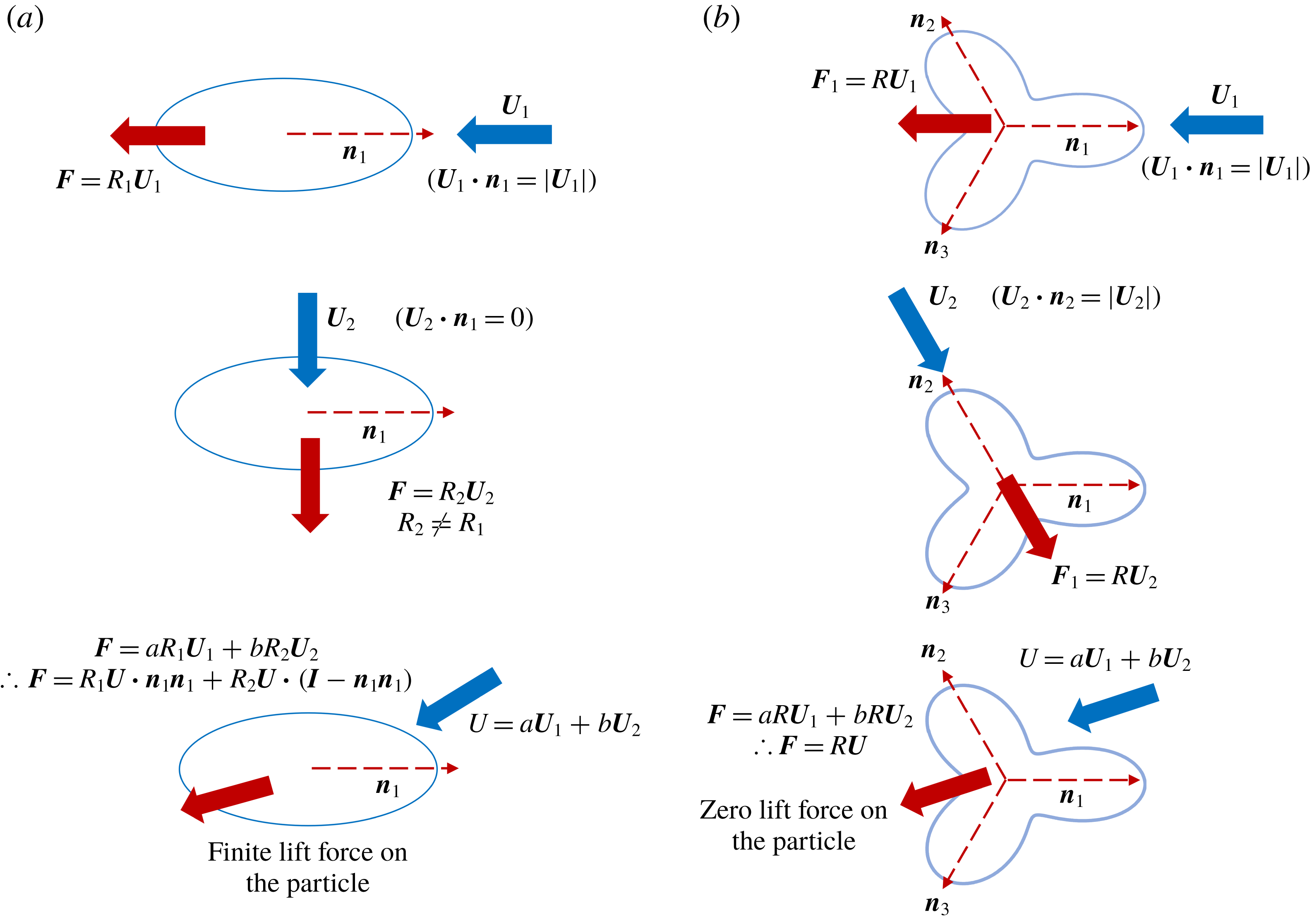
Thought experiments are presented using two-dimensional Stokes flow problems to gain physical insight into why only the second and third Fourier mode perturbations to a circle change the force per unit length acting on a long cylinder. Consider a two-dimensional obstacle, whose shape is a second Fourier mode perturbation to a circle, that is placed in a uniform flow field. This body experiences a lift force, unless the imposed fluid velocity is along one of its two axes of symmetries as shown in figure 2(a). The third and higher Fourier mode perturbations to a circle have at least a twofold rotational symmetry in a two-dimensional space. An
 $N$
-fold rotational symmetry means that the shape looks the same after rotating it by any integer multiple of
 $2\unicode[STIX]{x03C0}/N$
. These cross-sections cannot generate a lift force in a two-dimensional (2-D) uniform flow along at least two non-colinear directions,
 $\boldsymbol{n}_{\mathbf{1}}$
and
 $\boldsymbol{n}_{\mathbf{2}}$
as shown in figure 2(b), due to fore–aft symmetry. Thereby such a cross-section should experience no lift for all cross-sectional orientations by linear superposition. This is analogous to our result obtained earlier that only slender particles with cross-sections with a second Fourier mode perturbation to a circle will experience an additional force per unit length.
Schematic of thought experiments to intuitively understand the importance of the second Fourier mode perturbation to a circle. (a) Finite lift on a second Fourier mode perturbation of a circle. (b) Zero lift force on a cross-section with a three-lobed cross-section which is obtained from the third Fourier mode perturbation to a circle. This zero lift is true for the third and any higher Fourier mode perturbation to a circle.

To gain insight into the force per unit length driven by the gradient in the imposed fluid velocity, consider a cross-section placed in a general linear flow field and note that at
 $O(\unicode[STIX]{x1D6FC})$
the influence of the Fourier mode perturbations can be linearly superimposed. Only the extensional component of the flow influences the force per unit length,
 $\breve{\boldsymbol{f}}$
. Using the linearity of Stokes equations,
 $\breve{\boldsymbol{f}}$
is given by
 $$\begin{eqnarray}\breve{\boldsymbol{f}}=\unicode[STIX]{x1D709}_{1}\unicode[STIX]{x1D640}_{\boldsymbol{\infty }}\boldsymbol{ : }\boldsymbol{n}_{\boldsymbol{k}}\boldsymbol{n}_{\boldsymbol{k}}\boldsymbol{n}_{\boldsymbol{k}}+\unicode[STIX]{x1D709}_{2}\unicode[STIX]{x1D640}_{\boldsymbol{\infty }}\boldsymbol{\cdot }\boldsymbol{n}_{\boldsymbol{k}},\end{eqnarray}$$
where
 $\unicode[STIX]{x1D640}_{\boldsymbol{\infty }}$
is the straining tensor of the linear flow field and
 $\boldsymbol{n}_{\boldsymbol{k}}=[\cos (2\unicode[STIX]{x03C0}k/n),\sin (2\unicode[STIX]{x03C0}k/n)]$
with
 $k=0,1,\ldots ,(n-1)$
being the orientations along the lines of symmetry of the
 $n$
th Fourier mode perturbation to the circle (
 $n\geqslant 2$
). Choosing
 $\unicode[STIX]{x1D640}_{\infty }=\left[\!\begin{smallmatrix}0 & 1\\ 1 & 0\end{smallmatrix}\!\right]$
,
 $\breve{\boldsymbol{f}}$
can be written as
 $$\begin{eqnarray}\breve{\boldsymbol{f}}=\left[\begin{array}{@{}c@{}}\displaystyle \left(2\cos ^{2}\left(\frac{2\unicode[STIX]{x03C0}}{n}k\right)\unicode[STIX]{x1D709}_{1}+\unicode[STIX]{x1D709}_{2}\right)\sin \left(\frac{2\unicode[STIX]{x03C0}}{n}k\right)\\ \displaystyle \left(2\sin ^{2}\left(\frac{2\unicode[STIX]{x03C0}}{n}k\right)\unicode[STIX]{x1D709}_{1}+\unicode[STIX]{x1D709}_{2}\right)\cos \left(\frac{2\unicode[STIX]{x03C0}}{n}k\right)\end{array}\right]=\left[\begin{array}{@{}c@{}}0\\ \unicode[STIX]{x1D709}_{2}\end{array}\right]_{k=0},\end{eqnarray}$$
where the second equality gives the value
 $\breve{\boldsymbol{f}}$
at
 $k=0$
.
 $\breve{\boldsymbol{f}}$
as per (3.7b
) can be identical and non-zero for
 $\forall k\in \{0,1,\ldots ,(n-1)\}$
only for the third Fourier mode perturbation to a circle. Identical values of
 $\breve{\boldsymbol{f}}$
for any other Fourier mode perturbation would require
 $\unicode[STIX]{x1D709}_{1}=\unicode[STIX]{x1D709}_{2}=0$
implying
 $\breve{\boldsymbol{f}}=\mathbf{0}$
. This implies that at linear order in the perturbation parameter, the force per unit length is only affected by the third Fourier mode perturbation. One can get a visual picture for the existence of
 $\breve{\boldsymbol{f}}=[0~\unicode[STIX]{x1D709}_{2}]$
, using our linear perturbation analysis for
 $u_{\unicode[STIX]{x1D703}}^{\prime }$
. For
 $\unicode[STIX]{x1D640}_{\infty }=\left[\!\begin{smallmatrix}0 & 1\\ 1 & 0\end{smallmatrix}\!\right]$
, the perturbation to the tangential velocity
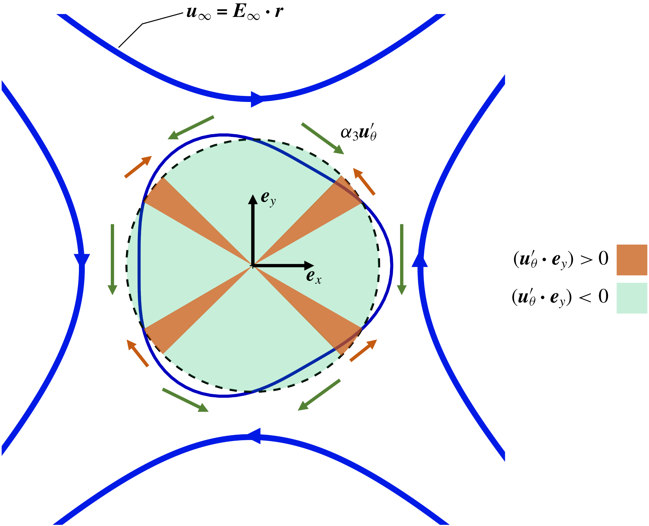
 $\unicode[STIX]{x1D6FC}_{3}u_{\unicode[STIX]{x1D703}}^{\prime }=-\unicode[STIX]{x1D6FC}_{3}(4\cos (2\unicode[STIX]{x1D703})\cos (3\unicode[STIX]{x1D703}))$
is required to satisfy the no-slip condition on the particle surface. The direction of
 $u_{\unicode[STIX]{x1D703}}^{\prime }$
shown in figure 3, suggests that
 $u_{\unicode[STIX]{x1D703}}^{\prime }$
points along
 $-\boldsymbol{e}_{\boldsymbol{y}}$
for
 $\unicode[STIX]{x1D703}\in \{(0,\unicode[STIX]{x03C0}/6),(\unicode[STIX]{x03C0}/4,3\unicode[STIX]{x03C0}/4),(5\unicode[STIX]{x03C0}/6,7\unicode[STIX]{x03C0}/6),(5\unicode[STIX]{x03C0}/4,7\unicode[STIX]{x03C0}/4),(11\unicode[STIX]{x03C0}/6,2\unicode[STIX]{x03C0})\}$
and points along
 $\boldsymbol{e}_{\boldsymbol{y}}$
for the remaining narrow portions of angular space. A net average velocity along
 $(-\boldsymbol{e}_{\boldsymbol{y}})$
is required to satisfy the no-slip boundary condition which leads to the force
 $\breve{\boldsymbol{f}}=(0,\unicode[STIX]{x1D709}_{2})$
along that direction.
Direction of the perturbation to the tangential velocity on the particle surface
 $\unicode[STIX]{x1D6FC}_{3}u_{\unicode[STIX]{x1D703}}^{\prime }=-\unicode[STIX]{x1D6FC}_{3}(4\cos (2\unicode[STIX]{x1D703})\cos (3\unicode[STIX]{x1D703}))$
necessary to satisfy the no-slip condition suggesting a need for a force along
 $\boldsymbol{e}_{\boldsymbol{y}}$
.

The additional terms in the longitudinal velocity field used during the matching process are given by
 $$\begin{eqnarray}\unicode[STIX]{x1D6FC}u_{z}^{\prime }=\unicode[STIX]{x1D6FC}e_{0}^{\prime }+\unicode[STIX]{x1D6FC}E^{\prime }\ln \left(\frac{\unicode[STIX]{x1D70C}}{a}\right)+\cdots ,\end{eqnarray}$$
where
 $e_{0}^{\prime }$
is obtained from the no-slip boundary condition and
 $E^{\prime }$
is determined by matching the inner solution to the outer solution in a similar manner to obtaining
 $E$
. Substituting
 $\unicode[STIX]{x1D70C}=a(1+\unicode[STIX]{x1D6FC}h)$
in (2.8), it can be shown that there is no term of
 $O(\unicode[STIX]{x1D6FC})$
which does not depend on
 $\unicode[STIX]{x1D703}$
, and therefore
 $e_{0}^{\prime }$
is zero.
The velocity field in the inner region for a cross-section given by
 $\unicode[STIX]{x1D70C}=a(1+\unicode[STIX]{x1D6FC}h)$
, which could be obtained from (2.4) to (2.6), (3.2), (3.3) and (3.8), is given by
 $$\begin{eqnarray}u_{i}^{\mathit{inner}}=u_{i}+\unicode[STIX]{x1D6FC}u_{i}^{\prime },\end{eqnarray}$$
where
 $i=\{\unicode[STIX]{x1D70C},\unicode[STIX]{x1D703},z\}$
.
3.2 Matching the inner and outer velocity field for a slightly non-circular cross-section
Due to the linearity of Stokes equations, the additional force per unit length that arises from the perturbation of the circular cross-section must be of the form (
 $\unicode[STIX]{x1D6FC}\boldsymbol{f}^{\prime }$
), where
 $|\,\boldsymbol{f}^{\prime }|$
is at most
 $O(\unicode[STIX]{x1D716}^{2})$
. The outer velocity disturbance created by
 $\boldsymbol{f}^{\prime }$
should also have a form similar to the velocity disturbance created by
 $\boldsymbol{f}$
, i.e.
 $$\begin{eqnarray}\displaystyle \boldsymbol{u}^{\prime }(\boldsymbol{r}) & {\approx} & \displaystyle -\frac{1}{4\unicode[STIX]{x03C0}}(\boldsymbol{I}+\boldsymbol{e}_{\boldsymbol{z}}\boldsymbol{e}_{\boldsymbol{z}})\boldsymbol{\cdot }\boldsymbol{f}^{\prime }(\boldsymbol{r})\left[\ln \left(\frac{\unicode[STIX]{x1D70C}}{2}\right)-\ln \left(\frac{s(1-s)}{a(s)}\right)\right]-\frac{1}{4\unicode[STIX]{x03C0}}\boldsymbol{f}^{\prime }\boldsymbol{\cdot }\boldsymbol{e}_{\boldsymbol{ z}}\boldsymbol{e}_{\boldsymbol{z}}+\frac{1}{4\unicode[STIX]{x03C0}}\boldsymbol{f}^{\prime }\boldsymbol{\cdot }\boldsymbol{e}_{\unicode[STIX]{x1D70C}}\boldsymbol{e}_{\unicode[STIX]{x1D70C}}\nonumber\\ \displaystyle & & \displaystyle +\,\frac{1}{8\unicode[STIX]{x03C0}}\int _{\boldsymbol{r}_{\boldsymbol{c}}}\,\text{d}s^{\prime }\left[\left(\frac{\boldsymbol{I}}{|\boldsymbol{r}_{\boldsymbol{c}}(s)-\boldsymbol{r}_{\boldsymbol{c}}(s^{\prime })|}+\frac{(\boldsymbol{r}_{\boldsymbol{c}}(s)-\boldsymbol{r}_{\boldsymbol{c}}(s^{\prime }))(\boldsymbol{r}_{\boldsymbol{ c}}(s)-\boldsymbol{r}_{\boldsymbol{c}}(s^{\prime }))}{|\boldsymbol{r}_{\boldsymbol{c}}(s)-\boldsymbol{r}_{\boldsymbol{c}}(s^{\prime })|^{3}}\right)\right.\nonumber\\ \displaystyle & & \displaystyle \boldsymbol{\cdot }\left.\boldsymbol{f}^{\prime }(\boldsymbol{r}^{\prime })-\left(\frac{\boldsymbol{I}}{|s-s^{\prime }|}+\frac{\boldsymbol{e}_{\boldsymbol{z}}\boldsymbol{e}_{\boldsymbol{z}}}{|s-s^{\prime }|}\right)\boldsymbol{\cdot }\boldsymbol{f}^{\prime }(\boldsymbol{r})\right].\end{eqnarray}$$
The complete velocity field,
 $\boldsymbol{u}+\unicode[STIX]{x1D6FC}\boldsymbol{u}^{\prime }$
, is obtained by combining (2.8) and (3.10). On matching the velocity fields from the inner and outer region,
 $\boldsymbol{f}^{\prime }$
is given by the integral equation
 $$\begin{eqnarray}\displaystyle \boldsymbol{f}^{\prime }(\boldsymbol{r}) & = & \displaystyle \frac{\unicode[STIX]{x1D716}}{2}\left(\boldsymbol{I}-\frac{\boldsymbol{e}_{\boldsymbol{z}}\boldsymbol{e}_{\boldsymbol{z}}}{2}\right)\boldsymbol{\cdot }\left(\frac{C^{\prime }}{2}\boldsymbol{e}_{\boldsymbol{y}}-\frac{D^{\prime }}{2}\boldsymbol{e}_{\boldsymbol{x}}-\frac{1}{8\unicode[STIX]{x03C0}}(\boldsymbol{I}-3\boldsymbol{e}_{\boldsymbol{z}}\boldsymbol{e}_{\boldsymbol{z}})\boldsymbol{\cdot }\boldsymbol{f}^{\prime }(\boldsymbol{r})\right.\nonumber\\ \displaystyle & & \displaystyle -\,\frac{1}{4\unicode[STIX]{x03C0}}(\boldsymbol{I}+\boldsymbol{e}_{\boldsymbol{z}}\boldsymbol{e}_{\boldsymbol{z}})\boldsymbol{\cdot }\boldsymbol{f}^{\prime }(\boldsymbol{r})\ln \left(\frac{s(1-s)}{a(s)}\right)\nonumber\\ \displaystyle & & \displaystyle +\,\frac{1}{8\unicode[STIX]{x03C0}}\int _{\boldsymbol{r}_{\boldsymbol{c}}}\,\text{d}s^{\prime }\left[\left(\frac{\boldsymbol{I}}{|\boldsymbol{r}_{\boldsymbol{c}}(s)-\boldsymbol{r}_{\boldsymbol{c}}(s^{\prime })|}+\frac{(\boldsymbol{r}_{\boldsymbol{c}}(s)-\boldsymbol{r}_{\boldsymbol{c}}(s^{\prime }))(\boldsymbol{r}_{\boldsymbol{ c}}(s)-\boldsymbol{r}_{\boldsymbol{c}}(s^{\prime }))}{|\boldsymbol{r}_{\boldsymbol{c}}(s)-\boldsymbol{r}_{\boldsymbol{c}}(s^{\prime })|^{3}}\right)\right.\nonumber\\ \displaystyle & & \displaystyle \boldsymbol{\cdot }\left.\left.\boldsymbol{f}^{\prime }(\boldsymbol{r}^{\prime })-\left(\frac{\boldsymbol{I}}{|s-s^{\prime }|}+\frac{\boldsymbol{e}_{\boldsymbol{z}}\boldsymbol{e}_{\boldsymbol{z}}}{|s-s^{\prime }|}\right)\boldsymbol{\cdot }\boldsymbol{f}^{\prime }(\boldsymbol{r})\right]\right).\end{eqnarray}$$
Here,
 $\boldsymbol{f}^{\prime }$
can be iteratively obtained with errors of
 $O(\unicode[STIX]{x1D716}^{N+1})$
or errors of
 $O(\unicode[STIX]{x1D716}^{N}/A)$
if
 $h_{2}=0$
, where
 $N\geqslant 2$
;
 $\boldsymbol{f}^{\prime }$
does not have a component along the longitudinal direction at linear order in
 $\unicode[STIX]{x1D6FC}$
. This can be understood on matching the
 $O(\unicode[STIX]{x1D6FC})$
terms in the inner and outer velocity fields in
 $u_{z}^{\prime }$
, which results in
 $E^{\prime }$
being identically zero.
The integral equation for the net force per unit length,
 $\boldsymbol{f}_{\boldsymbol{n}\boldsymbol{e}\boldsymbol{t}}=\boldsymbol{f}+\unicode[STIX]{x1D6FC}\boldsymbol{f}^{\prime }$
is given by
 $$\begin{eqnarray}\displaystyle \frac{(\,\boldsymbol{f}_{net})}{8\unicode[STIX]{x03C0}} & = & \displaystyle \frac{\unicode[STIX]{x1D716}}{2}\left(\boldsymbol{I}-\frac{\boldsymbol{e}_{\boldsymbol{z}}\boldsymbol{e}_{\boldsymbol{z}}}{2}\right)\boldsymbol{\cdot }\left\{\boldsymbol{U}+\unicode[STIX]{x1D74E}\times \boldsymbol{r}_{\boldsymbol{c}}-\boldsymbol{u}_{\boldsymbol{\infty }}(\boldsymbol{r}_{\boldsymbol{c}})+\unicode[STIX]{x1D6FC}\left(\frac{C^{\prime }}{2}\boldsymbol{e}_{\boldsymbol{y}}-\frac{D^{\prime }}{2}\boldsymbol{e}_{\boldsymbol{x}}\right)\right.\nonumber\\ \displaystyle & & \displaystyle -\,\frac{1}{8\unicode[STIX]{x03C0}}(\boldsymbol{I}-3\boldsymbol{e}_{\boldsymbol{z}}\boldsymbol{e}_{\boldsymbol{z}})\boldsymbol{\cdot }(\,\boldsymbol{f}_{\boldsymbol{n}\boldsymbol{e}\boldsymbol{t}})-\frac{1}{4\unicode[STIX]{x03C0}}(\boldsymbol{I}+\boldsymbol{e}_{\boldsymbol{z}}\boldsymbol{e}_{\boldsymbol{z}})\boldsymbol{\cdot }(\,\boldsymbol{f}_{\boldsymbol{n}\boldsymbol{e}\boldsymbol{t}})\ln \left(\frac{s(1-s)}{a(s)}\right)\nonumber\\ \displaystyle & & \displaystyle +\,\frac{1}{8\unicode[STIX]{x03C0}}\int _{\boldsymbol{r}_{\boldsymbol{c}}}\,\text{d}s^{\prime }\left[\left(\frac{\boldsymbol{I}}{|\boldsymbol{r}_{\boldsymbol{c}}(s)-\boldsymbol{r}_{\boldsymbol{c}}(s^{\prime })|}+\frac{(\boldsymbol{r}_{\boldsymbol{c}}(s)-\boldsymbol{r}_{\boldsymbol{c}}(s^{\prime }))(\boldsymbol{r}_{\boldsymbol{ c}}(s)-\boldsymbol{r}_{\boldsymbol{c}}(s^{\prime }))}{|\boldsymbol{r}_{\boldsymbol{c}}(s)-\boldsymbol{r}_{\boldsymbol{c}}(s^{\prime })|^{3}}\right)\right.\nonumber\\ \displaystyle & & \displaystyle \boldsymbol{\cdot }\left.\!\left.(\,\boldsymbol{f}_{\boldsymbol{n}\boldsymbol{e}\boldsymbol{t}}(\boldsymbol{r}^{\prime }))-\left(\frac{\boldsymbol{I}}{|s-s^{\prime }|}+\frac{\boldsymbol{e}_{\boldsymbol{z}}\boldsymbol{e}_{\boldsymbol{z}}}{|s-s^{\prime }|}\right)\boldsymbol{\cdot }(\,\boldsymbol{f}_{\boldsymbol{n}\boldsymbol{e}\boldsymbol{t}}(\boldsymbol{r}))\right]\right\},\end{eqnarray}$$
where
 $C^{\prime }$
and
 $D^{\prime }$
are obtained from (3.2) and (3.3), respectively, and have contributions of order
 $\unicode[STIX]{x1D716}$
and/or
 $1/A$
depending on the shape of the cross-section. The governing integral equation can be completely solved to get the value of the force per unit length correct to
 $O(\unicode[STIX]{x1D716}^{N})+O(\unicode[STIX]{x1D6FC}\unicode[STIX]{x1D716}^{N+1})+O(\unicode[STIX]{x1D6FC}\unicode[STIX]{x1D716}^{N}/\text{A})$
, where
 $N$
is an integer greater that unity. Solving for the force per unit length to
 $O(\unicode[STIX]{x1D716})+O(\unicode[STIX]{x1D6FC}\unicode[STIX]{x1D716}^{2})+O(\unicode[STIX]{x1D6FC}\unicode[STIX]{x1D716}/A)$
, equation (3.12) simplifies to
 $$\begin{eqnarray}\boldsymbol{f}+\unicode[STIX]{x1D6FC}\boldsymbol{f}^{\prime }=4\unicode[STIX]{x03C0}\unicode[STIX]{x1D716}(\boldsymbol{U}+\unicode[STIX]{x1D74E}\times \boldsymbol{r}_{\boldsymbol{ c}}-\boldsymbol{u}_{\boldsymbol{\infty }}(\boldsymbol{r}_{\boldsymbol{c}}))\boldsymbol{\cdot }\left(\boldsymbol{I}-\frac{\boldsymbol{e}_{\boldsymbol{z}}\boldsymbol{e}_{\boldsymbol{z}}}{2}\right)+2\unicode[STIX]{x03C0}\unicode[STIX]{x1D716}\unicode[STIX]{x1D6FC}(-D^{\prime }\boldsymbol{e}_{\boldsymbol{ x}}+C^{\prime }\boldsymbol{e}_{\boldsymbol{ y}}).\end{eqnarray}$$
Equation (3.13) suggests that the force per unit length experienced by a slender filament due to non-circularity of the cross-section is affected at
 $O(\unicode[STIX]{x1D6FC}\unicode[STIX]{x1D716}^{2})$
due to the velocity disturbance of the unperturbed circular cross-section and at
 $O(\unicode[STIX]{x1D6FC}\unicode[STIX]{x1D716}/A)$
due to the gradient in the imposed fluid velocity.
3.3 Extending the analysis to a general cross-sectional shape
$(\unicode[STIX]{x1D6FC}\sim O(1))$

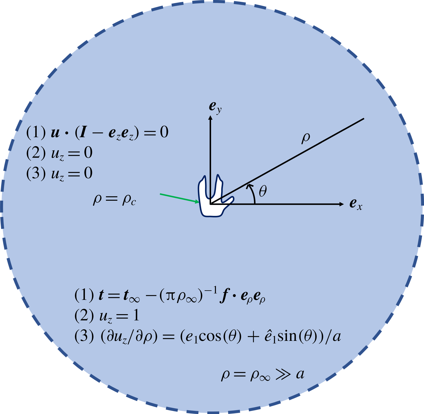
Here, a numerical calculation to determine the velocity disturbance by any cross-section is elucidated which can be used as the matching solution for SBT. This calculation involves the solution to the flow past an obstacle with the same shape as the particle cross-section in a two-dimensional domain with a size,
 $\unicode[STIX]{x1D70C}_{\infty }$
, that is much larger than the cross-sectional size (
 $\unicode[STIX]{x1D70C}_{\infty }\gg a$
) as shown in figure 4. In this subsection, the fluid viscosity, a measure of the undisturbed fluid velocity far away from the obstacle and a length that is of the order of the size of the obstacle are used to non-dimensionalize any quantity of interest, such as the force per unit length.
Schematic of the two-dimensional domain to obtain
 $\unicode[STIX]{x1D646}$
and
 $\boldsymbol{L}$
, along with the boundary conditions for (1) the 2-D Stokes flow equations in the transverse plane and the Laplace equation for the longitudinal velocity field
 $\unicode[STIX]{x1D6FB}^{2}u_{z}=0$
for computing (2)
 $\unicode[STIX]{x1D612}_{zz}$
and (3)
 $L_{z}$
.

The apparent hydrodynamic centre of resistance (AHCOR) of the cross-section is chosen as the centre of the computational domain to avoid a solid body rotation at large separations from the particle. The AHCOR is defined as the point about which zero torque is acting on a two-dimensional obstacle translating in a concentric circular domain of size much larger than the obstacle with the outer boundary having zero velocity. (AHCOR is similar to the hydrodynamic centre of resistance for three-dimensional particles, which is defined as the point about which the torque acting on a body translating in a quiescent fluid is zero (Kim & Karrila Reference Kim and Karrila1991). In a two-dimensional Stokes flow the velocity disturbance due to an obstacle grows logarithmically with the domain size and therefore a hydrodynamic centre of resistance based on the above definition cannot be defined in the same manner.)
Consider a stationary obstacle experiencing a force per unit length
 $\boldsymbol{f}$
placed in a fluid with an imposed velocity of
 $\boldsymbol{u}_{\boldsymbol{\infty }}\boldsymbol{\cdot }(\boldsymbol{I}-\boldsymbol{e}_{\boldsymbol{z}}\boldsymbol{e}_{\boldsymbol{z}})$
. The velocity field at the outer boundary is obtained from the asymptotic form predicted by SBT according to (2.8) and (3.11). This asymptotic form of the imposed fluid velocity in the region
 $\unicode[STIX]{x1D70C}\gg a$
is given by
 $$\begin{eqnarray}\boldsymbol{u}=\boldsymbol{u}_{\boldsymbol{\infty }}+\frac{2\boldsymbol{f}}{8\unicode[STIX]{x03C0}}\boldsymbol{\cdot }\left[-\ln \left(\frac{\unicode[STIX]{x1D70C}}{a}\right)(\boldsymbol{I}+\boldsymbol{e}_{\boldsymbol{z}}\boldsymbol{e}_{\boldsymbol{z}})+(\boldsymbol{e}_{\unicode[STIX]{x1D746}}\boldsymbol{e}_{\unicode[STIX]{x1D746}}-0.5(\boldsymbol{I}-\boldsymbol{e}_{\boldsymbol{z}}\boldsymbol{e}_{\boldsymbol{z}}))+\unicode[STIX]{x1D646}\right]+\boldsymbol{L},\end{eqnarray}$$
where
 $\unicode[STIX]{x1D646}$
is a second-order tensor that depends only on the geometry of the particle cross-section and
 $\boldsymbol{L}$
is a vector that arises due to the gradient of the imposed fluid velocity and therefore depends both on the geometry of the particle and
 $\boldsymbol{u}_{\infty }$
. The tensor
 $\unicode[STIX]{x1D646}$
is symmetric (Batchelor Reference Batchelor1970), such that
 $\unicode[STIX]{x1D612}_{iz}=\unicode[STIX]{x1D612}_{zi}=0$
for
 $i=\{x,y\}$
, due to the decoupling of the longitudinal and the transverse flow fields around a long slender body. The corresponding pressure for this velocity field in the region
 $\unicode[STIX]{x1D70C}\gg a$
is given by
 $$\begin{eqnarray}p=\frac{4}{8\unicode[STIX]{x03C0}\unicode[STIX]{x1D70C}}\boldsymbol{f}\boldsymbol{\cdot }\boldsymbol{e}_{\unicode[STIX]{x1D746}}.\end{eqnarray}$$
In (3.14),
 $\unicode[STIX]{x1D646}$
and
 $\boldsymbol{L}$
are to be determined as part of the solution and therefore the velocity field at the outer boundary for a given
 $\boldsymbol{f}$
and
 $\boldsymbol{u}_{\boldsymbol{\infty }}$
cannot be specified a priori. Instead, the force per unit area
 $\boldsymbol{t}$
acting on the outer boundary
 $\unicode[STIX]{x1D70C}=\unicode[STIX]{x1D70C}_{\infty }$
is specified. Here
 $\boldsymbol{t}$
is independent of
 $a$
,
 $\unicode[STIX]{x1D646}$
and
 $\boldsymbol{L}$
, and given by
 $$\begin{eqnarray}\boldsymbol{t}=\boldsymbol{t}_{\boldsymbol{\infty }}-\frac{1}{\unicode[STIX]{x03C0}\unicode[STIX]{x1D70C}_{\infty }}\boldsymbol{f}\boldsymbol{\cdot }(\boldsymbol{e}_{\unicode[STIX]{x1D746}}\boldsymbol{e}_{\unicode[STIX]{x1D746}}),\end{eqnarray}$$
where
 $\boldsymbol{t}_{\boldsymbol{\infty }}$
is the force per unit area that would act on the outer boundary due to
 $\boldsymbol{u}_{\boldsymbol{\infty }}\boldsymbol{\cdot }(\boldsymbol{I}-\boldsymbol{e}_{\boldsymbol{z}}\boldsymbol{e}_{\boldsymbol{z}})$
in the absence of the obstacle.
The values of
 $a$
and
 $\unicode[STIX]{x1D612}_{ij}$
for
 $i,j=\{x,y\}$
are obtained by solving the 2-D Stokes equations with no slip on the obstacle surface and
 $\boldsymbol{t}=-(1/\unicode[STIX]{x03C0}\unicode[STIX]{x1D70C}_{\infty })\boldsymbol{f}\boldsymbol{\cdot }(\boldsymbol{e}_{\unicode[STIX]{x1D746}}\boldsymbol{e}_{\unicode[STIX]{x1D746}})$
on the outer boundary and matching the numerical velocity field to
 $\boldsymbol{u}\boldsymbol{\cdot }(\boldsymbol{I}-\boldsymbol{e}_{\boldsymbol{z}}\boldsymbol{e}_{\boldsymbol{z}})$
with
 $\boldsymbol{L}=0$
at the outer boundary. Also,
 $L_{i}$
for
 $i=\{1,2\}$
is calculated by equating
 $\boldsymbol{u}=(\boldsymbol{u}_{\boldsymbol{\infty }}+\boldsymbol{L})\boldsymbol{\cdot }(\boldsymbol{I}-\boldsymbol{e}_{\boldsymbol{z}}\boldsymbol{e}_{\boldsymbol{z}})$
to the velocity field at the outer boundary obtained from the solution of the 2-D Stokes equations with no slip on the obstacle surface and
 $\boldsymbol{t}=\boldsymbol{t}_{\boldsymbol{\infty }}$
at
 $\unicode[STIX]{x1D70C}=\unicode[STIX]{x1D70C}_{\infty }$
. Further,
 $u_{z}$
at the outer boundary obtained from the solution of
 $\unicode[STIX]{x1D6FB}^{2}u_{z}=0$
, with no-slip on the obstacle and a constant value at
 $\unicode[STIX]{x1D70C}=\unicode[STIX]{x1D70C}_{\infty }$
, is equated to
 $u_{z}$
from (3.14) to obtain
 $\unicode[STIX]{x1D612}_{zz}$
. Similarly,
 $u_{z}$
at the outer boundary obtained from the solution of
 $\unicode[STIX]{x1D6FB}^{2}u_{z}=0$
, with no slip on the obstacle and
 $\unicode[STIX]{x2202}u_{z}/\unicode[STIX]{x2202}\unicode[STIX]{x1D70C}$
corresponding to a linear vector field
 $\boldsymbol{u}_{\boldsymbol{\infty }}\boldsymbol{\cdot }\boldsymbol{e}_{\boldsymbol{z}}$
at
 $\unicode[STIX]{x1D70C}=\unicode[STIX]{x1D70C}_{\infty }$
, is equated to
 $u_{z}$
from (3.14) to obtain
 $L_{z}$
. For arbitrary cross-sections the 2-D Stokes flow equations and the 2-D Laplace’s equation can be solved using a finite element solver such as COMSOL or a two-dimensional boundary element method, by choosing a
 $\unicode[STIX]{x1D70C}_{\infty }$
which is sufficiently large such that the values of
 $a$
,
 $\unicode[STIX]{x1D646}$
and
 $\boldsymbol{L}$
do not change on further increasing
 $\unicode[STIX]{x1D70C}_{\infty }$
. The final integral equation for the force per unit length exerted by a slender filament with an arbitrary cross-section is given by
 $$\begin{eqnarray}\displaystyle \frac{\boldsymbol{f}(\boldsymbol{r})}{8\unicode[STIX]{x03C0}} & = & \displaystyle \frac{\unicode[STIX]{x1D716}}{2}\left(\boldsymbol{I}-\frac{\boldsymbol{e}_{\boldsymbol{z}}\boldsymbol{e}_{\boldsymbol{z}}}{2}\right)\boldsymbol{\cdot }\left\{\boldsymbol{U}+\unicode[STIX]{x1D74E}\times \boldsymbol{r}_{\boldsymbol{c}}-\boldsymbol{u}_{\boldsymbol{\infty }}(\boldsymbol{r}_{\boldsymbol{c}})+\frac{1}{4\unicode[STIX]{x03C0}}\boldsymbol{f}(\boldsymbol{r})\boldsymbol{\cdot }\unicode[STIX]{x1D646}+\boldsymbol{L}\right.\nonumber\\ \displaystyle & & \displaystyle -\,\frac{1}{8\unicode[STIX]{x03C0}}(\boldsymbol{I}-3\boldsymbol{e}_{\boldsymbol{z}}\boldsymbol{e}_{\boldsymbol{z}})\boldsymbol{\cdot }\boldsymbol{f}(\boldsymbol{r})-\frac{1}{4\unicode[STIX]{x03C0}}(\boldsymbol{I}+\boldsymbol{e}_{\boldsymbol{z}}\boldsymbol{e}_{\boldsymbol{z}})\boldsymbol{\cdot }\boldsymbol{f}(\boldsymbol{r})\ln \left(\frac{s(1-s)}{a(s)}\right)\nonumber\\ \displaystyle & & \displaystyle +\,\frac{1}{8\unicode[STIX]{x03C0}}\int _{\boldsymbol{r}_{\boldsymbol{c}}}\,\text{d}s^{\prime }\left[\left(\frac{\boldsymbol{I}}{|\boldsymbol{r}_{\boldsymbol{c}}(s)-\boldsymbol{r}_{\boldsymbol{c}}(s^{\prime })|}+\frac{(\boldsymbol{r}_{\boldsymbol{c}}(s)-\boldsymbol{r}_{\boldsymbol{c}}(s^{\prime }))(\boldsymbol{r}_{\boldsymbol{ c}}(s)-\boldsymbol{r}_{\boldsymbol{c}}(s^{\prime }))}{|\boldsymbol{r}_{\boldsymbol{c}}(s)-\boldsymbol{r}_{\boldsymbol{c}}(s^{\prime })|^{3}}\right)\right.\nonumber\\ \displaystyle & & \displaystyle \boldsymbol{\cdot }\left.\!\left.\boldsymbol{f}(\boldsymbol{r}^{\prime })-\left(\frac{\boldsymbol{I}}{|s-s^{\prime }|}+\frac{\boldsymbol{e}_{\boldsymbol{z}}\boldsymbol{e}_{\boldsymbol{z}}}{|s-s^{\prime }|}\right)\boldsymbol{\cdot }\boldsymbol{f}(\boldsymbol{r})\right]\right\}.\end{eqnarray}$$
Note that
 $\unicode[STIX]{x1D646}$
is related to the tensor
 $\unicode[STIX]{x1D646}_{\boldsymbol{B}}$
and
 $\ln (k_{B})$
, which Batchelor (Reference Batchelor1970) mentions in (5.5) and (6.1) of his paper respectively, by the relation
 $\unicode[STIX]{x1D646}_{\boldsymbol{B}}+2\ln (k_{B})\boldsymbol{e}_{\boldsymbol{z}}\boldsymbol{e}_{\boldsymbol{z}}=\unicode[STIX]{x1D646}+(\boldsymbol{I}+\boldsymbol{e}_{\boldsymbol{z}}\boldsymbol{e}_{\boldsymbol{z}})\ln (a/R_{B})$
, where
 $R_{B}$
is such that
 $2\unicode[STIX]{x03C0}R_{B}$
is the perimeter of the cross-section. Batchelor (Reference Batchelor1970) shows that
 $\unicode[STIX]{x1D646}_{\boldsymbol{B}}$
is a symmetric tensor, which implies that
 $\unicode[STIX]{x1D646}$
is also symmetric. The tensor
 $\unicode[STIX]{x1D646}_{\boldsymbol{B}}$
has three unknowns such that
 $\unicode[STIX]{x1D646}_{\boldsymbol{B}}\boldsymbol{\cdot }\boldsymbol{e}_{\boldsymbol{z}}=\mathbf{0}$
. These unknowns are written in terms of
 $a$
and
 $\unicode[STIX]{x1D612}_{ij}$
, where
 $i,j=\{x,y\}$
, such that
 $\unicode[STIX]{x1D612}_{xx}+\unicode[STIX]{x1D612}_{yy}=0$
. Also,
 $\unicode[STIX]{x1D612}_{zz}=2\ln (k_{B})-2\ln (a/R_{B})$
captures the effect of the cross-sectional shape on the force and velocity field in the longitudinal direction. The influence of the cross-section on the velocity disturbance in the transverse plane can be decomposed into an isotropic component
 $\ln (a)\boldsymbol{I}$
and a traceless component
 $\unicode[STIX]{x1D646}-\unicode[STIX]{x1D612}_{zz}\boldsymbol{e}_{\boldsymbol{z}}\boldsymbol{e}_{\boldsymbol{z}}$
. This length scale ‘
 $a$
’ which arises as part of the hydrodynamic calculation is therefore used instead of a purely geometric length scale
 $R_{B}$
.
The second order tensor
 $\unicode[STIX]{x1D646}$
can be represented in terms of
 $\overline{\unicode[STIX]{x1D6FC}}_{2}$
,
 $\unicode[STIX]{x1D703}_{02}$
and
 $\unicode[STIX]{x1D612}_{zz}$
and is given by
 $$\begin{eqnarray}\unicode[STIX]{x1D646}=\left[\begin{array}{@{}ccc@{}}-0.5\overline{\unicode[STIX]{x1D6FC}}_{2}\cos (2\unicode[STIX]{x1D703}_{02}) & -0.5\overline{\unicode[STIX]{x1D6FC}}_{2}\sin (2\unicode[STIX]{x1D703}_{02}) & 0\\ -0.5\overline{\unicode[STIX]{x1D6FC}}_{2}\sin (2\unicode[STIX]{x1D703}_{02}) & 0.5\overline{\unicode[STIX]{x1D6FC}}_{2}\cos (2\unicode[STIX]{x1D703}_{02}) & 0\\ 0 & 0 & \unicode[STIX]{x1D612}_{zz}\end{array}\right].\end{eqnarray}$$
 $(\overline{\unicode[STIX]{x1D6FC}}_{2},\unicode[STIX]{x1D703}_{02})$
, similar to
 $(\unicode[STIX]{x1D6FC}_{2},\unicode[STIX]{x1D703}_{02})$
of the regular perturbation theory, give the contribution to the second Fourier mode of the cross-sectional geometry.
 $\unicode[STIX]{x1D612}_{zz}$
, which is zero to leading order in the perturbation analysis, can have a non-zero value for a general cross-sectional shape. This is because
 $u_{z}$
can be affected by the details of the cross-section at
 $O(\unicode[STIX]{x1D6FC}^{2})$
(see supplementary material S.2 for details). The vector
 $\boldsymbol{L}$
can represented in terms of
 $\overline{\unicode[STIX]{x1D6FC}}_{3}$
,
 $\unicode[STIX]{x1D703}_{03}$
,
 $L_{z}$
and the imposed fluid velocity and is given by
 $$\begin{eqnarray}\boldsymbol{L}=\left[\begin{array}{@{}c@{}}2\overline{\unicode[STIX]{x1D6FC}}_{3}(\hat{a}_{2}\cos (3\unicode[STIX]{x1D703}_{03})-a_{2}\sin (3\unicode[STIX]{x1D703}_{03}))\\ 2\overline{\unicode[STIX]{x1D6FC}}_{3}(a_{2}\cos (3\unicode[STIX]{x1D703}_{03})+\hat{a}_{2}\sin (3\unicode[STIX]{x1D703}_{03}))\\ L_{zx}e_{1}+L_{zy}\hat{e}_{1}\end{array}\right],\end{eqnarray}$$
where the imposed velocity field
 $(\boldsymbol{u}_{\boldsymbol{\infty }}(\boldsymbol{r})-\boldsymbol{u}_{\boldsymbol{\infty }}(\boldsymbol{r}_{\boldsymbol{c}}))\boldsymbol{\cdot }(\boldsymbol{I}-\boldsymbol{e}_{\boldsymbol{z}}\boldsymbol{e}_{\boldsymbol{z}})$
is specified in terms of a streamfunction
 $\unicode[STIX]{x1D713}_{\infty }$
given by
 $$\begin{eqnarray}\frac{\unicode[STIX]{x1D713}_{\infty }}{a}=\tilde{a}_{0}\left(\frac{\unicode[STIX]{x1D70C}}{a}\right)^{2}+(a_{2}\cos (2\unicode[STIX]{x1D703})+\hat{a}_{2}\sin (2\unicode[STIX]{x1D703}))\left(\frac{\unicode[STIX]{x1D70C}}{a}\right)^{2},\end{eqnarray}$$
and
 $(\boldsymbol{u}_{\boldsymbol{\infty }}(\boldsymbol{r})-\boldsymbol{u}_{\boldsymbol{\infty }}(\boldsymbol{r}_{\boldsymbol{c}}))\boldsymbol{\cdot }\boldsymbol{e}_{\boldsymbol{z}}\boldsymbol{e}_{\boldsymbol{z}}$
is given by
 $$\begin{eqnarray}u_{\infty ,z}=(e_{1}\cos (\unicode[STIX]{x1D703})+\hat{e}_{1}\sin (\unicode[STIX]{x1D703}))\frac{\unicode[STIX]{x1D70C}}{a},\end{eqnarray}$$
 $(\overline{\unicode[STIX]{x1D6FC}}_{3},\unicode[STIX]{x1D703}_{03})$
, similar to
 $(\unicode[STIX]{x1D6FC}_{3},\unicode[STIX]{x1D703}_{03})$
of the regular perturbation theory, give the contribution to the third Fourier mode perturbation. The longitudinal component
 $\boldsymbol{L}\boldsymbol{\cdot }\boldsymbol{e}_{\boldsymbol{z}}$
is zero in the linear perturbation analysis but it is non-zero for a general cross-sectional geometry. The longitudinal component of
 $-\boldsymbol{L}$
is the longitudinal velocity at which a particle must translate to avoid a longitudinal force per unit length when it is subjected to a simple shear flow with the stagnation streamline coinciding with the AHCOR. For the geometries studied in this paper,
 $\boldsymbol{L}\boldsymbol{\cdot }\boldsymbol{e}_{\boldsymbol{z}}$
was found to be numerically small compared to the components of
 $\boldsymbol{L}$
in the transverse plane.
4 Resistance to motion of a triaxial ellipsoid
In this section our theory is utilized to obtain the Stokes hydrodynamic resistance tensor of triaxial ellipsoids of semi-axis lengths
 $l_{1}$
,
 $l_{2}$
and
 $l_{3}$
, such that
 $l_{3}\gg l_{1}>l_{2}$
(3 is the longitudinal direction, 1 is along the long axis of the elliptical cross-section and directions,
 $[1,2,3]$
form a right-handed Cartesian coordinate system). By symmetry of the shape, the force,
 $\boldsymbol{F}$
and the torque,
 $\boldsymbol{T}$
acting on the ellipsoid are given as
 $\boldsymbol{F}=\unicode[STIX]{x1D64D}^{\boldsymbol{F}\boldsymbol{U}}\boldsymbol{\cdot }\boldsymbol{U}$
,
 $\boldsymbol{T}=\unicode[STIX]{x1D64D}^{\boldsymbol{L}\unicode[STIX]{x1D74E}}\boldsymbol{\cdot }\unicode[STIX]{x1D74E}$
, where
 $\unicode[STIX]{x1D64D}^{\boldsymbol{F}\boldsymbol{U}}$
and
 $\unicode[STIX]{x1D64D}^{\boldsymbol{L}\unicode[STIX]{x1D74E}}$
are
 $3\times 3$
diagonal matrices that depend only on the particle geometry. The values of
 $\unicode[STIX]{x1D64D}^{\boldsymbol{F}\boldsymbol{U}}$
and
 $\unicode[STIX]{x1D64D}^{\boldsymbol{L}\unicode[STIX]{x1D74E}}$
for
 $l_{3}/l_{1}\gg 1$
and
 $(l_{1}-l_{2})/l_{1}\ll 1$
using the perturbation analysis in § 3.2 are given by
 $$\begin{eqnarray}\displaystyle & \displaystyle \unicode[STIX]{x1D64D}^{\boldsymbol{F}\boldsymbol{U}}=(8\unicode[STIX]{x03C0}){\displaystyle \frac{\unicode[STIX]{x1D716}(2l_{3})}{2+\unicode[STIX]{x1D716}}}\left[\begin{array}{@{}ccc@{}}1-{\displaystyle \frac{\unicode[STIX]{x1D6FC}_{2}\unicode[STIX]{x1D716}}{2+\unicode[STIX]{x1D716}}} & 0 & 0\\ 0 & 1+{\displaystyle \frac{\unicode[STIX]{x1D6FC}_{2}\unicode[STIX]{x1D716}}{2+\unicode[STIX]{x1D716}}} & 0\\ 0 & 0 & {\displaystyle \frac{1}{2}}{\displaystyle \frac{2+\unicode[STIX]{x1D716}}{2-\unicode[STIX]{x1D716}}}\end{array}\right], & \displaystyle\end{eqnarray}$$
 $$\begin{eqnarray}\displaystyle & \displaystyle \unicode[STIX]{x1D64D}^{\boldsymbol{L}\unicode[STIX]{x1D74E}}=(8\unicode[STIX]{x03C0})\frac{2l_{3}^{3}}{3}\frac{\unicode[STIX]{x1D716}}{2-\unicode[STIX]{x1D716}}\left[\begin{array}{@{}ccc@{}}1+{\displaystyle \frac{\unicode[STIX]{x1D6FC}_{2}\unicode[STIX]{x1D716}}{2-\unicode[STIX]{x1D716}}} & 0 & 0\\ 0 & 1-{\displaystyle \frac{\unicode[STIX]{x1D6FC}_{2}\unicode[STIX]{x1D716}}{2-\unicode[STIX]{x1D716}}} & 0\\ 0 & 0 & {\displaystyle \frac{(2-\unicode[STIX]{x1D716})}{\unicode[STIX]{x1D716}}}\left({\displaystyle \frac{a}{l_{3}}}\right)^{2}\end{array}\right], & \displaystyle\end{eqnarray}$$
where
 $\unicode[STIX]{x1D716}=1/\ln (2l_{3}/a)$
.
 $a$
and
 $\unicode[STIX]{x1D6FC}_{2}$
are given by
 $a=0.5(l_{1}+l_{2})$
and
 $\unicode[STIX]{x1D6FC}_{2}=(l_{1}-l_{2})/(2a)$
for
 $(l_{1}-l_{2})\ll l_{1}$
. The results of (4.1) and (4.2) match exactly with the values obtained by Batchelor (Reference Batchelor1970) (equations (8.7), (8.8) and (8.10) of his paper).
For cross-sections with
 $(l_{1}-l_{2})\sim O(l_{1})$
,
 $\unicode[STIX]{x1D64D}^{\boldsymbol{F}\boldsymbol{U}}$
and
 $\unicode[STIX]{x1D64D}^{\boldsymbol{L}\unicode[STIX]{x1D74E}}$
are determined using the numerical procedure in § 3.3 and the results retain great accuracy even for cross-sections with extreme aspect ratio. COMSOL, a finite element solver, was used to perform the 2-D Stokes flow calculation. The second order tensor
 $\unicode[STIX]{x1D646}$
was estimated with an uncertainty of below 0.1 % when the size of the outer boundary (
 $\unicode[STIX]{x1D70C}_{\infty }$
) was at least 30 times the cross-sectional dimension. Figure 5 shows the deviation of
 $\unicode[STIX]{x1D64D}^{\boldsymbol{F}\boldsymbol{U}}$
and
 $\unicode[STIX]{x1D64D}^{\boldsymbol{L}\unicode[STIX]{x1D74E}}$
predicted by our numerical procedure from the exact result for an ellipsoid given by Lamb (Reference Lamb1932) for a high aspect ratio elliptical cross-section with
 $l_{1}/l_{2}=10$
. The deviation of the SBT for a circular cross-section from the exact result is also presented for comparison. Our SBT predicts
 $\unicode[STIX]{x1D64D}^{\boldsymbol{F}\boldsymbol{U}}$
and
 $\unicode[STIX]{x1D64D}^{\boldsymbol{L}\unicode[STIX]{x1D74E}}$
better than the SBT results for a circular cross-section and has errors less than approximately 1 % for
 $l_{3}/l_{1}\gtrsim 10$
. The high level of accuracy shows the applicability of our methodology to accurately predict the resistance to motion of slender bodies with arbitrary cross-section.
The value of
 $\unicode[STIX]{x1D64D}^{\boldsymbol{L}\unicode[STIX]{x1D74E}}\boldsymbol{ : }\boldsymbol{e}_{\mathbf{3}}\boldsymbol{e}_{\mathbf{3}}$
needs special attention for a straight slender body because the force per unit length cannot generate a torque about its longitudinal axis. To obtain the effect of the cross-sectional geometry on
 $\unicode[STIX]{x1D64D}^{\boldsymbol{L}\unicode[STIX]{x1D74E}}\boldsymbol{ : }\boldsymbol{e}_{\mathbf{3}}\boldsymbol{e}_{\mathbf{3}}$
, a two-dimensional Stokes flow problem is solved to find the torque per unit length
 $\boldsymbol{g}\propto a^{2}(s)$
acting on an ellipse with sides
 $l_{1}$
and
 $l_{2}$
which is rotating with a unit angular velocity parallel to
 $\boldsymbol{e}_{\mathbf{3}}$
with the velocity on the outer boundary set to zero (see figure 3). The torque per unit length is integrated by accounting for the variation of the cross-sectional size to attain the total torque on the ellipsoid, and thereby obtain
 $\unicode[STIX]{x1D64D}^{\boldsymbol{L}\unicode[STIX]{x1D74E}}\boldsymbol{ : }\boldsymbol{e}_{\mathbf{3}}\boldsymbol{e}_{\mathbf{3}}$
as depicted in figure 5(f).
Variation of resistances,
 $\unicode[STIX]{x1D64D}^{\boldsymbol{F}\boldsymbol{U}}$
and
 $\unicode[STIX]{x1D64D}^{\boldsymbol{L}\unicode[STIX]{x1D74E}}$
, with
 $l_{3}/l_{1}$
for an ellipsoid with
 $l_{1}/l_{2}=10$
. (a–f) Comparison of
 $\unicode[STIX]{x0394}\unicode[STIX]{x1D619}_{ij}^{k}=(\unicode[STIX]{x1D619}_{ij}^{k}-(\unicode[STIX]{x1D619}_{ij}^{k})_{\mathit{exact}})/(\unicode[STIX]{x1D619}_{ij}^{k})_{\mathit{exact}}$
, the deviation of different components of
 $\unicode[STIX]{x1D64D}^{\boldsymbol{F}\boldsymbol{U}}$
and
 $\unicode[STIX]{x1D64D}^{\boldsymbol{L}\unicode[STIX]{x1D74E}}$
predicted using the current SBT as well as the SBT for a circular cross-section from the exact result of Lamb (Reference Lamb1932) (
 $(\unicode[STIX]{x1D619}_{ij}^{k})_{\mathit{exact}}$
). Here
 $i,j=\{1,2,3\}$
and
 $k=\{\boldsymbol{F}\boldsymbol{U},\boldsymbol{L}\unicode[STIX]{x1D74E}\}$
.

5 Translation of a straight slender body in a simple shear flow (SSF)
An axisymmetric straight particle rotates periodically in one of the Jeffery orbits depending on its initial orientation and has zero cross-stream drift relative to the fluid velocity at its centre of mass. A straight particle with a three-lobed cross-section shown in figure 6(a) rotates like a spheroid but translates quasi-periodically across streamlines with an
 $O(\unicode[STIX]{x1D6FC}/A)$
velocity. A straight particle with a combination of an elliptic (or two-lobed) and a three-lobed cross-section can rotate chaotically and translate diffusively. The calculations in this section can be used to extract the motion of straight fibres in viscous fluids which is important in the manufacturing process of fibre-reinforced composite materials or paper products. The half-length of the particle, the shear rate and the fluid viscosity are used to non-dimensionalize variables in this section.
Schematic of the particle shape and the coordinate system used in the calculation. (a) Schematic of the slender particle that is longitudinally rectangular or elliptic. The cross-section of the particle is given by
 $\unicode[STIX]{x1D70C}_{s}=a(1+\unicode[STIX]{x1D6FC}_{3}\cos (3\unicode[STIX]{x1D703}))$
, where
 $\unicode[STIX]{x1D703}$
is measured from
 $\boldsymbol{n}$
. Here,
 $\boldsymbol{n}$
is along one of the lines of symmetry of the cross-section,
 $\hat{\boldsymbol{Y}}$
is a unit vector in the cross-sectional plane chosen such that
 $\hat{\boldsymbol{Y}}\boldsymbol{\cdot }\hat{\boldsymbol{U}}_{\boldsymbol{\infty }}=0$
and
 $\hat{\boldsymbol{X}}=\hat{\boldsymbol{Y}}\times \boldsymbol{p}$
. (b) The fixed reference frame is defined along the flow (
 $\hat{\boldsymbol{U}}_{\boldsymbol{\infty }}$
), vorticity (
 $\hat{\unicode[STIX]{x1D734}}_{\boldsymbol{\infty }}$
) and the gradient (
 $\hat{\unicode[STIX]{x1D71E}}_{\boldsymbol{\infty }}$
) direction of the SSF. The longitudinal direction of the particle is along
 $\boldsymbol{p}$
and a reference vector in the transverse plane is
 $\boldsymbol{n}$
;
 $\boldsymbol{p}$
,
 $\hat{\unicode[STIX]{x1D734}}_{\boldsymbol{\infty }}$
,
 $\unicode[STIX]{x1D646}=\boldsymbol{p}\times \hat{\unicode[STIX]{x1D734}}_{\boldsymbol{\infty }}$
,
 $\boldsymbol{n}$
and
 $\hat{\boldsymbol{U}}_{\infty }$
are used to define the Euler angles
 $\unicode[STIX]{x1D703}_{J},\unicode[STIX]{x1D719}_{J},\unicode[STIX]{x1D713}_{J}$
.

5.1 Problem formulation and SBT solution
The cross-section of the slender particle studied here is a small perturbation to a circle given by
 $\unicode[STIX]{x1D70C}_{s}=a(1+\unicode[STIX]{x1D6FC}_{3}\cos (3\unicode[STIX]{x1D703}))$
, where
 $\unicode[STIX]{x1D6FC}_{3}\ll 1$
is the perturbation parameter and
 $\unicode[STIX]{x1D703}$
is measured relative to a vector
 $\boldsymbol{n}$
that is along one of the lines of symmetry of the cross-section. The second Fourier mode perturbation to a circle does not affect
 $C^{\prime }$
and
 $D^{\prime }$
for a torque-free particle in a SSF because the force per unit length it produces satisfies
 $\boldsymbol{f}\boldsymbol{\cdot }(\boldsymbol{I}-\boldsymbol{p}\boldsymbol{p})=0$
. The second Fourier mode perturbation to a circle affects the torque per unit length
 $\boldsymbol{g}$
thereby influencing the rotational dynamics of a straight particle, which is discussed in § 5.3.
The size of the cross-section, ‘
 $a$
’, either varies with the longitudinal position,
 $s$
, as
 $a(s)/a_{0}=(1-s^{2})^{0.5}$
for a cross-section that is longitudinally elliptic or is a constant
 $a=a_{0}$
for a cylinder. The force per unit length obtained from (3.17), is used to obtain the linear (
 $\boldsymbol{U}$
) and angular (
 $\unicode[STIX]{x1D74E}$
) velocity of the particle by applying the force-free (
 $\int \boldsymbol{f}_{net}\,\text{d}s=0$
) and torque-free (
 $\int (s\boldsymbol{p}\times \boldsymbol{f}_{net}+\boldsymbol{g})\,\text{d}s=0$
) condition on the particle respectively. Here,
 $\boldsymbol{g}$
is calculated by computing the stresses from a transverse velocity field obtained from the stream function
 $\tilde{\unicode[STIX]{x1D713}}$
and the velocity field
 $\tilde{u} _{z}$
.
The angular velocity
 $\unicode[STIX]{x1D74E}$
is not affected by a three-lobed perturbation of a circle at linear order in
 $\unicode[STIX]{x1D6FC}_{3}$
and thus, this particle rotates periodically, like a spheroid shown by Jeffery (Reference Jeffery1922). This holds true for cylinders with blunt ends and a three-lobed cross-section. The ends of a blunt cylinder significantly influence
 $\unicode[STIX]{x1D74E}$
when the particle is near the flow–vorticity plane (Cox Reference Cox1971), which can be computed using the force generated at the ends of the particle in the transverse direction,
 $\boldsymbol{F}_{\boldsymbol{e}\boldsymbol{n}\boldsymbol{d}}$
. Using linearity of Stokes flow, and the symmetry of the third and higher Fourier mode perturbations,
 $\boldsymbol{g}\boldsymbol{\cdot }(\boldsymbol{I}-\boldsymbol{p}\boldsymbol{p})$
and
 $\boldsymbol{p}\times \boldsymbol{F}_{\boldsymbol{e}\boldsymbol{n}\boldsymbol{d}}$
can be shown to be proportional to
 $\unicode[STIX]{x1D640}\boldsymbol{\cdot }\boldsymbol{p}\times \boldsymbol{p}$
which is proportional to
 $\unicode[STIX]{x1D74E}$
due to the straining component of a SSF for an axisymmetric particle (see supplementary material S2). Therefore, straight particles with
 $\unicode[STIX]{x1D6FC}_{2}=0$
, in addition to circular cylinders shown by Cox (Reference Cox1971), rotate similar to an
 $O(A/\sqrt{\ln (A)})$
aspect ratio spheroid. The exact relationship can be obtained from experiments or a numerical calculation. For a torque-free straight particle with a three-lobed cross-section,
 $\unicode[STIX]{x1D74E}$
is given by
 $$\begin{eqnarray}\unicode[STIX]{x1D74E}=\unicode[STIX]{x1D74E}_{\boldsymbol{\infty }}+\unicode[STIX]{x1D706}_{J}\boldsymbol{p}\times (\unicode[STIX]{x1D640}\boldsymbol{\cdot }\boldsymbol{p}),\end{eqnarray}$$
where
 $\unicode[STIX]{x1D706}_{J}$
is the rotation parameter of the particle that depends only on its geometry. The rotation parameter
 $\unicode[STIX]{x1D706}_{J}=1-2/A^{2}$
for a slender particle that is longitudinally elliptic (Jeffery Reference Jeffery1922; Cox Reference Cox1971) and
 $\unicode[STIX]{x1D706}_{J}=1-0.65(\ln (A)/A^{2})$
for a cylinder, where the prefactor of 0.65 was obtained by fitting the asymptotic form of Cox (Reference Cox1971) to the experimental data of Anczurowski & Mason (Reference Anczurowski and Mason1968).
Unlike a spheroid or a circular cylinder, a slender particle with a three-lobed cross-section drifts across streamlines due to the
 $O(\unicode[STIX]{x1D6FC}_{3}/A)$
force per unit length. The drift velocity of the particle is confined to the plane normal to
 $\boldsymbol{p}$
, as
 $\boldsymbol{f}_{\boldsymbol{n}\boldsymbol{e}\boldsymbol{t}}\boldsymbol{\cdot }\boldsymbol{p}=0$
. Thus, the drift velocity of this particle takes the form
 $\boldsymbol{U}_{\boldsymbol{p}}=U_{x}\hat{\boldsymbol{X}}+U_{y}\hat{\boldsymbol{Y}}$
, where
 $U_{x}$
and
 $U_{y}$
are the components of the drift velocity along
 $\hat{\boldsymbol{X}}$
and
 $\hat{\boldsymbol{Y}}$
respectively and (
 $\hat{\boldsymbol{X}},\hat{\boldsymbol{Y}},\boldsymbol{p}$
) form an orthogonal pair such that
 $\hat{\boldsymbol{Y}}\boldsymbol{\cdot }\hat{\boldsymbol{U}}_{\boldsymbol{\infty }}=0$
.
 $U_{x}$
and
 $U_{y}$
are given by
 $$\begin{eqnarray}\displaystyle & U_{x}=\unicode[STIX]{x1D6FC}_{3}a_{0}U_{0}[\unicode[STIX]{x1D640}_{\boldsymbol{\infty }}\boldsymbol{ : }\hat{\boldsymbol{X}}\hat{\boldsymbol{Y}}\sin (3\unicode[STIX]{x1D703}_{0X})-0.5\unicode[STIX]{x1D640}_{\boldsymbol{\infty }}\boldsymbol{ : }\hat{\boldsymbol{X}}\hat{\boldsymbol{X}}\cos (3\unicode[STIX]{x1D703}_{0X})], & \displaystyle\end{eqnarray}$$
 $$\begin{eqnarray}\displaystyle & U_{y}=\unicode[STIX]{x1D6FC}_{3}a_{0}U_{0}[\unicode[STIX]{x1D640}_{\boldsymbol{\infty }}\boldsymbol{ : }\hat{\boldsymbol{X}}\hat{\boldsymbol{Y}}\cos (3\unicode[STIX]{x1D703}_{0X})+0.5\unicode[STIX]{x1D640}_{\boldsymbol{\infty }}\boldsymbol{ : }\hat{\boldsymbol{X}}\hat{\boldsymbol{X}}\sin (3\unicode[STIX]{x1D703}_{0X})], & \displaystyle\end{eqnarray}$$
 $U_{0}=1$
for a cylinder and
 $U_{0}=\unicode[STIX]{x03C0}/4$
for a spheroid,
 $\unicode[STIX]{x1D703}_{0X}$
is the angle made by
 $\hat{\boldsymbol{X}}$
with
 $\boldsymbol{n}$
and
 $\unicode[STIX]{x1D640}_{\boldsymbol{\infty }}={\textstyle \frac{1}{2}}(\unicode[STIX]{x1D735}\boldsymbol{u}^{\boldsymbol{\infty }}+(\unicode[STIX]{x1D735}\boldsymbol{u}^{\boldsymbol{\infty }})^{\text{T}})$
is the straining tensor. Here,
 $\boldsymbol{U}$
for the longitudinally elliptic particle differs from
 $\boldsymbol{U}$
of a cylinder by a factor of
 $\unicode[STIX]{x03C0}/4$
due to the difference in the integral of
 $\int _{-1}^{1}\text{d}s~a(s)$
for the two cases. Only the results for a straight cylinder are presented in the following section, since both
 $\boldsymbol{U}$
and
 $\unicode[STIX]{x1D74E}$
are qualitatively similar for a longitudinally elliptic particle.
5.2 Quasi-periodic translation of particles
The motion of the particle shown in figure 6(a) is calculated by tracking its centre of mass position and orientation. The orientation is given in terms of the Euler angles, (
 $\unicode[STIX]{x1D703}_{J},\unicode[STIX]{x1D713}_{J},\unicode[STIX]{x1D719}_{J}$
), shown in figure 6(b) and defined using the longitudinal direction of the particle
 $\boldsymbol{p}=(\sin (\unicode[STIX]{x1D719}_{J})\sin (\unicode[STIX]{x1D703}_{J}),\cos (\unicode[STIX]{x1D703}_{J}),\cos (\unicode[STIX]{x1D719}_{J})\sin (\unicode[STIX]{x1D703}_{J}))$
, a vector
 $\boldsymbol{K}=(\cos (\unicode[STIX]{x1D719}_{J}),0,-\sin (\unicode[STIX]{x1D719}_{J}))$
that is normal to both
 $\boldsymbol{p}$
and
 $\hat{\unicode[STIX]{x1D734}}_{\boldsymbol{\infty }}$
and
 $\cos (\unicode[STIX]{x1D713}_{J})=\boldsymbol{n}\boldsymbol{\cdot }\boldsymbol{K}$
, where
 $\boldsymbol{n}$
is a vector along one of the lines of symmetry of the cross-section as illustrated in figure 6(a). Here,
 $(\boldsymbol{n},\boldsymbol{b},\boldsymbol{p})$
and
 $(\hat{\boldsymbol{X}},\hat{\boldsymbol{Y}},\boldsymbol{p})$
, such that
 $\hat{\boldsymbol{Y}}\boldsymbol{\cdot }\hat{\boldsymbol{U}}_{\boldsymbol{\infty }}=0$
, form an orthogonal set. The angle
 $\unicode[STIX]{x1D703}_{0X}$
in (5.4) equals
 $\text{asin}(\hat{\boldsymbol{Y}}\boldsymbol{\cdot }\boldsymbol{n})$
. Jeffery (Reference Jeffery1922) obtained the time variation of
 $\unicode[STIX]{x1D719}_{J}$
and
 $\unicode[STIX]{x1D703}_{J}$
that is given by
 $$\begin{eqnarray}\displaystyle & \displaystyle \tan (\unicode[STIX]{x1D719}_{J})=A_{e}\tan \left(2\unicode[STIX]{x03C0}\frac{t}{T}+\unicode[STIX]{x1D70F}\right), & \displaystyle\end{eqnarray}$$
 $$\begin{eqnarray}\displaystyle & \displaystyle \tan (\unicode[STIX]{x1D703}_{J})=\frac{A_{e}C}{\sqrt{A_{e}^{2}\cos ^{2}(\unicode[STIX]{x1D719}_{J})+\sin ^{2}(\unicode[STIX]{x1D719}_{J})}}, & \displaystyle\end{eqnarray}$$
where
 $\unicode[STIX]{x1D719}_{J}\in [0,2\unicode[STIX]{x03C0})$
,
 $\unicode[STIX]{x1D703}_{J}\in [0,\unicode[STIX]{x03C0}]$
,
 $C$
is the orbit constant,
 $\unicode[STIX]{x1D70F}$
is the phase angle,
 $T=2\unicode[STIX]{x03C0}(A_{e}+A_{e}^{-1})$
is the period of rotation of
 $\boldsymbol{p}$
and
 $A_{e}$
is the effective aspect ratio of the particle defined as
 $A_{e}=\sqrt{(1+\unicode[STIX]{x1D706}_{J})/(1-\unicode[STIX]{x1D706}_{J})}$
. A thin cylinder (
 $A\gg 1$
) spends most of its time such that
 $\boldsymbol{p}$
is near the flow–vorticity plane (
 $\unicode[STIX]{x1D719}_{J}\rightarrow \unicode[STIX]{x03C0}/2$
). The rate of change of
 $\unicode[STIX]{x1D713}_{J}$
is given by
 $$\begin{eqnarray}\frac{\text{d}\unicode[STIX]{x1D713}_{J}}{\text{d}t}=-\frac{1}{2}\unicode[STIX]{x1D706}_{J}\cos (\unicode[STIX]{x1D703}_{J})\cos (2\unicode[STIX]{x1D719}_{J}).\end{eqnarray}$$
According to (5.3c
),
 $\unicode[STIX]{x1D713}_{J}$
changes over a time scale of
 $O((1+(A_{e}C)^{2})^{0.5})$
which varies with the orbit constant,
 $C$
, and contrasts from the fixed
 $O(T)$
time scale over which
 $\unicode[STIX]{x1D703}_{J}$
and
 $\unicode[STIX]{x1D719}_{J}$
change. Therefore, there are uncountably infinite orbits where
 $\unicode[STIX]{x1D713}_{J}$
rotates quasi-periodically while only countably infinite orbits where
 $\unicode[STIX]{x1D713}_{J}$
has a period that is a multiple of
 $T$
. The quasi-periodic rotation of
 $\unicode[STIX]{x1D713}_{J}$
demonstrates that the
 $(\unicode[STIX]{x1D713}_{J},\unicode[STIX]{x1D719}_{J})$
space is filled completely over time as seen in figure 7(b,c). Discrete peaks in the frequency spectrum obtained by the fast Fourier transformation
 $\hat{\unicode[STIX]{x1D713}}_{J}$
is used to establish the quasi-periodic nature of the system as shown in figure 7(d).
Trajectory of the orientation of the particle. (a) Orientational trajectory of
 $\boldsymbol{p}$
(
 $\unicode[STIX]{x1D706}_{J}=0.98$
) for various initial conditions specified by the orbit constant,
 $C$
. Change in (
 $\unicode[STIX]{x1D713},\unicode[STIX]{x1D719}$
) during (b) 10 and (c)
 $10^{3}$
tumbling events respectively for a cylinder with
 $A=20$
and
 $C=0.1$
. (d) Frequency spectrum obtained from the fast Fourier transformation of
 $\unicode[STIX]{x1D713}_{J}(t)$
for
 $C=0.1$
and
 $A=20$
.

The average velocity of the particle is zero because of the symmetry of the orbits relative to the SSF. The quasiperiodic translation is quantified using the root mean square (r.m.s.) velocity of the particle given by
 $$\begin{eqnarray}\langle (\boldsymbol{U}\boldsymbol{\cdot }\unicode[STIX]{x1D73B})^{2}\rangle ^{1/2}=\lim _{N\rightarrow \infty }\frac{1}{\sqrt{NT}}\left(\sqrt{\int _{0}^{NT}(\boldsymbol{U}\boldsymbol{\cdot }\unicode[STIX]{x1D73B})^{2}\,\text{d}t}\right),\end{eqnarray}$$
where
 $\unicode[STIX]{x1D73B}\in \{\hat{\unicode[STIX]{x1D734}}_{\boldsymbol{\infty }},\hat{\unicode[STIX]{x1D71E}}_{\boldsymbol{\infty }}\}$
and
 $N$
should be sufficiently large such that the results are invariant on increasing
 $N$
. The mean-square velocity can also be obtained by averaging in the
 $(\unicode[STIX]{x1D713}_{J},\unicode[STIX]{x1D719}_{J})$
space given by
 $$\begin{eqnarray}\langle (\boldsymbol{U}\boldsymbol{\cdot }\unicode[STIX]{x1D73B})^{2}\rangle =\int _{0}^{2\unicode[STIX]{x03C0}}\text{d}\unicode[STIX]{x1D719}_{J}\left(\frac{1}{2\unicode[STIX]{x03C0}}\right)\left(\frac{A_{e}(1-\unicode[STIX]{x1D706})}{1+\unicode[STIX]{x1D706}\cos (2\unicode[STIX]{x1D719}_{J})}\right)\int _{0}^{2\unicode[STIX]{x03C0}}\text{d}\unicode[STIX]{x1D713}_{J}\frac{1}{2\unicode[STIX]{x03C0}}(\boldsymbol{U}\boldsymbol{\cdot }\unicode[STIX]{x1D73B})^{2}.\end{eqnarray}$$
The r.m.s. velocity in the gradient (
 $\hat{\unicode[STIX]{x1D71E}}_{\boldsymbol{\infty }}$
) and vorticity (
 $\hat{\unicode[STIX]{x1D734}}_{\boldsymbol{\infty }}$
) direction for
 $\unicode[STIX]{x1D6FC}_{3}=0.1$
are shown in figures 8(a) and 8(b), respectively, as a function of
 $C$
for varying particle aspect ratios. The r.m.s. velocities computed from (5.5) match the values obtained from time averaging over 500 tumbling events reaffirming the quasi-periodic nature of the system. For
 $C\rightarrow 0$
the particle is symmetric about the flow–gradient plane and therefore cannot translate in the vorticity direction as evident in figure 8(b). In this orbit
 $\hat{\boldsymbol{X}}=\hat{\boldsymbol{U}}_{\boldsymbol{\infty }}$
and
 $\hat{\boldsymbol{Y}}=\hat{\unicode[STIX]{x1D71E}}_{\boldsymbol{\infty }}$
thereby leading to the highest value of
 $U_{y}$
among the orbits as per (5.2). Therefore,
 $\langle (\boldsymbol{U}\boldsymbol{\cdot }\hat{\unicode[STIX]{x1D71E}}_{\boldsymbol{\infty }})^{2}\rangle$
is highest when
 $C=0$
and monotonically decreases with increasing
 $C$
as seen in figure 8(a). A peak is observed in
 $\langle (\boldsymbol{U}\boldsymbol{\cdot }\hat{\unicode[STIX]{x1D734}}_{\boldsymbol{\infty }})^{2}\rangle$
for
 $C\sim O(1/A)$
before the value plateaus for large
 $C\gg 1$
.
Particle r.m.s. velocity variation with particle aspect ratio,
 $A$
, and orbit constant,
 $C$
for
 $\unicode[STIX]{x1D6FC}_{3}=0.1$
. Root mean square velocity of the particle in (a) the gradient direction and (b) the vorticity direction averaged over 500 tumbling events. Solid lines are phase-space integration using (5.5), while the symbols are the results of the time integration (5.4).

These qualitatively new results predicting cross-stream drift due to cross-sectional asymmetries can be compared to the drift velocities observed for curved fibres (Wang et al.
Reference Wang, Tozzi, Graham and Klingenberg2012) and screw-like particles (Kim & Rae Reference Kim and Rae1991). Curved fibres with an aspect ratio 20 and a curvature of unity migrate in the gradient direction with an average velocity of
 $1.7\times 10^{-3}$
(Wang et al.
Reference Wang, Tozzi, Graham and Klingenberg2012). The drift velocity of screw shaped particles is shown to be
 $O(10^{-4})$
, where the length and time are non-dimensionalized using the length of the screw along its axis and the inverse of the shear rate, respectively. (The diameter of the screw was 1, the diameter of the filament was 0.1, and the screw had two turns.) Both these values which are numerically comparable to the values in figure 8(a) suggest that the translation of slender bodies caused by cross-sectional modifications can have a similar magnitude to the effects of the shape of the centreline.
5.3 Diffusive translation of particles
Chaotic rotation and diffusive translation of a straight particle with a cross-section that is a combination of an ellipse and a third Fourier mode perturbation to a circle is demonstrated. The cross-section is given by
 $\unicode[STIX]{x1D70C}_{s}=(l_{1}^{2}\cos ^{2}(\unicode[STIX]{x1D703}-\unicode[STIX]{x1D703}_{02})+l_{2}^{2}\sin ^{2}(\unicode[STIX]{x1D703}-\unicode[STIX]{x1D703}_{02}))^{0.5}+a\unicode[STIX]{x1D6FC}_{3}\cos (3\unicode[STIX]{x1D703})$
, where
 $l_{1}$
,
 $l_{2}$
are lengths of the semi-major axes of an ellipse such that
 $l_{1}>l_{2}$
,
 $a$
is the radius of the equivalent circle of the ellipse with semi-axes
 $l_{1}$
,
 $l_{2}$
obtained from the analysis in § 3.3 and
 $\unicode[STIX]{x1D6FC}_{3}$
is the amplitude of the third Fourier mode perturbation to the equivalent circle. The cross-section is chosen to be longitudinally elliptic (i.e.
 $a/a_{0}=l_{1}/l_{1,0}=l_{2}/l_{2,0}=(1-s^{2})^{0.5}$
) with
 $\unicode[STIX]{x1D703}_{02}=0$
as such particles are known to rotate chaotically when
 $\unicode[STIX]{x1D6FC}_{3}=0$
(Yarin et al.
Reference Yarin, Gottlieb and Roisman1997). The rotational motion of such particles can be described using Jeffery’s (Reference Jeffery1922) equations of motion since the third Fourier mode perturbation does not alter
 $\unicode[STIX]{x1D74E}$
as shown earlier. Yarin et al. (Reference Yarin, Gottlieb and Roisman1997) demonstrated chaotic rotation of a particle with
 $\unicode[STIX]{x1D6FC}_{3}=0$
,
 $l_{1,0}=2/10$
and
 $l_{2,0}=1/10$
(an ellipsoid). Such a particle with a finite
 $\unicode[STIX]{x1D6FC}_{3}=0.2$
would translate diffusively in addition to rotating chaotically. This particle has
 $a_{0}=1.5/10$
,
 $\unicode[STIX]{x1D646}$
is represented in terms of
 $\overline{\unicode[STIX]{x1D6FC}}_{2}=0.33$
,
 $\unicode[STIX]{x1D703}_{02}$
and
 $\unicode[STIX]{x1D612}_{zz}=0$
;
 $\boldsymbol{L}$
is represented in terms of
 $\overline{\unicode[STIX]{x1D6FC}}_{3}=0.20$
,
 $\unicode[STIX]{x1D703}_{03}=0$
and
 $L_{z}=0$
, according to (3.18). The values
 $\overline{\unicode[STIX]{x1D6FC}}_{2}=0.33$
,
 $\overline{\unicode[STIX]{x1D6FC}}_{3}=\unicode[STIX]{x1D6FC}_{3}$
and
 $\unicode[STIX]{x1D703}_{03}=0$
are accurate within 7 % error for
 $\forall \unicode[STIX]{x1D6FC}_{3}\leqslant 0.2$
and arbitrary
 $\unicode[STIX]{x1D703}_{02}$
.
Shape and chaotic dynamics of particles. (a) Representative shape that can rotate and translate chaotically in a SSF. (b) Poincaré map sampled when
 $\unicode[STIX]{x1D719}_{J}$
is a multiple of
 $\unicode[STIX]{x03C0}$
for the shape in (a) with
 $\unicode[STIX]{x1D6FC}_{3}=0.1$
,
 $l_{1,0}=2/10$
and
 $l_{2,0}=1/10$
that shows the chaotic sea. The closed loops represent trajectories in which
 $(\unicode[STIX]{x1D719}_{J},\unicode[STIX]{x1D703}_{J},\unicode[STIX]{x1D713}_{J})$
change quasi-periodically. A detailed Poincaré map can be seen in figure 6(a) of Yarin et al. (Reference Yarin, Gottlieb and Roisman1997). (c) Variation of
 $\langle r_{3}(t)r_{3}(t)\rangle$
with the time, suggests a diffusive behaviour of the particle position. (d) A straight rod with an
 $L$
-shaped, which can rotate chaotically and migrate diffusively. (e) A straight rod with a
 $Y$
-shaped cross-section that can rotate periodically and translate quasi-periodically. These particles can be fabricated using photolithography (Foulds & Parameswaran Reference Foulds and Parameswaran2006) or 3-D printing (Raney & Lewis Reference Raney and Lewis2015).

The particle motion is obtained using the numerical procedure mentioned in Yarin et al. (Reference Yarin, Gottlieb and Roisman1997) for ellipsoids. The Poincaré map sampled when
 $\unicode[STIX]{x1D719}_{J}$
is a multiple of
 $\unicode[STIX]{x03C0}$
shows the chaotic sea as seen in figure 9(b). A particle whose orientation starts within the sea will span it after enough time. The simulation was carried out for a time of
 $10^{4}T$
, where
 $T$
is the time period of rotation of a spheroid of the same aspect ratio,
 $A=1/a_{0}$
. The diffusivity in the gradient (
 $D_{33}$
) and vorticity (
 $D_{22}$
) direction, obtained from the position of the particle, is given by
 $$\begin{eqnarray}D_{ij}=\frac{1}{2}\lim _{t\rightarrow \infty }\frac{\text{d}}{\text{d}t}\langle r_{i}(t)r_{j}(t)\rangle .\end{eqnarray}$$
The variation of
 $\langle r_{3}r_{3}\rangle$
with time shown in figure 9(c) suggests a ballistic motion at short times and a diffusive behaviour for long times with a diffusivity of
 $4\times 10^{-5}$
. The diffusivity in the vorticity direction
 $D_{22}=6\times 10^{-8}$
is of much smaller magnitude. The current case is particularly interesting as the particle is self-dispersive at zero Reynolds number without Brownian diffusion or inter-particle interactions. This gradient diffusivity is numerically comparable to the gradient diffusivity of a fibre of the same length and aspect ratio
 $A$
due to interparticle interactions when the dimensional particle number density
 $n^{\ast }{L^{\ast }}^{3}\approx 0.37$
, where
 $L^{\ast }$
is the dimensional length of the particle (Rahnama et al.
Reference Rahnama, Koch, Iso and Cohen1993; Lopez & Graham Reference Lopez and Graham2007). Similarly, the gradient diffusivity of curved fibres with aspect ratios of approximately 20 is
 $O(10^{-5})$
(Wang, Graham & Klingenberg Reference Wang, Graham and Klingenberg2014), again of a magnitude similar to the influence of the cross-section.
The orientational dynamics in this section, illustrated for straight cylinders which are longitudinally elliptic, can be extended to other straight bodies with tapered ends using results from a complimentary study of Cox (Reference Cox1971). Cox (Reference Cox1971) obtained the
 $O(1/(\ln (A)A^{2}))$
torque acting on a stationary body with tapered ends and a circular cross-section held stationary in the flow–vorticity plane of the simple shear flow. This torque can be matched with the torque required to rotate the particle in a quiescent fluid to obtain
 $\unicode[STIX]{x1D74E}$
. On applying a regular perturbation of the inner solution of Cox (Reference Cox1971) one can extend his result to a slightly non-circular cross-section. The details can be found in Cox (Reference Cox1971) which is discussed in § (S.3) of the supplementary material.
For a cylinder with blunt edges, which is a more practical case, the analysis of Cox (Reference Cox1971) breaks down because the ends of the cylinder generate an
 $O(1/A^{2})$
torque on the particle. The torque on a stationary cylinder with blunt ends is equal to
 $2\boldsymbol{p}\times \boldsymbol{F}_{end}$
, where
 $\boldsymbol{F}_{end}$
is the force acting on an end of the particle. For a general shaped cross-section, one can find a second-order tensor
 $\unicode[STIX]{x1D63C}$
, such that
 $\boldsymbol{F}_{end}=\unicode[STIX]{x1D63C}\boldsymbol{\cdot }\boldsymbol{g}$
.
 $\unicode[STIX]{x1D63C}$
can be derived by taking three random orientations and finding
 $\boldsymbol{F}_{end}$
from experiments or numerical solutions of the Stokes equations. The part of
 $\unicode[STIX]{x1D74E}\boldsymbol{\cdot }(\boldsymbol{I}-\boldsymbol{p}\boldsymbol{p})$
driven by the straining part of the SSF, can be obtained by equating
 $2\boldsymbol{p}\times \boldsymbol{F}_{end}$
to the torque required to rotate a particle in a quiescent fluid
 $8\unicode[STIX]{x03C0}\unicode[STIX]{x1D74E}\boldsymbol{\cdot }(\boldsymbol{I}-\boldsymbol{p}\boldsymbol{p})/(3\ln (A))$
. The longitudinal component of the angular velocity
 $\unicode[STIX]{x1D74E}\boldsymbol{\cdot }\boldsymbol{p}$
can be obtained by matching the torque due to
 $\boldsymbol{g}\boldsymbol{\cdot }\boldsymbol{p}$
to
 $4\unicode[STIX]{x03C0}\unicode[STIX]{x1D74E}\boldsymbol{\cdot }\boldsymbol{p}\boldsymbol{p}\int \text{d}s~a^{2}$
(Cox Reference Cox1971). This can allow us to model the rotational dynamics of straight particles with a general cross-section and blunt edges using the SBT formulation. This calculation of the orientation dynamics of straight particles is important in predicting the structure and rheology of fibre suspensions which could be useful in paper-manufacturing research.
A straight rod with an
 $L$
-shaped cross-section shown in figure 9(d) has a finite value of
 $\overline{\unicode[STIX]{x1D6FC}}_{2}$
and
 $\overline{\unicode[STIX]{x1D6FC}}_{3}$
and thereby rotates and translates chaotically (a non-zero
 $\overline{\unicode[STIX]{x1D6FC}}_{2}$
is similar to an equivalent elliptic cross-section). A straight rod with a
 $Y$
-shaped cross-section shown in figure 9(e) has a non-zero value of
 $\overline{\unicode[STIX]{x1D6FC}}_{3}$
while
 $\overline{\unicode[STIX]{x1D6FC}}_{2}=0$
and therefore rotates periodically and translates quasi-periodically. These rods could be fabricated via multi-step photolithography (Foulds & Parameswaran Reference Foulds and Parameswaran2006) or 3-D printing (Raney & Lewis Reference Raney and Lewis2015) opening a pathway to experimentally verify our results and observe interesting dynamics. Einarsson et al. (Reference Einarsson, Mihiretie, Laas, Ankardal, Angilella, Hanstorp and Mehlig2016) measured the rotational motion of non-axisymmetric particles formed by connecting multiple micro-rods, which can simulate particles with two- or three-lobed cross-sections. The results presented here demonstrate the nature of cross-sectional shapes that can be used to control the rotational and translational dynamics of straight particles in a SSF.
6 Motion of rings in a simple shear flow (SSF)
In this section, the SBT is used to predict the dynamics of rings with non-circular cross-sections and the results are verified using boundary element method (BEM) calculations. The influence of the cross-sectional geometry on the rotational and translational motion of rings is established using analytical expressions. Rings with cross-sections that have
 $\overline{\unicode[STIX]{x1D6FC}}_{2}\neq 0$
rotate and translate periodically with no net migration over time if the contribution to the third Fourier mode,
 $\overline{\unicode[STIX]{x1D6FC}}_{3}$
, is below a critical value that depends on the aspect ratio. On the other hand, rings with a
 $\overline{\unicode[STIX]{x1D6FC}}_{3}\neq 0$
can attain an equilibrium orientation and can drift indefinitely in the gradient direction if the aspect ratio is above a critical value that depends on
 $\overline{\unicode[STIX]{x1D6FC}}_{3}$
. Such rings can self-align without application of external forces or torques, thereby creating a highly anisotropic structure that can be contrasted with the dispersed particle orientation in a suspension of rotating particles. Here, the length is non-dimensionalized using the radius of the ring
 $R$
. The shear rate of the SSF and the viscosity of the fluid are used to non-dimensionalize other quantities of interest such as the force per unit length and the linear and angular velocity of the particle.
Geometry of a ring and the four coordinate systems, namely the global coordinate system (
 $\hat{\boldsymbol{U}}_{\boldsymbol{\infty }},\hat{\unicode[STIX]{x1D734}}_{\boldsymbol{\infty }},\hat{\unicode[STIX]{x1D71E}}_{\boldsymbol{\infty }}$
), the particle coordinate system (
 $\boldsymbol{n},\boldsymbol{b},\boldsymbol{p}$
), the local Cartesian coordinate system (
 $\boldsymbol{e}_{\boldsymbol{x}},\boldsymbol{e}_{\boldsymbol{y}},\boldsymbol{e}_{\boldsymbol{z}}$
) and the local polar coordinate system (
 $\unicode[STIX]{x1D70C},\unicode[STIX]{x1D703}$
) in the cross-section plane.

6.1 Coordinate system
The global coordinate system is defined along the flow (
 $\hat{\boldsymbol{U}}_{\boldsymbol{\infty }}$
), vorticity (
 $\hat{\unicode[STIX]{x1D734}}_{\boldsymbol{\infty }}$
) and gradient (
 $\hat{\unicode[STIX]{x1D71E}}_{\boldsymbol{\infty }}$
) directions of a SSF as shown in figure 10. The coordinate system relative to the particle is defined along the axis of symmetry,
 $\boldsymbol{p}$
, a vector
 $\boldsymbol{n}=(\boldsymbol{I}-\boldsymbol{p}\boldsymbol{p})\boldsymbol{\cdot }\hat{\boldsymbol{U}}_{\boldsymbol{\infty }}$
and a vector
 $\boldsymbol{b}=\boldsymbol{p}\times \boldsymbol{n}$
. The local coordinate system (
 $\boldsymbol{e}_{\boldsymbol{x}},\boldsymbol{e}_{\boldsymbol{y}},\boldsymbol{e}_{\boldsymbol{z}}$
), is defined such that
 $\boldsymbol{e}_{\boldsymbol{y}}=\boldsymbol{p}$
,
 $\boldsymbol{e}_{\boldsymbol{z}}$
is tangent to the centreline of the ring cross-section,
 $\boldsymbol{r}_{\boldsymbol{c}}$
, and
 $\boldsymbol{e}_{\boldsymbol{x}}=\boldsymbol{e}_{\boldsymbol{y}}\times \boldsymbol{e}_{\boldsymbol{z}}$
(normal to the centreline of the ring cross-section). Here,
 $\boldsymbol{r}_{\boldsymbol{c}}$
is the separation vector of the centreline of the ring cross-section relative to the centre of mass (COM) of the ring. The centre of the cross-section is chosen to coincide with the apparent hydrodynamic centre of the cross-section described in § 3.3. The azimuthal angle
 $\unicode[STIX]{x1D719}$
, measured from
 $\boldsymbol{n}$
in the plane of the ring (i.e.
 $\boldsymbol{n}$
–
 $\boldsymbol{b}$
plane), determines the position along the centreline of the ring cross-section. A local polar coordinate system (
 $\unicode[STIX]{x1D70C}$
–
 $\unicode[STIX]{x1D703}$
) is defined in the
 $\boldsymbol{e}_{\boldsymbol{x}}$
–
 $\boldsymbol{e}_{\boldsymbol{y}}$
plane, where
 $\unicode[STIX]{x1D703}$
is measured from
 $\boldsymbol{e}_{\boldsymbol{x}}$
and
 $\unicode[STIX]{x1D70C}$
is the normal distance from
 $\boldsymbol{r}_{\boldsymbol{c}}$
. The aspect ratio of the ring is
 $A=1/a$
, where
 $a$
is the radius of the unperturbed circular cross-section.
6.2 Dynamics of rings with slightly non-circular cross-sections
The functional form of the angular velocity (
 $\unicode[STIX]{x1D74E}$
) of a ring in an unbounded linear flow field using the linearity of Stokes flow is given by
 $$\begin{eqnarray}\unicode[STIX]{x1D74E}=0.5\unicode[STIX]{x1D750}\boldsymbol{ : }\unicode[STIX]{x1D652}_{\boldsymbol{\infty }}+\unicode[STIX]{x1D706}\boldsymbol{p}\times (\unicode[STIX]{x1D640}_{\boldsymbol{\infty }}\boldsymbol{\cdot }\boldsymbol{p}),\end{eqnarray}$$
where
 $\boldsymbol{p}$
is the particle orientation,
 $\unicode[STIX]{x1D652}_{\boldsymbol{\infty }}=0.5(\unicode[STIX]{x1D735}\boldsymbol{u}_{\boldsymbol{\infty }}-(\unicode[STIX]{x1D735}\boldsymbol{u}_{\boldsymbol{\infty }})^{\text{T}})$
is the vorticity tensor,
 $\unicode[STIX]{x1D640}_{\boldsymbol{\infty }}=0.5(\unicode[STIX]{x1D735}\boldsymbol{u}_{\boldsymbol{\infty }}+(\unicode[STIX]{x1D735}\boldsymbol{u}_{\boldsymbol{\infty }})^{\text{T}})$
is the strain rate and
 $\unicode[STIX]{x1D706}$
is the rotation parameter (Jeffery Reference Jeffery1922; Bretherton Reference Bretherton1962). The drift velocity (
 $\boldsymbol{U}-\boldsymbol{u}_{\boldsymbol{\infty }}(\boldsymbol{r}_{\boldsymbol{C}\boldsymbol{O}\boldsymbol{M}})$
) of the particle relative to the fluid velocity at its COM can be written as
 $$\begin{eqnarray}\boldsymbol{U}-\boldsymbol{u}_{\boldsymbol{\infty }}(\boldsymbol{r}_{COM})=\unicode[STIX]{x1D702}_{1}\unicode[STIX]{x1D640}_{\boldsymbol{\infty }}\boldsymbol{\cdot }\boldsymbol{p}+\unicode[STIX]{x1D702}_{2}(\,\boldsymbol{p}\boldsymbol{p}\boldsymbol{p}\boldsymbol{ : }\unicode[STIX]{x1D640}_{\boldsymbol{\infty }}),\end{eqnarray}$$
where
 $\unicode[STIX]{x1D702}_{1}$
and
 $\unicode[STIX]{x1D702}_{2}$
are the translation parameters that depend only on the particle geometry (Brenner Reference Brenner1964; Singh et al.
Reference Singh, Koch and Stroock2013). The values of the dynamic parameters of the particle,
 $\unicode[STIX]{x1D706},\unicode[STIX]{x1D702}_{1}$
and
 $\unicode[STIX]{x1D702}_{2}$
can be obtained by applying the force-free (
 $\int \boldsymbol{f}_{net}(\unicode[STIX]{x1D719})R\,\text{d}\unicode[STIX]{x1D719}=\mathbf{0}$
) and torque-free (
 $\int ((\boldsymbol{r}-\boldsymbol{r}_{\boldsymbol{C}\boldsymbol{O}\boldsymbol{M}})\times \boldsymbol{f}_{net}(\unicode[STIX]{x1D719})+\boldsymbol{g})R\,\text{d}\unicode[STIX]{x1D719}=\mathbf{0}$
) conditions on the particle, where
 $\boldsymbol{g}=\int \text{d}s_{c}(\boldsymbol{r}-\boldsymbol{r}_{\boldsymbol{c}})\times (\unicode[STIX]{x1D748}\boldsymbol{\cdot }\tilde{\boldsymbol{n}})+(\boldsymbol{r}_{\boldsymbol{c}}-\boldsymbol{r}_{COM})\times \int \text{d}s_{c}\cos (\unicode[STIX]{x1D703})/A(\unicode[STIX]{x1D748}\boldsymbol{\cdot }\tilde{\boldsymbol{n}})$
,
 $\unicode[STIX]{x1D748}$
is the stress tensor obtained from the solution of the 2-D Stokes equations and
 $\unicode[STIX]{x1D6FB}^{2}u_{z}=0$
with
 $\boldsymbol{u}=\boldsymbol{u}_{\boldsymbol{\infty }}$
on the outer boundary and no slip on the particle surface,
 $\tilde{\boldsymbol{n}}$
is the unit normal to the surface of the particle and
 $\text{d}s_{c}$
is the elemental length along the cross-sectional contour (see supplementary S.4 for details). For rings, equation (3.12) can be solved analytically using elliptic integrals to obtain
 $\boldsymbol{f}_{net}$
with errors of
 $O(1/A^{2})$
(see supplementary material S.4 for details). Here
 $\unicode[STIX]{x1D706},\unicode[STIX]{x1D702}_{1}$
and
 $\unicode[STIX]{x1D702}_{2}$
are given by
 $$\begin{eqnarray}\displaystyle & \!\!\displaystyle \unicode[STIX]{x1D706}=-1-\frac{\unicode[STIX]{x1D6FC}_{3}\cos (3\unicode[STIX]{x1D703}_{03})}{A}+\frac{(\ln (8A)-1.5)}{A^{2}}C_{\unicode[STIX]{x1D706}}+O\left(\frac{\unicode[STIX]{x1D6FC}_{3}^{2}}{A}\right)+O\left(\frac{\unicode[STIX]{x1D6FC}_{2}^{2}}{A}\right)+O\left(\frac{\unicode[STIX]{x1D6FC}_{2}\unicode[STIX]{x1D6FC}_{3}}{A}\right)\!,\qquad & \displaystyle\end{eqnarray}$$
 $$\begin{eqnarray}\displaystyle & \!\!\displaystyle \unicode[STIX]{x1D702}_{1}=-\frac{2}{3}\frac{\unicode[STIX]{x1D6FC}_{3}\sin (3\unicode[STIX]{x1D703}_{03})}{A}\frac{(\ln (8A)-\unicode[STIX]{x1D612}_{zz}/2-3)}{\ln (8A)-\unicode[STIX]{x1D612}_{zz}/3-17/6}+O\left(\frac{\unicode[STIX]{x1D6FC}_{2}^{2}}{A}\right)+O\left(\frac{\unicode[STIX]{x1D6FC}_{3}^{2}}{A}\right)+O\left(\frac{\unicode[STIX]{x1D6FC}_{2}\unicode[STIX]{x1D6FC}_{3}}{A}\right)\!,\qquad & \displaystyle\end{eqnarray}$$
 $$\begin{eqnarray}\displaystyle \displaystyle \unicode[STIX]{x1D702}_{2} & = & \displaystyle \frac{17}{12}\frac{\unicode[STIX]{x1D6FC}_{3}\sin (3\unicode[STIX]{x1D703}_{03})}{A}\frac{(\ln (8A)-7\unicode[STIX]{x1D612}_{zz}/17-99/34)}{\ln (8A)-\unicode[STIX]{x1D612}_{zz}/3-17/6}+\frac{\unicode[STIX]{x1D6FC}_{2}\sin (2\unicode[STIX]{x1D703}_{02})}{4\ln (8A)-10}\nonumber\\ \displaystyle & & \displaystyle +\,O\left(\frac{\unicode[STIX]{x1D6FC}_{2}^{2}}{\ln (8A)}\right)+O\left(\frac{\unicode[STIX]{x1D6FC}_{3}^{2}}{A}\right)+O\left(\frac{\unicode[STIX]{x1D6FC}_{2}\unicode[STIX]{x1D6FC}_{3}}{\ln (8A)}\right)\!,\end{eqnarray}$$
where
 $C_{\unicode[STIX]{x1D706}}=A^{2}(\int \text{d}\unicode[STIX]{x1D719}\boldsymbol{g}\boldsymbol{\cdot }\hat{\unicode[STIX]{x1D734}}_{\boldsymbol{\infty }})/(2\unicode[STIX]{x03C0}^{2})\sim O(1)$
,
 $\boldsymbol{g}$
being the torque per unit length computed when
 $\boldsymbol{p}=\hat{\unicode[STIX]{x1D71E}}_{\boldsymbol{\infty }}$
. Here,
 $\unicode[STIX]{x1D612}_{zz}$
is the effect of the cross-sectional shape on the longitudinal velocity field (
 $\boldsymbol{e}_{\boldsymbol{z}}$
) as described in § 3.3 and is zero at
 $O(\unicode[STIX]{x1D6FC}_{2})$
and
 $O(\unicode[STIX]{x1D6FC}_{3})$
. The part of the value of
 $\unicode[STIX]{x1D706}$
equal to
 $-1-\unicode[STIX]{x1D6FC}_{3}\cos (3\unicode[STIX]{x1D703}_{03})/A$
, is the contribution due to
 $\boldsymbol{f}_{net}$
and the
 $O(\ln (8A)/A^{2})$
term is the contribution due to
 $\boldsymbol{g}$
. Both of these terms are crucial for particles that can self-align in a simple shear flow for which
 $\unicode[STIX]{x1D706}+1$
crosses zero. For a general cross-sectional shape equations (6.3)–(6.5) can be used if
 $(\unicode[STIX]{x1D6FC}_{2},\unicode[STIX]{x1D6FC}_{3})$
are replaced with
 $(\overline{\unicode[STIX]{x1D6FC}}_{2},\overline{\unicode[STIX]{x1D6FC}}_{3})$
, where
 $(\overline{\unicode[STIX]{x1D6FC}}_{2},\unicode[STIX]{x1D612}_{zz},\overline{\unicode[STIX]{x1D6FC}}_{3})$
are related to
 $\unicode[STIX]{x1D646}$
and
 $\boldsymbol{L}$
according to (3.18). For a circular cross-section
 $C_{\unicode[STIX]{x1D706}}=1.5$
and this value maintains great accuracy when
 $\overline{\unicode[STIX]{x1D6FC}}_{2}$
and
 $\overline{\unicode[STIX]{x1D6FC}}_{3}$
are small.
Comparison of SBT with the numerical results obtained from BEM calculations (Borker, Stroock & Koch Reference Borker, Stroock and Koch2018). Variation of (a)
 $\unicode[STIX]{x1D706}$
and (b)
 $\unicode[STIX]{x1D702}_{2}$
, with aspect ratio,
 $A$
(solid lines), and verification with the boundary element method calculations (symbols) for shapes shown in figure 1(b–d). The cross-sectional shape is defined as
 $\unicode[STIX]{x1D70C}_{c}=a(1+0.1h)$
.

The values of
 $\unicode[STIX]{x1D706}$
and
 $\unicode[STIX]{x1D702}_{2}$
obtained from (6.3), (6.5) using
 $(\overline{\unicode[STIX]{x1D6FC}}_{2},\overline{\unicode[STIX]{x1D6FC}}_{3},\unicode[STIX]{x1D612}_{zz})=(0.0975,0.0945,0.0)$
(as obtained using the numerical calculation in § 3.3 instead of
 $(\unicode[STIX]{x1D6FC}_{2},\unicode[STIX]{x1D6FC}_{3})=(0.1,0.1)$
), compare well with the numerical values obtained from BEM described in Borker et al. (Reference Borker, Stroock and Koch2018) as shown in figure 11. Figure 11(a) shows that
 $\unicode[STIX]{x1D706}$
for shapes S-1 and S-3 are nearly identical and close to the SBT prediction. This result confirms the prediction of SBT that at linear order in
 $\unicode[STIX]{x1D6FC}$
,
 $\unicode[STIX]{x1D706}$
is only affected by the perturbation to a circle given by
 $h(\unicode[STIX]{x1D703})=\cos (3\unicode[STIX]{x1D703}-3\unicode[STIX]{x1D703}_{03})$
. The dynamic parameters
 $\unicode[STIX]{x1D706}$
and
 $\unicode[STIX]{x1D702}_{2}$
are accurately predicted because the integral equation (3.12) is solved with algebraic errors of
 $O(1/A^{2})$
. For comparison,
 $\unicode[STIX]{x1D702}_{2}$
obtained from the leading-order solution
 $\overline{\unicode[STIX]{x1D6FC}}_{2}/(4\ln (8A))$
is only qualitatively accurate as seen in figure 11(b).
6.3 Dynamics of rings that can self-align in a SSF
The translational and rotational motion of rings with an arbitrary cross-sectional shape can be specified using (6.1)–(6.5) and requires only the solution of a 2-D Stokes flow problem mentioned in § 3.3. The time evolution of the orientation and position of a ring has four qualitatively different states: (i) continuous periodic tumbling without cross-stream translation (
 $\overline{\unicode[STIX]{x1D6FC}}_{3}<C_{\unicode[STIX]{x1D706}}(\ln (8A)-1.5)/A$
,
 $\sin (2\unicode[STIX]{x1D703}_{02})=0$
,
 $\sin (3\unicode[STIX]{x1D703}_{03})=0$
), (ii) continuous periodic tumbling with periodic translation (
 $\overline{\unicode[STIX]{x1D6FC}}_{3}<C_{\unicode[STIX]{x1D706}}(\ln (8A)-1.5)/A$
and (
 $\overline{\unicode[STIX]{x1D6FC}}_{2}\sin (2\unicode[STIX]{x1D703}_{02})\neq 0$
or
 $\overline{\unicode[STIX]{x1D6FC}}_{3}\sin (3\unicode[STIX]{x1D703}_{03})\neq 0$
)), (iii) equilibrium orientation without cross-stream translation (
 $\overline{\unicode[STIX]{x1D6FC}}_{3}\geqslant C_{\unicode[STIX]{x1D706}}(\ln (8A)-1.5)/A$
,
 $\overline{\unicode[STIX]{x1D6FC}}_{3}\neq 0$
,
 $\sin (2\unicode[STIX]{x1D703}_{02})=0$
,
 $\sin (3\unicode[STIX]{x1D703}_{03})=0$
) and (iv) equilibrium orientation with a net translation in the gradient direction of the SSF (
 $\overline{\unicode[STIX]{x1D6FC}}_{3}\geqslant C_{\unicode[STIX]{x1D706}}(\ln (8A)-1.5)/A$
,
 $\overline{\unicode[STIX]{x1D6FC}}_{3}\neq 0$
and (
 $\overline{\unicode[STIX]{x1D6FC}_{2}}\sin (2\unicode[STIX]{x1D703}_{02})\neq 0$
or
 $\sin (3\unicode[STIX]{x1D703}_{03})\neq 0$
)). Cases (i) and (ii) can be studied using traditional SBT formulations of Cox (Reference Cox1970) and Batchelor (Reference Batchelor1970) respectively and are not treated here. The qualitative nature of ring dynamics in cases (iii) and (iv) cannot be captured using any previous SBT formulations to the best of our knowledge.
Trajectories traced by the orientation vector of a ring
 $(\,\boldsymbol{p})$
(a) with a circular cross-section and an aspect ratio
 $A=R/a=100$
and (b) with the three-lobed cross section shown in figure 1(c) with
 $\overline{\unicode[STIX]{x1D6FC}}_{3}=0.3$
,
 $\unicode[STIX]{x1D703}_{03}=0$
and
 $A=R/a=100$
. This high value of
 $\unicode[STIX]{x1D6FC}_{3}$
was chosen to yield a visually apparent difference between the stable
 $(\,\boldsymbol{p}_{SI},\boldsymbol{p}_{SII})$
and unstable
 $(\,\boldsymbol{p}_{UI},\boldsymbol{p}_{UII})$
nodes.

A ring with the cross-section shown in figure 1(c) (S-II shape) shows qualitatively different rotational dynamics from a ring with a circular or S-I shaped cross-section. Such rings attain an equilibrium orientation, as shown in figure 12(b), instead of rotating continuously in Jeffery orbits as shown in figure 12(a). The particle orientation,
 $\boldsymbol{p}$
, aligns along one of the two stable nodes
 $(\,\boldsymbol{p}_{SI},\boldsymbol{p}_{SII})$
in the flow–gradient plane which are very close to the gradient direction, as shown in figure 12(b). This was first shown by Singh et al. (Reference Singh, Koch and Stroock2013) for rings with S-II shaped cross-sections with
 $\unicode[STIX]{x1D703}_{03}=0$
. Rings with an S-II shaped cross-section can in general align for a non-zero
 $\unicode[STIX]{x1D703}_{03}$
as evident from (6.3), which can be confirmed based on the physical explanation of alignment given in Borker et al. (Reference Borker, Stroock and Koch2018).
The critical aspect ratio,
 $A^{\ast }$
, defined as the value of
 $A$
for which
 $\unicode[STIX]{x1D706}=-1$
, is a quantity of interest as it is the lowest aspect ratio at which a ring with a given cross-sectional shape can align. A lower value of
 $A^{\ast }$
would also mean that the ring will be less prone to bending and buckling, thus improving the structural integrity of the particle. Previously, a large number of computationally expensive boundary element method calculations would have been required to compute
 $A^{\ast }$
. However, the current theory can be used to calculate
 $A^{\ast }$
from (6.6) when
 $\unicode[STIX]{x1D706}=-1$
and is the solution to the equation given by
 $$\begin{eqnarray}\frac{1}{A^{\ast 2}}(A^{\ast }\overline{\unicode[STIX]{x1D6FC}}_{3}\cos (3\unicode[STIX]{x1D703}_{03})-C_{\unicode[STIX]{x1D706}}(\ln (8A^{\ast })-1.5))=0,\end{eqnarray}$$
where
 $\overline{\unicode[STIX]{x1D6FC}}_{3}$
is obtained from the solution of the 2-D Stokes flow problem mentioned in § 3.3. Equation (6.6) only requires the solution of two 2-D Stokes flow problems and a solution to a Laplace’s equation to obtain
 $\overline{\unicode[STIX]{x1D6FC}}_{3}$
and
 $C_{\unicode[STIX]{x1D706}}$
. Figure 13 compares the prediction of
 $A^{\ast }$
from (6.6) with the BEM predictions for rings with a cross-section given by
 $\unicode[STIX]{x1D70C}=a(1+\unicode[STIX]{x1D6FC}_{3}\cos (3\unicode[STIX]{x1D703}-3\unicode[STIX]{x1D703}_{03}))$
. The accurate prediction of
 $A^{\ast }$
suggests that the current SBT framework can be used as a computationally inexpensive alternative to search for shapes that can self-align at the least
 $A^{\ast }$
. Furthermore, equation (6.3) suggests that cross-sections with
 $\unicode[STIX]{x1D703}_{03}=0$
(i.e. a fore–aft symmetric shape) and a large value of
 $\overline{\unicode[STIX]{x1D6FC}}_{3}$
, should have a smaller
 $A^{\ast }$
than fore–aft asymmetric shapes. The
 $Y$
-shaped cross-section in Borker et al. (Reference Borker, Stroock and Koch2018) which has the lowest reported value of
 $A^{\ast }=8.9$
has features similar to the three-lobed cross-section with
 $\unicode[STIX]{x1D703}_{03}=0$
.
Variation of the critical aspect ratio,
 $A^{\ast }$
, versus
 $\unicode[STIX]{x1D6FC}_{3}$
from SBT (lines) compared with BEM results of Borker et al. (Reference Borker, Stroock and Koch2018) (symbols) for
 $\unicode[STIX]{x1D703}_{03}=0$
and
 $\unicode[STIX]{x1D703}_{03}=\unicode[STIX]{x03C0}/12$
.
 $\overline{\unicode[STIX]{x1D6FC}}_{3}$
lies in the range
 $0.01\leqslant \overline{\unicode[STIX]{x1D6FC}}_{3}\leqslant 0.27$
for
 $0.01\leqslant \unicode[STIX]{x1D6FC}_{3}\leqslant 0.9$
.

Rings with S-II shaped cross-sections can migrate across streamlines in the gradient direction for non-zero values of
 $\unicode[STIX]{x1D703}_{03}$
. These migrating rings could be deposited by flowing the suspension of particles along a surface allowing one to control the roughness or scratch resistance of the underlying surface (Isla et al.
Reference Isla, Brostow, Bujard, Esteves, Rodriguez, Vargas and Castano2003). This drift velocity is given by
 $\unicode[STIX]{x1D702}_{2}(\,\boldsymbol{p}_{\boldsymbol{s}}\boldsymbol{\cdot }\hat{\boldsymbol{U}}_{\boldsymbol{\infty }})(\,\boldsymbol{p}_{\boldsymbol{s}}\boldsymbol{\cdot }\hat{\unicode[STIX]{x1D71E}}_{\boldsymbol{\infty }})^{2}\approx \unicode[STIX]{x1D702}_{2}(0.5|1+\unicode[STIX]{x1D706}|)^{0.5}$
. The
 $O(\overline{\unicode[STIX]{x1D6FC}}_{2}\sin (2\unicode[STIX]{x1D703}_{02})/\ln (A))$
drift due to the second Fourier mode perturbation is
 $O(A/\ln (A))$
larger than the drift due to the third Fourier mode perturbation. Therefore, shapes with
 $\unicode[STIX]{x1D703}_{03}\rightarrow 0$
, which increases
 $|\unicode[STIX]{x1D706}+1|$
, and
 $\unicode[STIX]{x1D703}_{02}\rightarrow \unicode[STIX]{x03C0}/4$
, which maximizes
 $\unicode[STIX]{x1D702}_{2}$
, should generate the highest drift velocities. The cross-section which led to the highest drift shown in figure 9(a) of Borker et al. (Reference Borker, Stroock and Koch2018) also has a clear resemblance to a shape which is a combination of the second and third Fourier mode with
 $\unicode[STIX]{x1D703}_{02}=\unicode[STIX]{x03C0}/4$
.
Application of current SBT to predict dynamics of rings with cross-sections which deviate significantly from a circle. (a) A ‘
 $T$
-shaped’ and (b) an ‘
 $L$
-shaped’ cross-section proposed in Borker et al. (Reference Borker, Stroock and Koch2018). Rings with these cross-sections (shaded regions) can align in a SSF at finite aspect ratios. The equivalent circle obtained from the analysis in § 3.3 is shown using dotted lines. Comparison of
 $\unicode[STIX]{x1D706}$
versus
 $A$
variation from BEM for rings with (c)
 $T$
-shaped and (d)
 $L$
-shaped cross-sections with the SBT prediction from (6.3). Comparison of the variation of (e)
 $\unicode[STIX]{x1D702}_{1}$
and (f)
 $\unicode[STIX]{x1D702}_{2}$
with
 $A$
obtained from BEM calculations for rings with an
 $L$
-shaped cross-section with the SBT predictions from (6.4) to (6.5). Force per unit length variation with
 $A$
at
 $\unicode[STIX]{x1D719}=0.2\unicode[STIX]{x03C0}$
,
 $\boldsymbol{p}\boldsymbol{\cdot }\hat{\unicode[STIX]{x1D734}}_{\boldsymbol{\infty }}=\mathbf{0}$
and
 $\boldsymbol{p}\boldsymbol{\cdot }\hat{\unicode[STIX]{x1D71E}}_{\boldsymbol{\infty }}=\cos (0.2\unicode[STIX]{x03C0})$
for a ring with (g)
 $T$
-shaped and (h)
 $L$
-shaped cross-sections. Symbols are results from the BEM calculations, the solid lines are the corresponding values obtained from the current SBT formulation.

Rings with the cross-sections shown in figure 14(a) or 14(b) can align in a SSF at relatively low aspect ratios (Borker et al.
Reference Borker, Stroock and Koch2018). These rings are of practical interest due to the ease of fabrication using multi-step photolithography (Foulds & Parameswaran Reference Foulds and Parameswaran2006) or optofluidic fabrication (Paulsen, Di Carlo & Chung Reference Paulsen, Di Carlo and Chung2015), which can allow for testing the rheology of a suspension of such particles. Here, SBT is utilized to predict the dynamics of individual particles and the results are compared with the numerical predictions obtained using the BEM detailed in Borker et al. (Reference Borker, Stroock and Koch2018). COMSOL, a finite element solver, was used to perform the 2-D Stokes flow calculation presented in § 3.3. The values of
 $\unicode[STIX]{x1D646}$
and
 $\boldsymbol{L}$
, which were estimated with an uncertainty below 0.1 % when the size of the outer boundary (
 $\unicode[STIX]{x1D70C}_{\infty }$
) was at least 50 times the cross-sectional dimension, are reported in table 1. Figures 14(c) and 14(d) show the variation of
 $\unicode[STIX]{x1D706}$
with
 $A$
obtained from the BEM calculation and the corresponding SBT prediction for rings with
 $T$
-shaped and
 $L$
-shaped cross-sections, respectively. The SBT precisely mimics the BEM results even at low aspect ratios near the critical aspect ratio,
 $A^{\ast }$
, which is possible by using the numerical procedure in § 3.3 and solving the integral in (3.17) with errors of
 $O(1/A^{2})$
using elliptic integrals (supplementary material S.4).
 $\unicode[STIX]{x1D702}_{1}$
and
 $\unicode[STIX]{x1D702}_{2}$
are zero for a ring with a
 $T$
-shaped cross-section due to mirror symmetry about a plane normal to
 $\boldsymbol{p}$
. Figure 14(e,f) shows the accuracy of SBT to predict the variation of
 $\unicode[STIX]{x1D702}_{1}$
and
 $\unicode[STIX]{x1D702}_{2}$
with
 $A$
for rings with the
 $L$
-shaped cross-section. The force per unit length
 $\boldsymbol{f}$
obtained from (3.17) is also in excellent agreement with the BEM results for both
 $L$
and
 $T$
shaped cross-sections for
 $A\gtrsim 10$
as shown in figure 14(g,h) by the value of
 $\boldsymbol{f}$
at
 $\unicode[STIX]{x1D719}=0.2\unicode[STIX]{x03C0}$
,
 $\boldsymbol{p}\boldsymbol{\cdot }\hat{\unicode[STIX]{x1D734}}_{\boldsymbol{\infty }}=0$
and
 $\boldsymbol{p}\boldsymbol{\cdot }\hat{\unicode[STIX]{x1D71E}}_{\boldsymbol{\infty }}=\cos (0.2\unicode[STIX]{x03C0})$
. The dependence of
 $\boldsymbol{f}$
on
 $\unicode[STIX]{x1D719}$
can be derived using the linearity of the governing equations (Borker et al.
Reference Borker, Stroock and Koch2018) and the imposed boundary conditions and is presented in the supplementary material (S.4).
Values of
 $\unicode[STIX]{x1D646}$
and
 $\boldsymbol{L}$
for rings with
 $T$
-shaped and
 $L$
-shaped cross-sections represented in terms of
 $(\overline{\unicode[STIX]{x1D6FC}}_{2},\unicode[STIX]{x1D703}_{02},\unicode[STIX]{x1D612}_{zz})$
and
 $(\overline{\unicode[STIX]{x1D6FC}}_{3},\unicode[STIX]{x1D703}_{03},L_{zx},L_{zy})$
.

Figure 14(g,h) suggests that our slender body theory accurately predicts
 $\boldsymbol{f}$
which can in turn be utilized to simulate hydrodynamic interactions between various rings, especially the ones that can self-align. This calculation is important for obtaining the rheology of a suspension of rings and also estimating the influence of surrounding particles on the self-aligning characteristics of such a ring. A ring aligned near the flow–vorticity plane has weak hydrodynamic interactions with other aligned rings and therefore the suspension should have a highly anisotropic microstructure, which can be expected to be retained at higher particle concentrations due to excluded volume interactions.
7 Conclusion
In this work, a slender body theory is developed for a thin, curved body with an arbitrary cross-section that allows one to solve for the velocity, pressure and force per unit length exerted by the particle on the fluid. The derivation is based on asymptotically matching the velocity field of an infinitely long cylinder in the inner region to the velocity field due to a line of forces in the outer region. Our theory accounts for the force per unit length associated with the gradient in the imposed fluid velocity which previously had not been embedded into SBT formulations. The features of the cross-sectional shape that display this qualitatively different force per unit length are described using regular perturbation of the inner solution. A cross-section that has two lobes or three lobes (figures 1(b) and 1(c) respectively) will change the force per unit length by
 $O(\unicode[STIX]{x1D716}^{2})$
or
 $O(\unicode[STIX]{x1D716}/A)$
, respectively. Thought experiments that give physical insight into the special nature of the two and three-lobed cross-sections were illustrated. A 2-D Stokes flow problem was formulated that can be numerically solved to extend our theory to arbitrary cross-sectional shapes which deviate significantly from a circle. Our analysis also captures the force per unit length driven by the relative velocity of the particle and the fluid for a non-circular cross-section, which was first derived by Batchelor (Reference Batchelor1970).
A slender cylinder that has a significant contribution to
 $\unicode[STIX]{x1D6FC}_{2}$
and
 $\unicode[STIX]{x1D6FC}_{3}$
, e.g. an
 $L$
-shaped cross-section (figure 8
d), rotates and translates chaotically, while a cylinder with a finite contribution to
 $\unicode[STIX]{x1D6FC}_{3}$
along with
 $\unicode[STIX]{x1D6FC}_{2}=0$
, e.g. a
 $Y$
-shaped cross-section (figure 8
e), rotates periodically and translates quasi-periodically. Our theory accurately predicted the resistance to translation and rotation for a triaxial ellipsoids even for high aspect ratio cross-sections as shown by comparison with the exact results of Lamb (Reference Lamb1932). In this case, the current method provides a computationally inexpensive alternative to other available approaches such as slender ribbon theory (Koens & Lauga Reference Koens and Lauga2016) or boundary element method (Youngren & Acrivos Reference Youngren and Acrivos1975; Kim & Karrila Reference Kim and Karrila1991; Pozrikidis Reference Pozrikidis2002). The dynamics of rings with different cross-sectional shapes in a simple shear flow was used to further validate our theory by comparing the results with boundary element method calculations of Singh et al. (Reference Singh, Koch and Stroock2013) and Borker et al. (Reference Borker, Stroock and Koch2018). The perturbation analysis described in this paper could be extended to Stokes flow with fluid inertia (Khayat & Cox Reference Khayat and Cox1989), potential flow (Lighthill Reference Lighthill1960, Reference Lighthill1971) and heat transfer (Beckers et al.
Reference Beckers, Koch and Tester2015) to find the impact of the gradients in the respective background fields. The solution of the respective two-dimensional problem, similar to the problem described in § 3.3, could be used to extend the result to a general cross-sectional shape.
The advancement in nano-fabrication shows promise of utilizing micro and nanoscale objects with high aspect ratio appendages to aid in targeted drug delivery, material assembly (Sacanna et al. Reference Sacanna, Korpics, Rodriguez, Colón-Meléndez, Kim, Pine and Yi2013) or water treatment (Gao & Wang Reference Gao and Wang2014; Soler & Sánchez Reference Soler and Sánchez2014). These slender micromachines would be subject to velocity gradients and our current work can be utilized to simulate their dynamics and thereby learn about optimal propulsion mechanism under a background flow field.
Our theory can also be utilized to understand slender particle dynamics in various linear flow fields. The results of § 5 suggest that the effects of the cross-section can have magnitudes similar to the effects of the curvature of the centreline of curved slender bodies. The current theory can be used to study the motion of straight particles in a simple shear flow (SSF), which has a rich dynamical structure. A sampling of such results was presented in § 5 for straight cylinders with mirror symmetry about the longitudinal direction where the
 $O(\unicode[STIX]{x1D6FC}_{3}/A)$
force per unit length induced a net translation. The
 $O(\unicode[STIX]{x1D6FC}_{3}/A)$
force per unit length, being proportional to
 $a$
, will also induce an
 $O(\unicode[STIX]{x1D6FC}_{3}/A)$
angular velocity to any particle that lacks mirror symmetry about the longitudinal direction. This
 $O(\unicode[STIX]{x1D6FC}_{3}/A)$
angular velocity, which is important when the particle is near the flow–vorticity plane, has a much stronger scaling than the
 $O(\ln (A)/A^{2})$
contribution from the dipole per unit length. Such particles can also translate with an
 $O(1)$
velocity arising from asymmetry along the longitudinal direction leading to velocities an order of magnitude larger than the ones presented in § 5. Furthermore, such asymmetric particles that have an additional contribution to
 $\unicode[STIX]{x1D6FC}_{2}$
could also rotate and translate chaotically. The motion of straight cylinders can be explored using the current SBT formalism along with the solution of Cox (Reference Cox1971). Our work gives insight into the geometry of cross-sections that are important and the tools to explore the motion of such slender shapes in a shear flow.
The force per unit length acting on rings with non-circular cross-section, presented in § 6, can be used to simulate hydrodynamic interactions between multiple rings to obtain the structure and rheology of a suspension of rings. The particular case of interest is obtaining the rheology of rings that can attain an equilibrium orientation in a SSF, which has never been explored. A suspension of such aligned rings has the possibility of attaining high degrees of anisotropy due to alignment of all particles in the same orientation, which could be useful to manufacture highly anisotropic materials. Hydrodynamic interactions between rings can be captured by using (3.12) or (3.17) with the velocity disturbance produced by other rings included in the
 $\boldsymbol{u}_{\boldsymbol{\infty }}$
term and solving for the force per unit length up to
 $O(1/\ln (2A))$
.
Acknowledgements
This research was supported by the National Science Foundation Grants CBET-1435013 and CBET-1803156.
Supplementary material
Supplementary material is available at https://doi.org/10.1017/jfm.2019.625.