1. Introduction
Static and dynamic features as high load-carrying capacity, rigidity [Reference Merlet1], improved dynamic performance [Reference Company, Pierrot, Krut, Baradat and Nabat2], and energy efficiency [Reference Li and Bone3] are usually present in Parallel Manipulators. Despite presenting such advantages, the presence of singularities within their limited workspace [Reference Gosselin and Angeles4] may jeopardize their industrial applicability. In this way, strategies to overcome this issue demand not only the proposal of innovative kinematic architectures [Reference Haug5,Reference Chen and Guo6] but also the usage of rather complex control strategies [Reference Azar, Zhu, Khamis and Zhao7–Reference Song, Zhao, Chen, Zhang and Lu9].
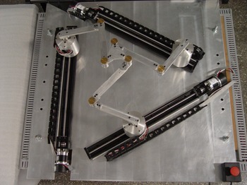
Among the innovative kinematic architectures, the use of actuation or kinematic redundancies may be a suitable alternative for enlarging the usable workspace [Reference Kotlarski, Abdellatif, Ortmaier and Heimann10,Reference Müller and Hufnagel11]. In summary, while actuation redundancy can be implemented by the actuation of passive joints or by the inclusion of active kinematic chains, kinematic redundancy can be implemented by introducing extra active joints in a kinematic chain. In particular, kinematically redundant parallel manipulators not only present reconfiguration capabilities for avoiding singular regions but also may present increased accuracy [Reference Kotlarski, Heimann and Ortmaier12,Reference Jiang, Li, Wang and Chen13], higher motion/force transmissibility [Reference Xie, Liu and Wang14], enhanced dynamic performance [Reference Fontes and da Silva15], and improved energy efficiency [Reference Ruiz, Santos, Croes, Desmet and da Silva16,Reference Abadi, Mahzoon and Farid17]. Figure 1 shows the 3PRRR, a kinematically redundant planar parallel manipulator. The letter R stands for revolute joint and P for prismatic joint, while the underlined letters represent the active joints. This manipulator presents up to three levels of kinematic redundancy depending on the actuation of the prismatic joints.
The prototype 3PRRR: a planar kinematically redundant parallel manipulator.

The inverse kinematic problem of kinematically redundant manipulators admits infinite solutions. The selection of a single solution requires the use of a redundancy resolution scheme that can be solved locally or globally [Reference Siciliano18]. Global approaches, also known as tracking problems, are usually employed to derive optimal inputs for a given trajectory of the manipulator’s end-effector. Several global approaches have been used for solving redundancy resolution problems in the field of parallel manipulators: heuristic-based iterative methods [Reference Fontes, Santos and da Silva19], predictive approaches [Reference Ruiz, Santos, Croes, Desmet and da Silva16,Reference Faroni, Beschi, Tosatti and Visioli20], dynamic programming [Reference Santos and da Silva21], quadratic programming [Reference Hassan, El-Habrouk and Deghedie22], topological analysis [Reference Ferrentino and Chiacchio23], among others. Nevertheless, the control of this kind of manipulator can be a challenging task.
The control of parallel manipulators imposes different challenges than their implementation for serial manipulators [Reference Paccot, Andref and Martinet24]. For instance, joint space control strategies require the calculation of the inverse kinematic model (IKM). Due to their kinematic architecture, this calculation might be cumbersome and time consuming for parallel manipulators. Alternatively, task-space control strategies require measuring the pose of the manipulator’s end-effector that can be done by using vision-based techniques and image processing algorithms [Reference Bellakehal, Andreff, Mezouar and Tadjine25]. A redundant feedback strategy at the joint and task-space level are proposed by ref. [Reference Mohan, Mohanta, Huesing and Corves26] using appropriate sensors. Using this approach, the actual error of the joint displacements are computed, improving the control performance. A similar strategy has been proposed by ref. [Reference Colombo, Fontes and da Silva27] using a rate-limited camera. However, as highlighted by refs. [Reference Paccot, Andref and Martinet24,Reference Colombo, Fontes and da Silva27], these techniques and algorithms must cope with the required sampling time for avoiding delays in the control loops. Both difficulties might yield a lack of performance and stability issues.
Model-based control strategies, which require the derivation of accurate and computationally efficient dynamic models for avoiding stability and performance issues [Reference Di Lillo, Antonelli and Natale28,Reference Coutinho A. and Hess-Coelho29], seem to be superior compared to nonmodel ones [Reference Saied, Chemori, Rafei, Francis and Pierrot8]. These strategies have also been used to overcome the Parallel Manipulators’ drawback related to singular regions [Reference Pagis, Bouton, Briot and Martinet30,Reference Nguyen, Hoang, Go, Kang, Choi, Park and Kim31]. For instance, Pagis et al. [Reference Pagis, Bouton, Briot and Martinet30] propose a multimodel control law that allows parallel manipulators to cross Type 2 singularities, while Nguyen et al. [Reference Nguyen, Hoang, Go, Kang, Choi, Park and Kim31] propose a novel control approach based on the regularization of singular value decomposition (SVD) to solve the singularity problem. Regarding redundantly actuated parallel manipulators, redundancy introduces an infinite number of actuating torque vectors that would satisfy a given task’s requirements. Several model-based control strategies have been proposed to cope with this challenge as reviewed by ref. [Reference Luces, Mills and Benhabib32]. For instance, Muller and Hufnagel [Reference Müller and Hufnagel11] propose a computed torque and augmented PD control scheme using redundant coordinates.
Regarding kinematically redundant parallel manipulators, fewer studies have been reported. A general framework multipriority controller aiming to minimize the execution time and the overall actuator effort is proposed by ref. [Reference Uzunoglu, Tatlicioglu and Dede34]. Two joint space control strategies and global redundancy resolution schemes have been experimentally compared in ref. [Reference Fontes, da Silva and da Silva35]. New insights could be found by evaluating the impact of several levels of kinematic redundancies and different control/redundancy resolution schemes in the field of parallel manipulators. Moreover, not only joint space but also task-space control strategies should be investigated. In this way, this work aims to show that kinematic redundancy can not only be used as an alternative design for reducing the presence of singular regions, as stated in the literature, but also be used along with model-based control strategies for improving dynamic performance and accuracy of parallel manipulators.The evaluation of the impact of several levels of kinematic redundancies and different control/redundancy resolution schemes in parallel manipulators can bring new insights to the field. Moreover, the performance assessment of model-based and model-free control approaches should be addressed. Since their evaluation, along with several kinematic redundancy levels, has not been previously investigated.
In this way, numerical and experimental results on the tracking performance of a planar kinematically redundant parallel manipulator, the 3PRRR (see Fig. 1), are presented and discussed. This performance is assessed by evaluating joint errors, efforts, and repeatability. Three control strategies are evaluated: (i) a nonmodel based joint control strategy (PID), (ii) a model-based joint space CTC, and (iii) a model-based hybrid joint-task computed torque control strategy (HYB). The latter is a novel strategy that requires measuring the end-effector’s pose, which is performed by an eye-to-hand limited frame rate camera. Moreover, the impact of up to three kinematic redundancy levels is evaluated using two global redundancy resolution schemes.
The rest of the manuscript is organized as follows. Section 2 describes the prototype and summarizes the kinematic and dynamic models of the manipulator. While Section 3 introduces the investigated redundancy resolution schemes; Section 4 describes the proposed control strategies. Experimental results are presented and discussed in Section 5. Conclusions are drawn in Section 6.
2. 3PRRR: Prototype and Modeling
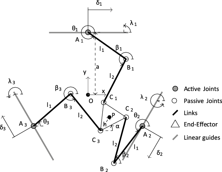
In this section, the prototype 3PRRR is first described (see Fig. 1). Then, the visual system and image processing technique are introduced. Finally, its kinematic and dynamic models are briefly derived for the sake of completeness. Fontes et al. [Reference Fontes and da Silva15] describe these models in detail. The geometric parameters required for the derivation of the kinematic and dynamic models of the 3PRRR manipulator are illustrated in Fig. 2.
2.1. Prototype
Each kinematic chain presents an active prismatic joint (P) and an active revolute joint (R). The actuation of these joints is performed by brushless Maxon EC60 flat motors delivering 100 W of power. These motors are coupled with Maxon planetary gearheads GP52C with a reduction ratio of 3.5:1, resulting in a nominal torque of 0.82 N.m @ 1200 rpm. Table systems with ball screw HIWIN KK60-10-C-E-600-A-1-F0-S3 are responsible for the linear motion. Their stroke range is 600 mm, and their lead is 10 mm. The Maxon EPOS2 50/5 controllers generate the actuation signals and acquire the encoders’ measurements. These signals are processed in a DSpace 1103 acquisition board at a rate of
 $100 \ Hz$
. The communication between the Maxon EPOS2 50/5 controllers and the DSPACE board is performed using CAN protocol. The torques of the active revolute joints,
 $\boldsymbol{\tau}_{\theta}$
, and the active prismatic joints,
 $\boldsymbol{\tau}_{\delta}$
, are proportional to these actuation signals.
In Fig. 2, the subscript
 $i = 1, \ldots, 3$
indicates the kinematic chain. In each kinematic chain, there are one active (
 $A_{i}$
) and two passive (
 $B_{i}$
and
 $C_{i}$
) revolute joints. The angles
 $\theta_{i}$
and
 $\beta_{i}$
represent the orientation of the links
 $A_{i}B_{i}$
and
 $B_{i}C_{i}$
, respectively. Their lengths are
 $l_{1}$
and
 $l_{2}$
, respectively.
Active prismatic joints can modify the position of the point
 $A_{i}$
. By using these linear actuators, the position of
 $A_i$
can be modified according to the position
 $\delta_{i}$
and the orientation
 $\gamma_i$
(
 $\gamma_{i}=\lambda_i-\pi/2$
) of the linear guide. The angular position of the active revolute joints,
 $\boldsymbol{\theta}=[\theta_1,\theta_2,\theta_3]$
, are directly acquired by the encoders, while the position of the active prismatic joints,
 $\boldsymbol{\delta}=[\delta_1,\delta_2,\delta_3]$
, can be derived by using the encoders’ measurements and the lead values.
The distance between the manipulator’s center and the central position of the linear actuators is represented by a. The distance of
 $C_{i}$
to the centre of the end-effector is h. The geometric and inertia values are given in Table. I. The inertia values have been obtained using a model identification procedure in a similar way that was proposed by [Reference Thanh, Kotlarski, Heimann and Ortmaier33]. The following inertia data are used in the dynamic modeling: the mass at the actuator
 $A_i$
is
 $m_0$
, the link
 $A_iB_i$
’s mass and moment of inertia around pivot point
 $A_i$
are
 $m_1$
and
 $I_1$
, the link
 $B_iC_i$
’s mass and moment of inertia around pivot point
 $B_i$
are
 $m_2$
and
 $I_2$
and the end effector’s mass and moment of inertia around the mass center are
 $m_n$
and
 $I_n$
.
Inertial and geometric parameters of the 3PRRR manipulator prototype.

The geometrical parameters of the 3PRRR.

2.2. Visual system and image processing tecnique
The hybrid joint-task CTC strategy requires the measurement of the end-effector’s pose,
 $\mathbf{X}=[x,y,\alpha]^T$
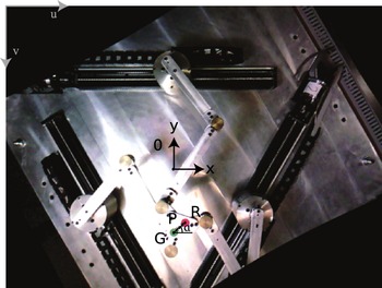
. This strategy is carried out using a limited frame rate camera and image processing algorithms. In an eye-to-hand configuration, a USB 3.0 oCam-5CRO-U colour camera is placed on top of the manipulator, capturing an image frame that is parallel to the planar workspace. As illustrated in Fig. 3, the red and green markers on the end-effector have a significant color difference compared to the rest of the image. Color segmentation is a simple image processing method that can detect objects of a specific color in the image frame, such as the circular markers used. Most color cameras use the RGB (Red, Green, Blue) color space to represent the colors of the pixels by a combination of Red, Green, and Blue. However, for color filtering of an image, a common approach is the conversion to the HSV (Hue, Saturation and Value) colour space since only the Hue channel is needed to describe the pixel’s color. Saturation represents the amount of the color, while Value depends on the lighting conditions. After selecting a range of pixel values in either RGB or HSV color spaces that best describe the color of the object to be detected, the image can be segmented by applying a mask or filter. A binary image with the detected object is created by selecting only the pixels that belong to the range specified.
An image frame used to measure the end-effector’s pose based on the detection of the two colored markers and the coordinate transformation between the uv- and xy-axes.

Two binary images representing the red and green circular markers on the end-effector are extracted. The center of the circles is the average position of all white pixels in each binary image. Geometric relationships between these two points and the end-effector can be used to compute its pose in the image coordinates. The end-effector’s center is the average between the center of the green and red markers (see Fig. 3). The angular position is also easily acquired by considering that the markers’ centers form a parallel line with one side of the end-effector. Although the end-effector’s pose is measured using image-based coordinates, it is possible to convert it into position-based ones, such as the manipulator’s reference system. Since the workspace plane is parallel to the image frame, this coordinate transformation only needs a translation of axes, as seen in Fig. 3. To shift the origin between these coordinate systems, we obtained the manipulator’s coordinates origin in the image frame in a calibration test. For an undistorted image, the corresponding size of a pixel at the workspace plane is used as a scaling factor between these coordinate systems. This algorithm can measure the end-effector’s pose at a sampling time of 60 Hz with an image resolution of 640x480 pixels. Accuracy depends on the relation between in pixel the actual measurement. This is assessed during the system calibration. For the used device, the accuracy is 0.2 mm.
2.3. Kinematic modeling
The IKM is used to determine the active joints inputs
 $\boldsymbol{\Theta} =[\boldsymbol{\theta} \quad \boldsymbol{\delta}]^T= [\theta_{1},\theta_{2},\theta_{3},\delta_{1},\delta_{2},\delta_{3}]^{T}$
that yield a desired end-effector’s pose
 $\mathbf{X} = [x,y,\alpha]^{T}$
. So, considering that a redundancy resolution scheme will define the values of the redundant actuators’ inputs,
 $\boldsymbol{\delta}$
, the inverse kinematics of the manipulator can be derived using the geometrical constraint
 $\left \| \overrightarrow{B_iC_i} \right \| = l_{2}$
, yielding:
 \begin{equation}e_{i1} + e_{i2}\cos(\theta_{i}) + e_{i3}\sin(\theta_{i}) = 0,\end{equation}
where
 $ e_{i1}=-2l_1\rho_{yi}$
,
 $e_{i2}=-2l_1\rho_{xi}$
and
 $e_{i3}=\rho^2_{xi}+\rho^2_{yi}+l^2_1-l^2_2$
. The auxiliary variables are defined by
 $\rho_{xi} = x + h \cos(\alpha+\lambda_{i}) - \delta_i \cos(\gamma_{i}) - a\cos(\lambda_{i})$
and
 $\rho_{yi} = y + h \sin(\alpha+\lambda_{i}) - \delta_i\sin(\gamma_{i}) - a\sin(\lambda_{i})$
, where
 $\gamma_i$
is the orientation of the prismatic joint in the kinematic chain i which can be calculated as
 $\lambda_i -\pi/2$
.
Using the tangent half-angle substitution,
 $\theta_{i}$
is employed to solve Eq. (1) for
 $\theta_{i}$
and can be derived as
 \begin{equation} \theta_i=2\tan^{-1}\left ( \frac{-e_{i1}\pm\ \sqrt{e^2_{i1}+e^2_{i2}-e^2_{i3}}}{e_{i3}-e_{i2}} \right ) \quad \text{and} \quad \beta_i=\tan^{-1}\left ( \frac{\rho_{yi}-l_1\sin(\theta_i)}{\rho_{xi}-l_i\cos(\theta_i)} \right ).\end{equation}
According to the signal choice in Eq. (2), these manipulator presents eight possible working modes. In this work, the plus sign is selected for all calculations yielding the working mode illustrates in Fig. 1.
One way to determine the Jacobian matrix
 $\mathbf{J}$
is by taking the time derivative of the constraint relation described by Eq. (1). The matrix form of this derivation can be written as
 $\mathbf{A}\dot{\mathbf{X}}=\mathbf{B}\dot{\boldsymbol{\Theta}}$
, where the matrices
 $\mathbf{A}$
and
 $\mathbf{B}$
can be defined as
 \begin{equation} \mathbf{A} = \begin{bmatrix} a_{11}\;\;\; & a_{12}\;\;\; & a_{13}\\ a_{21}\;\;\; & a_{22}\;\;\; & a_{23}\\ a_{31}\;\;\; & a_{32}\;\;\; & a_{33} \end{bmatrix} \textrm{ and} \quad \mathbf{B} = \begin{bmatrix} b_{11}\;\;\; & 0\;\;\; & 0\;\;\; & b_{14}\;\;\; & 0\;\;\; & 0\\ 0\;\;\; & b_{22}\;\;\; & 0\;\;\; & 0\;\;\; & b_{25}\;\;\; & 0\\ 0\;\;\; & 0\;\;\; & b_{33}\;\;\; & 0\;\;\; & 0\;\;\; & b_{36}\;\;\; \end{bmatrix}, \end{equation}
where
 $ a_{i1}=l_2\cos(\beta_i)$
,
 $a_{i2}=l_2\sin(\beta_i)$
,
 $a_{i3}=l_2h\sin(\beta_i-\lambda_i-\alpha)$
,
 $b_{ii}=l_1l_2\sin(\beta_i-\theta_i)$
and
 $b_{i i+3}=l_2\cos(\beta_i-\gamma_i)$
. The Jacobian matrix can be defined as
 $ \mathbf{J}=\mathbf{A}^{-1}\mathbf{B}$
.
2.4. Dynamic modeling
The dynamic model of the manipulator is derived in this section using the Newton–Euler formulation and the previously described kinematics. According to Table I, the subscripts
 $j=0,1,2$
are related to the actuator
 $A_i$
, link
 $A_iB_i$
and link
 $B_iC_i$
, while n is related to the end-effector.
The relation between the generalized efforts
 $\boldsymbol{\tau}=[\boldsymbol{\tau}_{\theta} \quad \boldsymbol{\tau}_{\delta}]^T$
applied by the actuators and the forces and moments on the system are expressed with the Principle of Virtual Work [Reference Wu, Wang and You36]. This relation uses the components of the vector
 $\mathbf{p}_{ij}$
, which are composed by the combination of forces and moment applied on the body j of the chain i; the displacement vector
 $\mathbf{d}_{ij}=[r_{x_{ij}} \quad r_{y_{ij}} \quad \phi_{ij}]^T$
; and the components of the vector
 $\mathbf{p}_{n}$
composed by the forces and moment applied on the end-effector. Since the dynamic model is defined using virtual work, it is necessary to obtain Jacobian matrices
 $\mathbf{K}_{ij}$
for each moving body of the manipulator. The detailed definition for these matrices can be found in [Reference Fontes and da Silva15]. This strategy yields the following relation:
 \begin{equation} \boldsymbol{\tau}=\mathbf{J}^T\mathbf{p_n} +\sum_{i=1}^{3}\sum_{j=0}^{2}\mathbf{K_{ij}}^T\mathbf{p_{ij}}.\end{equation}
The vectors
 $\mathbf{p_{ij}}$
and
 $\mathbf{p_n}$
can be described:
 \begin{equation}\mathbf{p_{ij}}=\mathbf{Z_{ij}} \begin{bmatrix} \ddot{r}_{x_{ij}}\\[3pt] \ddot{r}_{y_{ij}}\\[3pt] \ddot{\phi}_{ij} \end{bmatrix}+ \mathbf{N_{ij}} \begin{bmatrix} \dot{r}_{x_{ij}}\\[3pt] \dot{r}_{y_{ij}}\\[3pt] \dot{\phi}_{ij} \end{bmatrix} \quad \text{and} \quad \mathbf{p_n}=\mathbf{Z_n}\begin{bmatrix} \ddot{x}\\[3pt] \ddot{y}\\[3pt] \ddot{\alpha} \end{bmatrix}\end{equation}
where
 \begin{equation}\mathbf{Z_{ij}}=\begin{bmatrix} m_j & 0 & \;\;-m_j s_{ij}\sin{\phi_{ij}} \\ 0 & m_j & \;\;m_j s_{ij}\cos{\phi_{ij}} \\ -m_j s_{ij}\sin{\phi_{ij}}\;\;\;\; &m_j s_{ij}\cos{\phi_{ij}}\;\;\;\; & I_j \end{bmatrix},\end{equation}
 \begin{equation}\mathbf{N_{ij}}=\begin{bmatrix} 0\;\;\; & 0\;\;\; & -m_j \dot{\phi}_{ij} s_{ij}\cos{\phi}_{ij} \\[3pt] 0\;\;\; & 0\;\;\; & -m_j \dot{\phi}_{ij} s_{ij}\sin{\phi}_{ij} \\[3pt] 0\;\;\; & 0\;\;\; & 0\end{bmatrix} \quad \text{and} \quad \mathbf{Z_{n}}=\begin{bmatrix} m_n\;\;\; & 0\;\;\; & 0 \\ 0\;\;\; & m_n\;\;\; & 0 \\ 0\;\;\; & 0\;\;\; & I_n \end{bmatrix}\end{equation}
These equations can be rewritten in term of the time derivatives of
 $\boldsymbol{\Theta}$
using the Jacobian matrices yielding:
 \begin{equation} [\tau_1 \quad \tau_2 \quad \tau_3 \quad \tau_4 \quad \tau_5 \quad \tau_6 ]^T= \mathbf{M}\ddot{\boldsymbol{\Theta}}+\mathbf{V}\dot{\boldsymbol{\Theta}},\end{equation}
where:
 \begin{equation} \mathbf{M}=(\mathbf{J}^T\mathbf{Z_n}\textbf{J} +\sum_{i=1}^{3}\sum_{j=0}^{2}\mathbf{K_{ij}}^T\mathbf{Z_{ij}}\mathbf{K_{ij}}) \quad \text{and}\end{equation}
 \begin{equation} \mathbf{V}=(\mathbf{J}^t\mathbf{Z_n}\mathbf{{J}} +\sum_{i=1}^{3}\sum_{j=0}^{2}\mathbf{K_{ij}}^T\mathbf{Z_{ij}}\mathbf{{K}_{ij}}+\sum_{i=1}^{3}\sum_{j=0}^{2}\mathbf{K_{ij}}^t\mathbf{N_{ij}}\mathbf{K_{ij}}).\end{equation}
Since
 $\tau_4$
,
 $\tau_5$
, and
 $\tau_6$
are generalized forces, they must be converted to torque using the lead K of the linear guide leading to
 \begin{equation} \boldsymbol{\tau}= [\boldsymbol{\tau}_{\theta} \quad \boldsymbol{\tau}_{\delta}]^T = [\tau_1 \quad \tau_2 \quad \tau_3 \quad K\tau_4/(2\pi) \quad K\tau_5/(2\pi) \quad K\tau_6/(2\pi)]^T\end{equation}
It is important to highlight that the dynamic model depends on the angles
 $\phi_{ij}$
. These angles are defined as 0 for
 $j=0$
,
 $\theta_i$
for
 $j=1$
and
 $\beta_i$
for
 $j=2$
. This dependency is critical for the control strategies based on the model, since
 $\beta_i$
can only be analytically calculated by the IKM.
3. Redundancy Resolution
Redundancy resolution is a decision-maker strategy used for deriving the position of the redundant joints among the possibilities. This strategy can be mathematically described as an optimization problem. Some redundancy resolution schemes seek to minimize the maximum required torque to perform a predefined task. However, this approach does not guarantee the avoidance of singular regions during the task execution.
In this work, a multiobjective optimization problem is adopted to overcome this issue. In the proposed approach, the minimization of the required torque is considered and the avoidance of the singular regions. In this way, two functions are defined,
 $\upsilon_1$
and
 $\upsilon_2$
whose values present a strong relation with the distance from the type 1 and type 2 singularities, respectively. According to Pagis et al., type 1 singularities occur when the mechanism is unable to move in a given direction due to the rank deficiency of the kinematic matrix
 $\mathbf{B}$
(Eq. (3)), and type 2 singularities occur when one or more of the manipulator’s degrees of freedom become uncontrollable due to the rank deficiency of the kinematic matrix
 $\mathbf{B}$
(Eq. (3)). In this way, penalty functions are proposed for guaranteeing the avoidance of types 1 and 2 singularities.
First, a function
 $\upsilon_1$
is proposed for the avoidance of type 1 singularities. These singularities can be avoided by assuring that the values of
 $\sin(\beta_i-\theta_i)$
, from Eq. (12), are positive. Equation 12 only considers the nonredundant part of the matrix
 ${\mathbf{B}}$
(see Eq. (3)) in the following way:
 \begin{equation} \mathbf{B}' = \begin{bmatrix} l_1l_2\sin(\beta_1-\theta_1)\;\;\; & 0 & 0\\ 0 & l_1l_2\sin(\beta_2-\theta_2)\;\;\; & 0\\ 0 & 0 & l_1l_2\sin(\beta_3-\theta_3) \;\;\; \end{bmatrix}.\end{equation}
Considering that the singular values of
 $\mathbf{B}'$
are related to
 $\sin(\beta_i-\theta_i)$
, the avoidance of type 1 singularity can be guaranteed by maximizing the smallest singular value of
 $\mathbf{B}'$
. Since the smallest singular value varies in time during the task execution, the minimum value of the smallest singular values (worst case) is considered in the optimization problem. In this way, the function
 $\upsilon_1$
is defined by
 \begin{equation} \upsilon_1 = min \quad \frac {min \ \nu(\mathbf{B}')}{l_1l_2},\end{equation}
where
 $\nu(\mathbf{B}')$
are the singular values of matrix
 $\mathbf{B}'$
, and
 $l_1$
and
 $l_2$
are used for normalizing the relation. The value of
 $\upsilon_1$
varies between 0 and 1 and should be maximized for guaranteeing the avoidance of type 1 singularity.
Second, a function
 $\upsilon_2$
is proposed for the avoidance of type 2 singularities. This requirement can be assessed by evaluating indices derived from the Jacobian matrix
 $\mathbf{A}$
[Reference Alba-Gomez, Wenger and Pamanes37]. For the manipulator under study, the Jacobian matrix
 $\mathbf{A}$
(see Eq. (3)) is not homogeneous and, therefore, the indices defined directly from it have no physical meaning. To overcome this problem, the Jacobian matrix
 $\mathbf{A}$
could be normalized using the characteristic length of the manipulator, given by
 $Lc = \sqrt{2}h $
[Reference Alba-Gomez, Wenger and Pamanes37,Reference Reveles, Pamanes and Wenger38]. This normalization can be applied to the angular-related elements of the matrix
 $\mathbf{A}$
yielding the normalized matrix:
 \begin{equation} \mathbf{{A}}' = \begin{bmatrix} a_{11}\;\;\; & a_{12}\;\;\; & a_{13}/Lc\\ a_{21}\;\;\; & a_{22}\;\;\; & a_{23}/Lc\\ a_{31}\;\;\; & a_{32}\;\;\; & a_{33}/Lc \end{bmatrix}.\end{equation}
The distance between the end-effector and the singularities of type 2 is related to the conditioning number of the normalized Jacobian matrix
 ${\mathbf{A}}'$
defined by
 \begin{equation} \kappa({\mathbf{A}}')=\frac{max\ \nu({\mathbf{A}}')}{min\ \nu({\mathbf{A}}')}.\end{equation}
where
 $\nu({\mathbf{A}}')$
are the singular values of the matrix
 ${\mathbf{A}}'$
. Since
 $\kappa({\mathbf{A}}')$
varies in time during the task execution, its maximum value is going to be considered in the cost function. In this way, the function
 $\upsilon_2$
is defined by
 \begin{equation} \upsilon_2 = max \quad \kappa({\mathbf{A}}').\end{equation}
The value of
 $\nu({\mathbf{A}}')$
varies from 1 to
 $\infty$
. The higher the value of
 $\nu({\mathbf{A}}')$
, the nearer to a singularity the end-effect is. In this way, the avoidance of type 2 singularity can be guaranteed by minimizing the
 $\upsilon_2$
.
The proposed multiobjective optimization problem seeks to minimize the maximum required torque (
 $\left \| \boldsymbol{\tau} \right \|_\infty$
), to maximize the function
 $\upsilon_1$
for avoiding type 1 singularities and to minimize the function
 $\upsilon_2$
for avoiding type 2 singularities. A weighted sum strategy is proposed to convert this multiobjective problem into a single optimization problem defined by
 \begin{equation} F_{cost} = \left \| \boldsymbol{\tau} \right \|_\infty + w[\upsilon_2 - \upsilon_1],\end{equation}
where w is a weighting factor. The definition of this objective function yields the following nonlinear constrained optimization problem:
 \begin{equation} \begin{split} \delta_{i,opt}(t) = arg &\quad min_{\ \delta_i(t)} \ F_{cost} \\ subject \ to\;:\;\ \delta_{min}&\leq\delta_i(t)\leq\delta_{max}\\ \upsilon_1 &\geq R_1 \\ \upsilon_2 &\leq R_2\end{split}\end{equation}
where
 $R_1$
and
 $R_2$
are the lower and upper bounds selected to keep the end-effect far enough from the singularities.
The variables of this optimization problem should describe the inputs for the redundant actuators
 $\delta_i(t)$
. Since the inputs
 $\delta_i(t)$
are time-dependent variables, they cannot be directly used as optimization variables. Thus, two different approaches are explored to represent these variables: prepositioning and ongoing positioning approaches [Reference Kotlarski, Abdellatif, Ortmaier and Heimann10].
On the one hand, the prepositioning approach consists of determining the optimal inputs for the redundant active prismatic joints before the execution of the task (the predefined trajectory). In this way, the positions of the active prismatic joints (the linear guides), denoted as
 $\delta_ {fixed_i,opt}$
, are the same throughout the execution of the task. Therefore, this optimization problem can be described as
 \begin{equation} \begin{split} \delta_{fixed_i,opt} = arg &\quad min_{\ \delta_{fixed_i}} \ F_{cost} \\ subject \ to\;:\;\ \delta_{min}&\leq\delta_{fixed_i}\leq\delta_{max}\\ \upsilon_1 &\geq R_1 \\ \upsilon_2 &\leq R_2 \end{split}\end{equation}
On the other hand, the ongoing positioning approach consists of determining the optimal inputs for the redundant active joints considering that they can also move during the execution of the task (the predefined trajectory). A fifth-order polynomial for describing these inputs have been selected. For deriving the coefficients of this polynomial, the initial and final positions, velocities, and accelerations should be known. The initial and final velocities and accelerations are equal to zero. So, the optimization variables are the values of the initial (
 $\delta_{0_i,opt}$
) and final (
 $ \delta_{f_i,opt}$
) positions of the active prismatic joints (the linear guides). Therefore, this optimization problem can be described as
 \begin{equation} \begin{split} [{\delta_{0_i,opt},\delta_{f_i,opt}}] = arg &\quad min_{\ [\delta_{0_i},\delta_{f_i}]} \ F_{cost} \\ subject \ to\;:\;\delta_{min}&\leq\delta_{0_i}\leq\delta_{max} \\ \delta_{min}&\leq\delta_{f_i}\leq\delta_{max} \\ \delta_{min}&\leq\delta_{i}\leq\delta_{max} \\ \upsilon_1 &\geq R_1 \\ \upsilon_2 &\leq R_2\end{split}\end{equation}
Both redundancy resolution schemes are performed offline, which means that they must be executed before the experiment. They are solved by using a hybrid optimization strategy. A classical genetic algorithm (GA) is used for delivering good initial guesses for Sequential Quadratic Programming (SQP), which is responsible for providing refined results. This strategy has been able to provide satisfactory results on reasonable processing time. The outcome of this optimization is the desired positions for the active redundant actuators (the active prismatic joints) which is denoted as
 $\boldsymbol{\delta}_d(t)$
. The values of
 $\boldsymbol{\delta}_d(t)$
are used as the references for the control strategies.
4. Control Strategies
For a predefined trajectory
 $\mathbf{X}_d$
, a set of desired positions for the active redundant joints
 $\boldsymbol{\delta}_d$
can be derived by one of the redundancy resolution schemes (Eqs. (19) or (20)). The desired positions of the active nonredundant joints
 $\boldsymbol{\theta}_d$
can be derived by using the IKM, described in Section 2.3, for given values of
 $\mathbf{X}_d$
and
 $\boldsymbol{\delta}_d$
. For a given
 $\boldsymbol{\Theta}_d =[\boldsymbol{\theta}_d \quad \boldsymbol{\delta}_d]^T$
, the required torque to be applied in the manipulator is derived using three control strategies in this work. These strategies are experimentally implemented and compared.
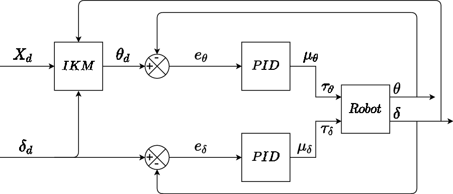
The first strategy is a model-free independent PID joint control scheme. This strategy is illustrated in Fig. 4. The desired positions of the active joints,
 $\boldsymbol{\theta}_d$
and
 $\boldsymbol{\delta}_d$
, are used as reference signals in the control loop. These signals are compared with the actual measurement,
 $\boldsymbol{\theta}$
and
 $\boldsymbol{\delta}$
, and the differences between these signals,
 $\boldsymbol{e}_{\theta}=\boldsymbol{\theta}_d-\boldsymbol{\theta}$
and
 $\boldsymbol{e}_{\delta}=\boldsymbol{\delta}_d-\boldsymbol{\delta}$
, are the inputs for the PID controls. Different gains are used for the actuators responsible for the motion of the active revolute (nonredundant) and prismatic (redundant) joints. These gains have been experimentally adjusted by a trial-and-error method. The torque calculated using this strategy,
 $\boldsymbol{\tau}_{PID}$
, can be calculated using the following control law:
The independent PID joint control scheme (PID).

 \begin{equation} \boldsymbol{\tau}_{PID} = [\boldsymbol{\tau}_{\theta}, \ \boldsymbol{\tau}_{\delta}]=K_p\mathrm{e}+K_d\frac{\mathrm{d} e}{\mathrm{d} t}+K_i\int_{0}^{t}e \ \mathrm{d}\rho\end{equation}
where
 $\boldsymbol{e} = [\boldsymbol{e}_{\theta},\boldsymbol{e}_{\delta}$
],
 $\boldsymbol{K}_p$
,
 $\boldsymbol{K}_d$
and
 $\boldsymbol{K}_i$
are the proportional, derivative and integral gains.
The second strategy is a joint space CTC scheme. Figure 5 shows a scheme of the second strategy. In this strategy, a feedforward signal is added since an inverse dynamic model (IDM), derived in Section 2.4, is available. Based on the IKM, the desired joint positions
 $[\boldsymbol{\theta}_d, \boldsymbol{\delta}_d]$
, velocities
 $[\dot{\boldsymbol{\theta}}_d, \dot{\boldsymbol{\delta}}_d]$
and accelerations
 $[\ddot{\boldsymbol{\theta}}_d, \ddot{\boldsymbol{\delta}}_d]$
are derived. Moreover, the desired angular positions of the passive joints
 $\boldsymbol{\beta}_d$
are also derived using Eq. (2). These desired values are used in the Eq. (4) to compute the required torque to the task execution (the feedforward signal):
The CTC strategy.

 \begin{equation} \boldsymbol{\tau}_{ff}=[\boldsymbol{\mu}_{ff\theta}, \ \boldsymbol{\mu}_{ff\delta}] =\text{IDM}(\boldsymbol{\beta}_d,\boldsymbol{\theta}_d,\dot{\boldsymbol{\theta}}_d,\ddot{\boldsymbol{\theta}}_d,\boldsymbol{\delta}_d,\dot{\boldsymbol{\delta}}_d,\ddot{\boldsymbol{\delta}}_d)\end{equation}
This computed torque (feedforward signal) may enhance the system performance regarding the tracking reference and disturbance rejection capabilities since it might compensate for Coriolis, centrifugal, frictional forces, among others. Nevertheless, the PID scheme is also used in this strategy for robustness since the dynamic model is surely imprecise. This CTC strategy yields the following control law:
 \begin{equation} \boldsymbol{\tau}_{CTC} = [\boldsymbol{\tau}_{\theta}, \ \boldsymbol{\tau}_{\delta}]=[\boldsymbol{\mu}_{ff\theta}+\boldsymbol{\mu}_{\theta}, \ \boldsymbol{\mu}_{ff\delta}+\boldsymbol{\mu}_{\delta}]\end{equation}
where
 $\boldsymbol{\mu}_{\theta}$
and
 $\boldsymbol{\mu}_{\delta}$
are the output of the PID controllers as can be seen in Fig. 5.
The third strategy is a hybrid joint-task space CTC strategy. Figure 6 shows a scheme of the third strategy. While the computed torque is derived using the desired kinematic quantities (Eq. (22)) in the second control strategy, the actual measurements will be used in the control loops in the third control strategy. Not only the actual positions of the nonredundant and redundant actuators,
 $\boldsymbol{\delta}$
and
 $\boldsymbol{\theta}$
(joint space), but also the actual positions of the end-effector,
 $\boldsymbol{X}$
(task space), are used. The task space is measured using a camera and image processing algorithms (see Section 2.1).
The Hybrid Joint-Task Space computed torque control strategy (HYB).

The hybrid joint-task space CTC strategy, illustrated in Fig. 6, presents two control loops: an internal loop that considers the dynamic model and an external loop that tracks the error. For these loops, kinematic quantities are required. The first- and second-time derivatives of the actual actuators’ positions are calculated using derivative blocks and estimated signals. The estimated second-time derivative of the nonredundant actuators’ positions are calculated by
 \begin{equation} \ddot{\boldsymbol{\theta}}_*=\ddot{\boldsymbol{\theta}}_d+\boldsymbol{u}_{\theta}\end{equation}
where
 $\boldsymbol{u}_{\theta}$
is the outcome of PID blocks while the vector of errors of the actuators’ positions (
 $\boldsymbol{e}_{\theta}=\boldsymbol{\theta}_d-\boldsymbol{\theta}$
) is the input. The same approach is used for estimating the second-time derivative of the redundant actuators’ positions,
 $\ddot{\boldsymbol{\delta}}_*$
.
The computed torque is calculated using the IDM, which requires not only the actuators’ positions but also the angle of the passive joints
 $\boldsymbol{\beta}$
. Using the IKM, the actual angular positions of the passive joints
 $\boldsymbol{\beta}$
can be also estimated using the actual positions of the active joints,
 $\boldsymbol{\theta}$
, and of the end-effector,
 $\boldsymbol{X}$
(see Eq. (2)). In this way, these states are used as input signals along with the kinematic quantities of the actuators. In summary, the required torque for executing a task is derived using not only the IKM and the IDM but also the actual and estimated kinematic quantities:
 \begin{equation} \boldsymbol{\tau}_{HYB} = [\boldsymbol{\tau}_{\theta}, \ \boldsymbol{\tau}_{\delta}] = \text{IDM}(\boldsymbol{\beta},\boldsymbol{\theta},\dot{\boldsymbol{\theta}},\ddot{\boldsymbol{\theta}}_*,\boldsymbol{\delta},\dot{\boldsymbol{\delta}},\ddot{\boldsymbol{\delta}}_*)\end{equation}
Both second and third strategies require the calculation of the inertia matrix and the Coriolis vector. These three control strategies are implemented in a Simulink model, compiled for a dSPACE 1103 board. The strategies use the same PID gains for the sake of comparison. In the next section, these strategies are compared considering the RMS (root mean square) of the error vectors (
 $\boldsymbol{e}_{\theta}=\boldsymbol{\theta}_d-\boldsymbol{\theta}$
and
 $\boldsymbol{e}_{\delta}=\boldsymbol{\delta}_d-\boldsymbol{\delta}$
) and the RMS of the torques (
 $\boldsymbol{\tau}_{\theta}$
and
 $\boldsymbol{\tau}_{\delta}$
).
5. Results
In this section, the impact of up to three levels of kinematic redundancy of the planar parallel manipulator 3PRRR is numerically and experimentally evaluated. This evaluation is carried out for two redundancy resolution schemes: the prepositioning approach (PRE - Eq. (19)) and the ongoing positioning approach (ON - Eq. (20)); and for three control strategies: the model-free control (PID - Eq. (21)), the joint space CTC (CTC - Eq. (23)), and the hybrid joint-task space computed torque control (HYB - Eq. (25)) strategies.
For the sake of comparison, the same task is performed for all possible configurations under evaluation. This task is characterized by a point-to-point straight-line trajectory. The initial and the final points are given by
 $\mathbf{X}_d^{initial} = [0.09\ \mathrm{m}, -0.03\ \mathrm{m}, 0.2\ rad]$
and
 $\mathbf{X}_d^{final}$
= [
 $-0.09$
m,
 $0.03$
m,
 $0.1$
rad], respectively. The task duration is 1s, and during its execution, the end-effector pass near a singular region. This task is mathematically described using a fifth-degree polynomial considering initial and final velocities and accelerations equal to zero.
For a given trajectory,
 $\mathbf{X}_d$
, the redundancy resolution schemes are responsible for deriving the inputs for the redundant actuators
 $\boldsymbol{\delta}_d$
. These schemes require the definition of the constraint parameters and weighting factor (Eqs. (19) and (20)). The linear guides must not reach their mechanical limits yielding the following bounds:
 $\delta_{min}=-0.23$
m and
 $\delta_{max}=0.23$
m. The end-effector must stay far enough from the singularities. This can be guaranteed by setting
 $ R_1=2$
and
 $R_2 = 0.45$
. Finally, the weighting factor w was defined as
 $ 0.02 $
, which prioritizes the minimization of the maximum required torque to perform the trajectory. This choice is carried out from a trial-and-error approach. This prioritization can be applied due to the proper selection of
 $R_1$
and
 $R_2$
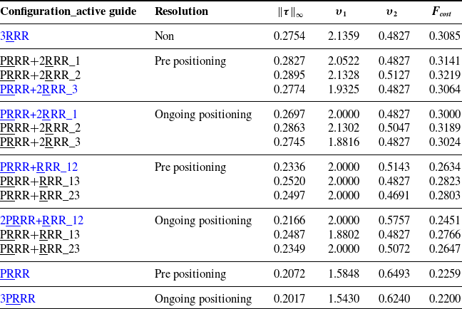
. Table II shows the values of the objective functions for the nonredundant and redundant manipulators using different redundancy resolution schemes.
Maximum torque values, singularities indexes and cost function for the nonredundant and redundant manipulators using different redundancy resolution schemes

Since the manipulator presents up to three levels of kinematic redundancies, the activation of these redundancies can be done in different ways. For instance, for a single level of kinematic redundancy (PRRR+2RRR), one can activate the linear guide 1 without activating the other two (PRRR+2RRR_1 in Table II), or activate only the linear guide 2 or only the linear guide 3 (PRRR+2RRR_2 and PRRR+2RRR_3, respectively). In the same way, this occurs for two levels of kinematic redundancy, activating the linear guides 1 and 2, or 1 and 3, or 2 and 3 (PRRR+2RRR_12, PRRR+2RRR_13 and PRRR+2RRR_23, respectively). The redundancy resolution schemes have been solved for all possible combinations as shown in Table II.
It can be noted that the lowest objective function value was obtained by the redundant manipulator 3PRRR and the ongoing positioning redundancy resolution scheme. Within each possible combination of redundancy resolution level and scheme, the best configurations are the PRRR+2RRR_3 with prepositioning, the PRRR+2RRR_1 with ongoing positioning, the 2PRRR+RRR_12 with prepositioning and ongoing positioning schemes.
Considering the best configurations within each level and redundancy resolution scheme, it can be noted that the higher the level of kinematic redundancy, the lower the objective function. Comparing the same level of kinematic redundancy, the ongoing positioning redundancy resolution scheme presented a better performance for all configurations. Furthermore, comparing the best case (3PRRR with ongoing positioning) with the worst case (3RRR), there was a reduction of 26% in the maximum torque to perform the same task. In addition, better singularities indices were obtained when three levels of kinematic redundancy were used. This numerical comparison indicates that it is possible to improve the dynamic performance of this manipulator and, at the same time, keep the end-effector away from singularities by using kinematic redundancies.
Based on these numerical results, experiments have been conducted for the configurations presenting the lowest objective function value for each kinematic redundancy level and redundancy resolution scheme. These configurations are highlighted in blue in Table II. In this experimental campaign, the desired trajectory was performed ten times to assess the accuracy of the procedure and improve the reliability of the data. The means and confidence intervals were calculated with a 95 % confidence level.
Figures 7 and 8 show the RMS of
 $\boldsymbol{e}_{\theta}$
and
 $\boldsymbol{e}_{\delta}$
and their confidence interval for the nonredundant manipulator and for the best configurations of the redundant manipulators. The confidence interval is quite small demonstrating the data accuracy.
RMS of
 $\boldsymbol{e}_{\theta}$
: a comparison between the PID, CTC and HYB control strategies.

RMS of
 $\boldsymbol{e}_{\delta}$
: a comparison between the PID, CTC and HYB control strategies.

The model-based control strategies (CTC and HYB) obtained smaller errors when compared with the model-free control strategy (PID), as shown in Fig. 8. Moreover, the ongoing positioning scheme presented higher errors when used along with the PID control strategy, demonstrating that model-based control strategies deliver superior results for this prototype. Regarding the model-based control strategies, the CTC strategy obtained smaller errors when compared with the HYB strategy. The main reason for this outcome is probably related to the camera rate limitation reducing the control bandwidth of the HYB strategy. Comparing the best case (3PRRR with ongoing positioning scheme and CTC control strategy) with the worst case (3RRR with PID control strategy), there was a reduction of 72 % in the RMS of
 $\boldsymbol{e}_{\theta}$
to perform the same task.
Figure 9 shows the RMS of the error of the angular position of the end-effector (
 $\alpha_d-\alpha$
) and their confidence interval for the nonredundant manipulator and for the best configurations of the redundant manipulators. This figure shows that the error of the end-effector’s angular position plays an important role in the total error in the task space. These results might indicate the importance of improving the measurements of the task space for further enhancing the prototype’s accuracy. This can also be observed in Fig. 10. This figure shows the x-y and
 $\alpha$
values of the desired trajectory, the trajectory performed by the 3RRR with PID control strategy (Non/PID), and the trajectory performed by the 3PRRR with prepositioning redundancy resolution scheme and CTC control strategy (Prep/CTC). One can observe that both strategies could guarantee the desired angular position of the end-effector at the end of the task execution (1 s). Moreover, it is important to notice that gravitational forces in both control schemes cause a steady error.
RMS of the error of the angular postion fo the end-effector (
 $\alpha_d-\alpha$
): a comparison between PID, CTC and HYB control strategies.

Comparison between the desired trajectory (desired) and (a) the x and y positions and (b) the
 $\alpha$
angular position of the end-effector considering the 3RRR/PID control strategy (Non/PID) and the 3PRRR using the prepositioning redundancy resolution scheme/CTC control strategy (Prep/CTC).

Figure 11 shows the maximum absolute of
 $\boldsymbol{\tau}$
and confidence interval for the nonredundant manipulator and the best configurations of the redundant manipulators. One can realize that a substantial reduction of the maximum required torque could be achieved by using two or three levels of kinematic redundancy and model-based control strategies. Both redundancy resolution schemes were capable of promoting this reduction. The most significant decrease was achieved by two levels of kinematic redundancies using the prepositioning redundancy resolution scheme. The main reason for this outcome is probably related to the differences between friction coefficients of the linear guides. Comparing the best case (2PRRR+RRR_12 with ongoing positioning scheme and CTC control strategy) with the worst case (3RRR with PID control strategy), there was a reduction of 47 % in the maximum torque to perform the same task.
Maximum absolute of
 $\boldsymbol{\tau}$
: a comparison between the PID, CTC and HYB control strategies.

These experimental results indicate that it is possible to improve the dynamic performance and, at the same time, improve the task-space accuracy of this manipulator by using kinematic redundancies and model-based control strategies.
6. Conclusions
In this work, the impact of up to three levels of kinematic redundancy of the planar parallel manipulator 3PRRR is numerically and experimentally evaluated. This evaluation is carried out for two redundancy resolution schemes: the prepositioning and the ongoing positioning approaches and for three control strategies: the model-free control, the joint space CTC, and the hybrid joint-task space CTC strategies.
Due to the presence of kinematic redundancies, several configurations could be investigated by activating the redundant actuators. Both redundancy resolution schemes have been numerically investigated for all possible configurations. The same task has been simulated for the sake of comparison. The numerical results indicated that the ongoing strategy applied for the 3PRRR was capable of reducing the maximum required torque by 26% when compared with the nonredundant manipulator. This numerical result indicates that it is possible to improve the dynamic performance of this manipulator and, at the same time, keep the end-effector away from singularities by using kinematic redundancies.
Based on these numerical results, experiments have been conducted for the configurations presenting the lowest objective function value for each kinematic redundancy level and redundancy resolution scheme. The experimental results showed that a reduction of 72% in the RMS value of the end-effector’s tracking error was achieved by using the ongoing positioning redundancy resolution scheme for the 3PRRR along with the joint space CTC strategy. Moreover, the experimental results showed that a reduction of 47% in the maximum required torque was achieved using the ongoing positioning redundancy resolution scheme for the 2PRRR+RRR along with the joint space CTC strategy.
These numerical and experimental results indicate that it is possible to improve not only the dynamic performance but also the task-space accuracy of this manipulator by using extra levels of kinematic redundancies and model-based joint and task space control strategies. It is important to highlight that this conclusion should be further investigated by evaluating other trajectory and performance indexes.
Finally, it was expected that the hybrid joint-task space CTC strategy would present the best results because it explores the actual positions of the joints. However, some limitations have been identified by the use of a limited rate-frame camera. The hybrid joint-task space CTC strategy could be improved for future works if an appropriate rate-frame camera is used. Moreover, the accuracy can be further enhanced if strategies for avoiding gravitational errors were applied.
Acknowledgments
This research is supported by FAPESP 2018/21336-0 and CNPq 405569/2016-5. Moreover, Maíra M. da Silva, Fernanda T. Colombo, and Joao V. C Fontes are grateful for their research grants, CNPq 301338/2018-3, FAPESP 2018/22760-0, and CNPq 140561/2015-3, respectively. Natassya Silva acknowledges the support granted by UTFPR.
Competing Interests
The authors declare none.