Generalization, External Validity, Replication, and Reproduction

In this article, we focus on techniques for generating evidence in support of the generalizability of an empirical model of a data-generating process, which is a function mapping explanatory variables to outcomes estimated from data which describes how the data could have arisen. We argue that generalization is similar to external validity, which can be supported by replication, but which is not possible in cases where the process generating the data is not under researcher control.

Though the terms generalizability and external validity are often used synonymously with one another, the statistical learning community defines generalizability differently than how Shadish (2010) defines external validity.Footnote ⁵ Generalization in the statistical learning sense refers to the transportability of a learned function (i.e., one estimated from data) to other draws from the same data-generating process, and is focused explicitly on prediction. A learned function that generalizes well has low prediction error on new data from the same generating process. Generalization error is not an estimate of the validity of cause–effect relationships (internal validity), which may or may not be plausibly causally identified in a model fit to observational or quasi-experimental data (see e.g., Dunning Reference Dunning2012; Keele Reference Keele2015; Keele and Titiunik Reference Keele and Titiunik2015 for more general discussions of causal identification in the social sciences).Footnote ⁶ Neither is generalizability in this sense external validity, since the latter pertains explicitly to the generalizability of cause–effect relationships learned from data.

Shadish defines external validity as the “validity of inferences about whether the cause-effect relationship holds over variation in persons, settings, treatment variables, and measurement variables” or outcome variables (2010, 4). These components make up a theoretically specified data-generating process and are linked together by a set of assumptions (premises or postulates) and a set of propositions. These assumptions and propositions link the treatment or causal variable (X) to a measurement or outcome variable (Y) within a specified empirical domain. The domain within which the theory explains the relationship between the treatment and outcome variables is bounded by scope conditions. The scope conditions of a theory are auxiliary assumptions, specifically regarding the attributes of the persons (i.e., the units) and the settings within which the persons reside (i.e., the spatial and temporal information). This auxiliary information is important because a data-generating process might change systematically for different types of persons or units (e.g., Brady Reference Brady1986; Wilcox, Sigleman and Cook 1989; King et al. Reference King, Murray, Solomon and Tandon2004), or across time or between places (e.g., Western Reference Wilcox, Sigleman and Cook1998; Bailey Reference Bailey2007; Fariss Reference Fariss2014).

If theoretical differences between data-generating processes are not recognized and specified in the empirical model (e.g., by including important covariates capturing structural change) of said data-generating process then any predictions from the model will be biased (see e.g., Fariss Reference Fariss2014; Fariss Reference FarissForthcoming, for a discussion of this issue as it relates to the study of human rights).Footnote ⁷ Thus, the scope conditions of the theory provide important information about the conditions that must be met in order for the model of the data-generating process to be a valid representation of the theory (e.g., Adcock and Collier Reference Adcock and Collier2001; Lake Reference Lake2013; Elkins and Sides Reference Elkins and Sides2014; Fariss Reference Fariss2014). To reiterate, generalizability or generalization error is an estimate of the ability of a model to generate accurate predictions on new data from a data-generating process. In practice, what distinguishes one data-generating process from another is the scope or the domain of the theory (e.g., Lake Reference Lake2013).Footnote ⁸ The importance of specifying the scope conditions of a theory is essential because multiple and related data-generating processes may be operating on different units or across different spatial or temporal settings. The generalization error of a model provides important information about how well the learned function generalizes to the data-generating process under study but not necessarily any other data-generating processes. Stated differently, generalization error does not necessarily provide information about the performance of a model on a sample drawn from a different population or using different treatment or outcome variables, except insofar as a different populations or measurements are similar to the process that generated the data used to fit the model (Bareinboim and Pearl Reference Bareinboim and Pearl2012). In this way the definition of generalization error is analogous to exact replication because neither generalization error nor exact replication pertain to the transportability of a model of one data-generating process to another, but both pertain to the reliability of estimates: predictions and treatment effects, respectively.

Shadish (2010) makes a similar point about the external validity of causal inferences: exact replication provides evidence for the external validity of an inference only when the sample (i.e., the persons or settings) and the explanatory variables (i.e., the component parts of a theoretically specified data-generating process) are fixed or at least probabilistically equivalent once accounting for measurement error. However, the external validity of a causal inference can also be enhanced by varying one or more of these components of the research design (i.e., a conceptual replication).Footnote ⁹ Thus, the definition of generalization error is not analogous to conceptual replication. With these important distinctions in mind, we now turn to a discussion of the distinctions between reproduction and the different types of replication and how these concepts are related to external validity and generalization.

As previously noted, we define replication as taking a new draw from the same data-generating process used to generate the original data. This is distinct from reproduction, which entails reproducing the same findings given the same data and statistical analysis procedure. Reproduction represents a minimal standard of transparency for scientific research and is the concept commonly referred to as the broader “replication standard” in political science (Herrnson Reference Herrnson1995; King Reference King1995; King Reference King2006; Dafoe Reference Dafoe2014).Footnote ¹⁰ To replicate an experimental design, a researcher might conduct a new experiment and attempt to find the same treatment effect(s) with a new sample drawn from the same target population of interest (i.e., an exact replication). A study based on survey data could be replicated by surveying a new set of individuals from the same target population and then conducting the same statistical analysis on the new sample (i.e., an exact replication). If the empirical relationships in these examples are generalizable to the population from which the new samples are drawn, then similar findings will be obtained, subject to the uncertainty due to sampling. Thus, exact replication, unlike reproduction, provides evidence of the external validity of a specific empirical relationship. Reproduction, though essential for the transparency of scientific research, does not provide evidence about the external validity of an empirical study.

When data are not generated by a process controlled by the researcher—replication in the sense described above is not possible (Berk Reference Berk2004). If researchers view a data set as the result of a stochastic process,Footnote ¹¹ however, it is still possible to estimate how generalizable the model’s predictions are to new observations from the same data-generating process. Even quasi-experimental designs with strong evidence of internal validity are not replicable based on the definitions used above, as they take advantage of a unique exogenous shock to the social or political systems of interest (see Shadish, Cook and Campbell Reference Shmueli2001; Dunning Reference Dunning2012; Keele and Titiunik Reference Keele and Titiunik2015). Thus, the techniques we discuss next can be used to provide evidence for the generalizability of predictions drawn from both observational and quasi-experimental designs in a way that is distinct from but related to the goal of exact replication.

Overfitting and Underfitting

If the generalization error of a model is high, the predictions and substantive interpretation of the model are potentially unreliable. Whether or not the generalization error of a model is high, however, is not made apparent by looking at the prediction error on the data used for fitting the model because of the possibility of underfitting and overfitting.

Overfitting occurs when non-systematic variation—noise—is described by an empirical model, instead of systematic variation—signal. An overfit model, by definition, has high generalization error. As is commonly recognized, it is generally the case that a model will fit the data used for estimation much more closely than data not used for estimation. A variety of procedures have been developed to prevent such overfitting, but the use of these tools is not yet common practice in political science (though see e.g., Beck, King and Zeng Reference Beck and Jackman2000; Ward, Greenhill and Bakke Reference Western2010; Hainmueller and Hazlett Reference Hainmueller and Hazlett2014; Kenkel and Signorino Reference Kenkel and Signorino2013; Hill and Jones Reference Hill and Jones2014, e.g., of articles which (at least implicitly) discuss this problem).

Underfitting, a related problem, occurs when a model does not detect systematic patterns in the data, which results in higher generalization error than could have otherwise been obtained. Flexible methods—particularly non-parametric and semi-parametric methods—are attractive alternatives to restrictive parametric models because of their ability to find systematic patterns in the data that were not expected by theory (i.e., features of the data not directly encoded in the model) but which are generalizable (i.e., are systematic features of the data-generating process). The increased flexibility of such models decreases the error on the data to which the model was fit (the error on the training data), and, perhaps, across all possible data sets that could have been obtained from a specific data-generating process. In general, however, the capacity of a method to overfit the data used for estimation increases with its flexibility. What this means in practice is that finding the best method in terms of generalization error involves balancing the tradeoff between flexibility and the risk of overfitting, which, to foreshadow the next section, is a tradeoff between bias and variance. Repeated estimation of generalization error is used to make this tradeoff.

Though any estimators of generalization error could be used (e.g., adjusted R ²), off-the-shelf estimators are not necessarily the best choice. That is, reliance on one of these estimators may result in unnecessarily high generalization error for a learned function, and thus invalid model selection or misleading substantive interpretation. We suggest the use of resampling estimators, which are often better suited to this task since they rely on weaker assumptions. However, devising a reasonable estimator with complex or dependent data-generating processes may sometimes be difficult, which we believe is a important and promising area of research and an issue we discuss briefly at the close of the next section.

Finding Balance Between Overfitting and Underfitting

In order to further elucidate the tradeoff between bias and variance—finding the right balance between the risk of overfitting and underfitting—we provide a formal exposition, which motivates a pair of Monte Carlo examples.

Prediction error is measured by a loss function l. A loss function measures the discrepancy or contrast between the observed and predicted outcomes and is a non-negative real-valued function (i.e., a function that takes as input pairs of numbers: a prediction and an observation, and returns one number that is greater than or equal to 0). For this example, our loss function is the familiar squared error loss function minimized by ordinary least squares regression. We decompose the expectation of this particular loss function, the risk, to highlight the bias–variance tradeoff, which allows us to find the model with the lowest generalization error among the class of models considered.

Here, we consider a random variables $$(X,\,Y)\,\sim\,{\cal P}_{{{\cal X}{\times}{\cal Y}}} $$ distributed according to a joint distribution $${\cal P}$$ . $${\cal X}$$ and $${\cal Y}$$ represent the input spaces of the random variables X and Y, respectively, with $${\cal P}$$ a probability distribution over ordered pairs drawn from the set of possible combinations of draws from these spaces: $${\cal X}{\times}{\cal Y}$$ . A finite sample of data from $${\cal P}$$ of length n is denoted D _n and is composed of ordered pairs (x _i , y _i ), ∀i=(1, … , n) (x _i is often a vector). We denote the expected loss, that is, the average loss over the joint distribution, by R and refer to it as the risk. The empirical loss, that is, the sample average loss, is denoted by $$\hat{R}_{n} $$ and is referred to as the empirical risk.

For the aforementioned squared error loss function, the prediction function which has the minimum risk is the conditional expectation: $$f^{{\asterisk}} \,\colon\,x\to{\Bbb E}_{Y} (Y \!\mid \!X\,{\equals}\,x)$$ . The risk of this optimal prediction function f ^* is the variance of Y at a particular value of X (the subscript x may be dropped if Y is homoscedastic).

This is referred to as the Bayes risk: the function which makes the risk (expected loss) minimal. If this function (f ^*) mapping X to Y were known, then the only error that would be made in predictions is due to irreducible variability in Y. Note that the mapping between X and Y is not random. When f ^* is not known and $${\cal D}_{n} $$ is finite (i.e., there is a finite amount of sample data), then this error rate (the Bayes error rate) cannot be achieved.

However, with a sample $${\cal D}_{n} $$ drawn from $${\cal P}$$ , $$\hat{f}$$ , an approximation to f ^* can be estimated or learned. We can compute the risk of the estimated function $$\hat{f}$$ as well, which is necessarily larger than the risk of f ^* since f ^* is not known and because $${\cal D}_{n} $$ is finite and thus not perfectly representative of $${\cal P}$$ . If $${\cal F}$$ is the set of functions that can possibly be learned from $${\cal D}_{n} $$ (e.g., a real two-dimensional additive function, i.e., linear regression with two explanatory variables), then the function in this class ( $${\cal F}$$ ) which minimizes the empirical risk, that is, the sample average loss, is frequently chosen. This does not necessarily minimize the expected loss (the risk), however.

As previously noted $$\hat{f}$$ is estimated from $${\cal D}_{n} $$ , the finite set of data used for fitting drawn from $${\cal P}$$ , the data-generating process. In the special case where $${\cal Y}\,{\equals}\,{\Bbb R}$$ (i.e., the set of possible values for Y is the real line: regression) and the loss function is the common squared error function, the risk of the estimated function $$\hat{f}$$ can be written as a sum of irreducible error, the squared bias of $$\hat{f}$$ , and the variance of $$\hat{f}$$ .

The “excess” risk, that is, the error that is not due to irreducible randomness, is $$R(\hat{f}){\minus}R(f^{{\asterisk}} )$$ , the difference between the risk of the estimated function and the risk of the true function, the Bayes risk, which is the variance of Y conditional on a particular value of X=x. The resulting expression for the excess risk is $${\rm Bias}(\hat{f})^{2} {\plus}{\rm Var}(\hat{f})$$ which, again, is the prediction error not due to irreducible randomness in Y. Bias is the difference between the expectation of $$\hat{f}$$ at X=x and f ^* at X=x. Note that the bias is not the difference between $$\hat{f}$$ and Y at X=x, which also contains irreducible error of Y, but instead the expected difference between $$\hat{f}$$ and f ^*. $${\rm Var}(\hat{f})$$ measures the variability in $$\hat{f}$$ that comes from random variation in the training data (i.e., data from $${\cal P}_{{{\cal X}{\times}{\cal Y}}} $$ that could have been obtained but were not).

Minimizing the risk of $$\hat{f}$$ , $$R(\hat{f})$$ , thus involves minimizing both bias and variance, which, as previously mentioned, involves a tradeoff. Bias can be decreased by allowing the model to more closely fit the data, but decreasing bias by increasing a model’s flexibility also increases the model’s variance, as the model is more sensitive to random components of the data.Footnote ¹² The tradeoff between bias and variance is not usually 1:1, however, so it often makes sense to increase one to lower the other. Finding the optimal tradeoff requires minimizing excess risk (generalization error minus the irreducible error in Y), $$R(\hat{f}){\minus}R(f^{{\asterisk}} )$$ . 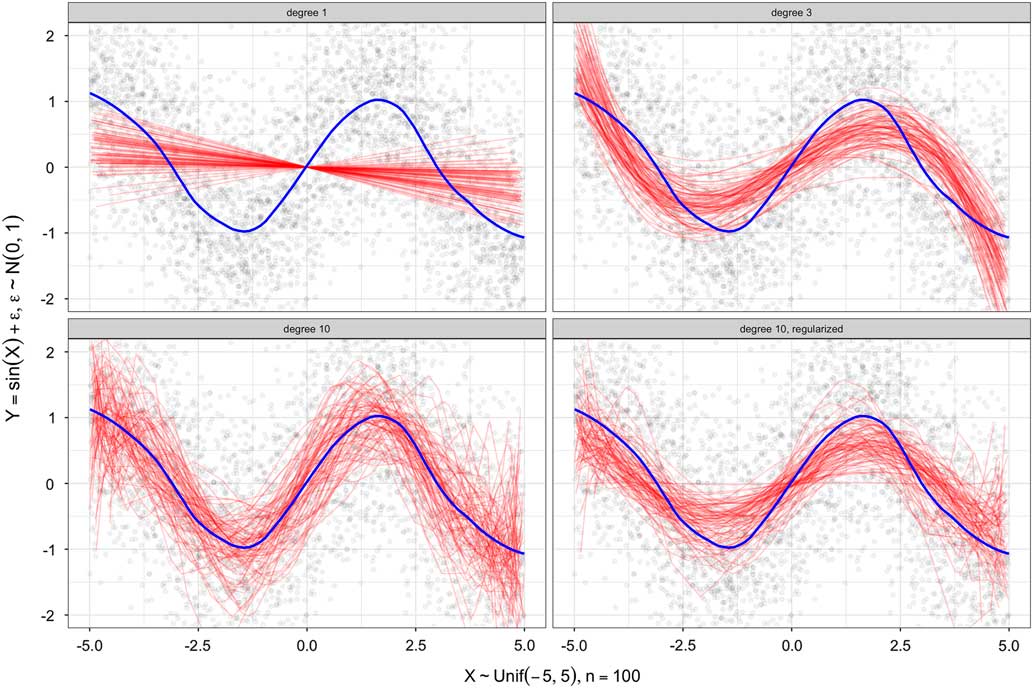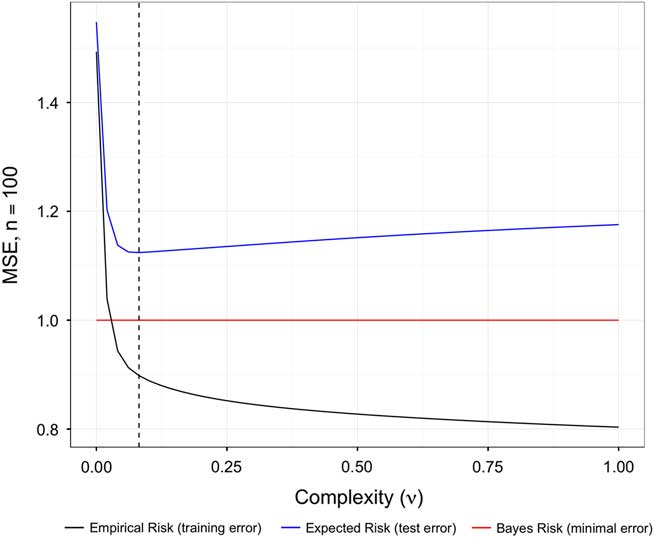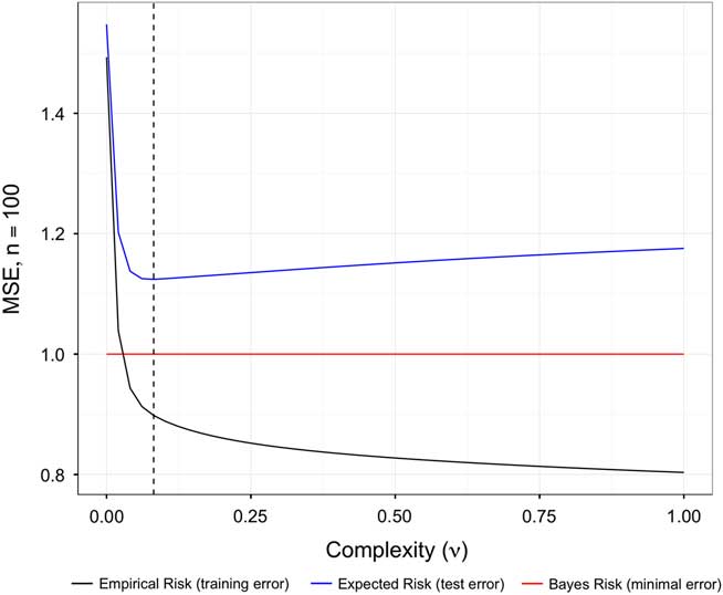This is the same as minimizing generalization error since the irreducible randomness in Y is assumed to have expectation 0. Figure 1 shows this tradeoff graphically with a simulated example (further details are shown in Table 1). Figure 2 gives another example of the bias–variance tradeoff in action with boosted regression.

Fig. 1

Here Y=sin(X)+є, where X~U(−5, 5) and $${\epsilon}\,\sim\,{\cal N}(0,1)$$ Note: The blue line shows the Monte Carlo estimate of $${\Bbb E}[Y\!\mid\!X\,{\equals}\,x]$$ across (x, y) drawn from the data-generating process. The red lines in each panel indicate the fit of the model to a particular sample. Each sample has 100 observations and the process is repeated 1000 times (75 randomly drawn examples shown in the figure). The linear case (fit by ordinary least squares) on the top left panel clearly underfits (the bias is high), though this estimator for f ^* has the lowest variance. The top-right panel shows a linear model with a degree 3 orthogonal polynomial expansion of x, which has much lower bias but a higher variance. The bottom left shows a linear model with a degree 10 orthogonal polynomial. The bias is smaller but the variance has increased relative to the top two panels due to overfitting. The model shown in the bottom right introduces a penalty term (a scalar λ) multiplied by the sum of the absolute values of the coefficients (the L ₁ norm of the coefficient vector), where λ is estimated by finding the value which minimizes an estimate of the generalization error using 10-fold cross-validation (Efron et al. Reference Efron, Hastie, Johnstone and Tibshirani2004; see also Kenkel and Signorino Reference Kenkel and Signorino2013 for a similar approach). This substantially reduces the variance of the predictions at the cost of a relatively small amount bias, producing a fit similar to that in the upper right. This fit has the smallest risk or generalization error. Table 1 gives further details.

Fig. 2

A learning curve for boosted regression trees (Hothorn et al. Reference Hothorn, Bühlmann, Kneib, Schmid and Hofner2010; Hothorn et al. Reference Hothorn, Hornik and Zeileis2014) Note: On the x-axis the complexity parameter ν is shown, increasing from left to right (higher is more complex). ν controls the “learning rate”: how quickly the model adapts to the data. On the y-axis the mean squared error of a series of fits to independent and identically distributed training data (n=100). Each fit is used to predict on the training set and the test set and is averaged over 1000 Monte Carlo iterations. At low levels of complexity, variance is low and bias is high: the expected and empirical risk is similar. As the complexity of the model increases, however, the difference between the empirical and expected risk diverges, with the former decreasing below the Bayes error rate (the theoretical minimum expected risk): overfitting the data. Minimizing the expected risk prevents overfitting that occurs when the empirical risk is minimized: the complexity parameter ν which minimizes the expected risk is denoted by the dashed vertical line (ν=0.08).

Table 1

Monte Carlo (1000 Samples) Estimates of the Expected Risk $$R(\hat{f})$$ , Empirical Risk $$\hat{R}_{n} (\hat{f})$$ , Excess Risk $R(\hat{f}){\minus}R(f^{{\asterisk}} )$ , and the Bayes Risk, R(f ^*) of Linear Models With Orthogonal Polynomials of Degree (1, 3, or 10), and a L ₁ Regularized Linear Model Fit to Training Samples of Length n=100 Drawn From Y=sin (X)+є Where $${\epsilon}\,\sim\,{\cal N}(0,1)$$ and X~U(−5, 5)

Note: The expected risk is minimized by the regularized linear model. Note also the divergence of the empirical risk and the expected risk as the degree of the polynomial increases. The regularized model is the most generalizable in this sense.

Flexible methods are desirable because they minimize bias, and simple methods are desirable because they have lower variance, both of which are components of excess risk. Regularization methods (e.g., the lower-right panel of Figure 1) penalize the complexity of a model in a manner that aims to minimize generalization error by making an optimal tradeoff between bias and variance: allowing a model to adapt to the data but not so much so that it overfits. Many of these regularization methods are heuristic, that is, they are not strictly optimal but they are computationally tractable. In the case of linear models, two popular forms of regularization are ridge regression and the least absolute shrinkage and selection operator (Lasso), both of which penalize regression coefficients using the size (norm) of the coefficient vector: the sum of the absolute values of the coefficients (the L ₁ norm), or the sum of the squares of the coefficients (the L ₂ norm) (61–73; Tibshirani Reference Vapnik1996; Hastie, Tibshirani and Friedman Reference Hastie and Tibshirani2009).Footnote ¹³ The function minimized when using ridge regression on a continuous outcome is shown below.Footnote ¹⁴

here y denotes a continuous real-valued outcome, p the number of predictors, β the regression coefficients, and n the number of observations which are assumed independent and centered by mean deviation (note that we omit an intercept for this reason, the empirical mean of y is 0). The only addition to the common least squares empirical risk function is the last term, where λ is a penalty parameter which is multiplied by the sum of the squares of each β _j . When this function is minimized at a particular value of λ, coefficients which are less useful in predicting y are shrunk toward 0. Thus, when this function is minimized, both the norm of the coefficient vector and the empirical risk are jointly minimized. This amounts to an application of Occam’s Razor: simpler solutions (i.e., smaller coefficient vector norms) are to be preferred, all else equal. That is, the coefficients are shrunk toward 0 if they do not contribute enough to the minimization of the empirical risk. How quickly shrinkage occurs is determined by the form of the penalty (e.g., the L ₁ or L ₂ norms of the coefficient vector) as well as the value of λ, which is usually selected to minimize generalization error (how this selection works is discussed further below). Parameter shrinkage makes regularized estimators less sensitive to the data (decreases their variance), which, again, can prevent overfitting.

The empirical risk function minimized when using the Lasso is similar and is shown below.Footnote ¹⁵ Note that the Lasso penalty may result in some elements of β being set of to (exactly) 0, unlike the ridge penalty.

The selection of how much to penalize the complexity of a model is an application specific problem which is usually solved by estimating generalization error at many values of the penalty parameter(s). This process which is often referred to as tuning or hyperparameter optimization. Though extensive discussion of this topic is beyond the scope of this paper, hyperparameter optimization is often much more sophisticated than an exhaustive search over a finite grid of tuning parameter values (grid search) and hence much more computationally efficient (see e.g., Bengio Reference Bengio2000; Bergstra and Bengio Reference Bergstra and Bengio2012). The expected risk of a model with a particular set of hyperparameters (in this case just λ) is often estimated using resampling methods. Then the value of the hyperparameter(s) which minimizes (or nearly minimizes) the resampled estimate of the generalization error is used. When data are independent and identically distributed we can use simple nonparametric resampling methods such as k-fold cross-validation or the bootstrap to estimate the generalization error of a model. Note also that regularization may be used with far more complex models, we discuss linear regression only because of its familiarity and simplicity.Footnote ¹⁶

Resampling methods work by treating the data at hand $${\cal D}_{n} $$ as the data-generating process $${\cal P}$$ , sampling from $${\cal D}_{n} $$ , and finding an estimate of f ^*, $$\hat{f}$$ , on each pseudo-sample. The bootstrap, for example, works by sampling n observations uniformly and with replacement from $${\cal D}_{n} $$ (Efron Reference Efron1982): analogous to simple random sampling from $${\cal P}$$ . $$\hat{f}$$ is estimated from this pseudo-sample and an estimate of the risk is obtained by computing the prediction error on the observations that are not in said psuedo-sample. k-Fold cross-validation is another common resampling estimator which divides $${\cal D}_{n} $$ into k randomly selected folds (groups of ${n \over k}$ observations sampled without replacement). $$\hat{f}$$ is learned on k−1 of the folds, and the risk is estimated by using $$\hat{f}$$ to predict on the kth held out fold. The procedure repeats so that each fold is held out from estimation of $$\hat{f}$$ , and the risk estimates from each iteration are averaged. Many variations on these two resampling methods are available (see e.g., Efron and Tibshirani Reference Efron and Tibshirani1994; Arlot et al. Reference Arlot and Celisse2010). Resampling methods are an active area of research, and these simple, well-known methods may not be the best choice in many situations (see e.g., Bischl et al. Reference Bischl, Mersmann, Trautmann and Weihs2012 for more recommendations).

Methods for dependent data are available but require additional assumptions about the dependence structure of the data-generating process and can be considerably more difficult to develop and use (Lahiri Reference Lahiri2003; Givens and Hoeting Reference Givens and Hoeting2012). For some sorts of dependent data, such as some types of time-series data, relatively simple nonparametric resampling methods are available (e.g., the moving block bootstrap). In other instances, Bayesian hierarchical models may be most effective (e.g., Tibshirani Reference Vapnik1996; Western Reference Wilcox, Sigleman and Cook1998; Gelman Reference Gelman2003; Gelman Reference Gelman2004; Park and Casella Reference Park and Casella2008). In other cases, bounds on generalization error can be estimated by using structural risk minimization (Vapnik Reference Wager and Athey1998). Discussion of structural risk minimization is beyond the scope of this paper but this appears to be a promising area of research with applications to social science data (see e.g., McDonald, Shalizi and Schervish Reference McDonald, Shalizi and Schervish2012 for recent work with macroeconomic data). In general the development of methods specific to political data may be a fruitful area of methodological research.

We emphasize that better estimates of generalization error will naturally result in a more optimally tuned model which will generalize better (in terms of prediction error). Hence, estimating generalization error and then adjusting the model to minimize this quantity is a means to maximize the predictive validity of a model’s predictions in situations where exact replication is not possible. We now turn to a discussion of how applied researchers might use our recommendations in future research.

Empirical Validation of Unspecified Functional Forms and Model Selection

It is often the case that the deductively valid theories used to specify models of empirical relationships in data are underdetermined.Footnote ¹⁷ What we mean by this is that the functional form that links outcomes and explanatory variables in an empirical model is usually not fully specified by the theory. We suggest that such models often do worse than they might have otherwise—in terms of predictive validity—had a more flexible functional form been selected.Footnote ¹⁸ Importantly, the use of predictive validity as a criterion for inference, another way of saying that there should be a focus on minimizing generalization error, provides a principled (in the sense that it increases predictive validity) way to use more flexible semiparametric and nonparametric models in observational and quasi-experimental research design settings. That is, it is possible to increase the predictive validity of a model by only constraining the empirical model in ways specified by the theory, and adopting a more flexible approach for other parts of the model. The use of regularized nonparametric or semiparametric methods (e.g., using methods such as boosting, generalized additive models, feedforward neural networks, kernel methods, or random forests, among many others) is often a much better option than an inflexible parametric model that is not fully implied by the theory.Footnote ¹⁹ Adopting a restrictive functional form where one is not directly implied is an arbitrary data analytic choice which impedes scientific progress by obscuring unexpected features of the data, which results in lower predictive validity.

Combining both a strict functional form deduced or encoded from a theory and a more flexible functional form to capture structure in the data where either the functional form is unclear or relevant measurements have not been obtained is an active area of research. Stage-wise methods such as boosting (e.g., “model-based boosting” and generalized additive models) offer well-developed implementations using well-studied statistical frameworks (Hastie and Tibshirani Reference Hastie, Tibshirani and Friedman1990; Friedman Reference Friedman2001; Hothorn et al. Reference Hothorn, Bühlmann, Kneib, Schmid and Hofner2010; Schapire and Freund Reference Schapire and Freund2012; Wood and Wood Reference Wood and Wood2015). It is also possible to combine more restrictive and more flexible functional forms by specifying latent variable models such as the latent space/factor class of models for networks (Hoff, Raftery and Handcock Reference Hoff, Raftery and Handcock2002; Hoff Reference Hoff2005; Handcock, Raftery and Tantrum Reference Handcock, Raftery and Tantrum2007; Hoff Reference Hoff2009). Ensembles of models estimated using different explanatory variables and combined by using a meta/super learner is also an attractive approach commonly referred to as stacking (Breiman Reference Breiman1996; LeBlanc and Tibshirani Reference LeBlanc and Tibshirani1996). Under certain conditions this approach also allows the estimation of sampling uncertainty (Sexton and Laake Reference Sexton and Laake2009; Mentch and Hooker Reference Mentch and Hooker2014; Wager, Hastie and Efron Reference Ward, Greenhill and Bakke2014). Another alternative approach is to not strictly specify any parts of the empirical model (i.e., only things like continuity or the maximal depth of interaction). Under this most flexible model, the hypothesized relationships can be compared with what the model learned from the data.

As we have argued above, generalization error can be used to make the optimal tradeoff between bias and variance. In the above discussion this has been “internal” in the sense that parameters of a model are found by the iterative minimization of estimates of generalization error. Generalization error can also be used for “external” model selection (Hastie, Tibshirani and Friedman Reference Hastie and Tibshirani2009; Arlot et al. Reference Arlot and Celisse2010). This would entail, for example, the comparison of models developed by different groups of researchers or that embodied different explanations for the process that generates outcomes. Absent a compelling alternative (such as a statistic which captures a particular type of structure in the data of theoretical importance), particularly in the cases we have focused on where the data-generating process is not under researcher control, preference for models with lower generalization error is arguably validity enhancing.Footnote ²⁰

We do not suggest that researchers adopt a single method, or even a particular class of methods in this paper; we simply wish to emphasize that researchers are likely selling their theories short in terms of predictive power by using overly restrictive models that are underdetermined by theory. We note that, though most examples are relatively new, the call for more focus on predictive checking is not new to applied political science research (see e.g., Beck, King and Zeng Reference Beck and Jackman2000; Ward, Greenhill and Bakke Reference Western2010; Beger, Dorff and Ward Reference Beger, Dorff and Ward2014; Hill and Jones Reference Hill and Jones2014; Schnakenberg and Fariss Reference Fariss2014; Chenoweth and Ulfelder Reference Chenoweth and Ulfelder2015; Douglass Reference Douglass2015; Graham, Gartzke and Fariss Reference Graham, Gartzke and Fariss2015). Given the importance of predictive checking, and the recent discussion of transparency and the replication standard—we view exact replication as specifically a form of model validation—it is an important point to re-emphasize here: regularizationFootnote ²¹ can be used to decrease threats to predictive validity from over/underfitting an empirical model by focusing on the minimization of generalization error.Footnote ²² Moreover, “data mining” (i.e., the use of statistical/machine learning techniques), when used in the principled fashion described here, should not be used as a pejorative term. Instead, such tools should be adopted to help provide evidence for the predictive validity of observational and quasi-experimental designs when exact replication is not possible.