1 Introduction
Quantitative temporal constraints are essential for many real-life planning and scheduling domains (Smith et al., Reference Smith, Frank and Jónsson2000). Many systems adopt a Simple Temporal Network (STN; Dechter et al., Reference Dechter, Meiri and Pearl1991) to represent and reason over the temporal aspects of such problems, associating time points with the start and end of actions, and modelling the temporal relations by binary simple temporal constraints. We present a general, efficient message-passing scheme for propagation of such constraints, and evaluate its insights for semi-structured networks that arise in Hierarchical Task Network (HTN) planning systems. This paper extends the preliminary report of our work (Bui et al., Reference Bui, Tyson and Yorke-Smith2007, Reference Bui, Tyson and Yorke-Smith2008).
The central role of STNs in deployed planning systems (Laborie & Ghallab, Reference Laborie and Ghallab1995; Myers et al., Reference Myers, Tyson, Wolverton, Jarvis, Lee and desJardins2002; Bresina et al., Reference Bresina, Jónsson, Morris and Rajan2005; Castillo et al., Reference Castillo, Fdez-Olivares and García-Pérez2006) makes efficient inference with STNs especially important. The two principal inference tasks, determining consistency of an STN and deriving its minimal network, can be achieved by enforcing path consistency (PC; Dechter et al., Reference Dechter, Meiri and Pearl1991). The common approach is to run an All-Pair Shortest Path graph algorithm on the distance graph of the STN. Algorithms such as Floyd–Warshall (denoted F-W or PC-1; time complexity Θ(N 3)), or Johnson (complexity Θ(N 2 log N + NM, where M is the number of edges in the constraint graph) can be used (Cormen et al., Reference Cormen, Leiserson and Rivest1990).
To achieve better efficiency, significant efforts have been made to apply more sophisticated constraint propagation techniques to STNs. Partial Path Consistency (PPC; Bliek & Sam-Haroud, Reference Bliek and Sam-Haroud1999) can be applied to a triangulated (or chordal; Kjaerulff, Reference Kjaerulff1990) constraint graph rather than a complete graph and is sufficient for backtrack-free reconstruction of all solutions. Until recently, the state of the art, ΔSTP (Xu & Choueiry, Reference Xu and Choueiry2003), is a specialized solver based on PPC and operates over triangles of the triangulated STN. If only consistency is required, but not the minimal network, Directional Path Consistency (DPC) can be used with time complexity  , where w is the induced tree width along the node ordering used (Dechter, Reference Dechter2003).
Empirical comparisons on random STNs (Xu & Choueiry, Reference Xu and Choueiry2003; Shi et al., Reference Shi, Lal and Choueiry2004) show that ΔSTP outperforms PC-1, Johnson’s Algorithm (‘Bellman-Ford’), and is comparable to (on dense graphs) or outperforms (on sparse graphs) DPC. Although the worst-case time complexity of ΔSTP, unstated in (Xu & Choueiry, Reference Xu and Choueiry2003), is not known, instances have been constructed where ΔSTP processes as many as a quadratic number of triangles (Planken et al., Reference Planken, de Weerdt and van der Krogt2008). The number of triangles of the triangulated STN is bounded above by  ; the bound is attained for a complete graph.
Despite the variety of methods, no dedicated STN solver takes full advantage of the tree decomposition of the STN constraint graph, namely, the ability to decompose a constraint graph into a ‘tree’ of variable and constraint clusters (Dechter & Pearl, Reference Dechter and Pearl1989). One exception is the specialized solver SR-PC (Yorke-Smith, Reference Yorke-Smith2005) that exploits the structure of STNs associated with plans in the HTN planning paradigm (Erol et al., Reference Erol, Hendler and Nau1994). The HTN planning process gives rise to STNs with the sibling-restricted (SR) property. Such an SR-STN can be decomposed into a tree of smaller sub-STNs, mirroring the shape of the hierarchical structure in the plan. SR-PC traverses this tree, invoking an STN solver at each sub-STN. While SR-PC shows strong empirical performance on SR-STNs, it does not operate on general networks.
In contrast to STNs, tree-decomposition methods are often applied to the general Constraint Satisfaction Problem (CSP). These methods, such as variable elimination (adaptive consistency) and cluster tree elimination (CTE; Dechter, Reference Dechter2003), operate by decomposing a triangulated constraint graph into a tree of variable clusters and solving the subproblem in each. Sophisticated decomposition-based methods for the (discrete) CSP (e.g. Jégou & Terrioux, Reference Jégou and Terrioux2003) have enjoyed success on appropriate problems (e.g. Larrosa et al., Reference Larrosa, Morancho and Niso2005); they can be seen as specializations of CTE and other generic variable elimination methods.
In this paper, we apply the ideas of such tree-decomposition methods to the STN. Note that a direct application of tree-decomposition methods to the STN is non-trivial. Since the STN represents a CSP with continuous variables, it is not clear how to represent the ‘messages’, that is, the sets of additional constraints resulting from eliminating some variables. We first show that, for an STN, these messages can be represented compactly as sub-STNs. We then present an efficient message-passing scheme, called Prop-STP. Like ΔSTP, Prop-STP requires the STN to be triangulated; however, unlike ΔSTP, Prop-STP operates over the set of maximal cliques of the triangulated constraint graph. The time complexity of Prop-STP is  where K is the number of cliques, and w is the induced tree width (the size of the largest clique minus 1). For STNs with known and bounded tree width (e.g. SR-STNs), Prop-STP thus achieves linear time complexity, a substantial improvement over the use of All-Pair Shortest Path algorithms. Empirically, Prop-STP achieves the same level of performance on structured SR-STNs as the specialized solver SR-PC.
Subsequent to our work, but independently, Planken et al. (2008) have introduced P3C. Like ΔSTP, P3C operates on the triangulated STN. Akin to how ΔSTP is a dedicated implementation of PPC on the network, so P3C is an implementation of DPC but with an additional phase. This second phase ensures that the minimal network is derived. P3C has provable linear worst-case complexity in the number of triangles. Although in practice the worst-case behaviour of ΔSTP does not arise, empirical results reveal a performance edge for P3C on several benchmark network types.
Triangulation of an STN can be carried out efficiently by greedy methods (Kjaerulff, Reference Kjaerulff1990). Empirical results demonstrate that, even with a triangulation step, ΔSTP and P3C outperform earlier STN solvers (Xu & Choueiry, Reference Xu and Choueiry2003; Shi et al., Reference Shi, Lal and Choueiry2004; Planken et al., Reference Planken, de Weerdt and van der Krogt2008). Our analysis of Prop-STP offers an insight into how to order the triangles in ΔSTP, and also shows that ΔSTP’s complexity can be characterized in terms of the induced tree width. We further provide a new perspective on P3C from the viewpoint of variable elimination. Experiments with semi-structured STNs of limited tree width indicate that Prop-STP performs at least comparably with ΔSTP even when provided with no information about the STN structure. This indicates that it is more efficient to operate on cliques rather than on triangles, as anticipated by (Choueiry & Wilson, Reference Choueiry and Wilson2006).
2 Background and terminology
We begin with the background necessary for the message-passing scheme for STNs and the resulting Prop-STP algorithm. We are concerned with the relationship among a set of variables {xi, i∈S}, each taking values from the domain
 . A relation
 over S is simply a subset
 . The index set S is called the scope of
 . We make use of two standard relational operators: projection and join. Denote the projection of a relation
 onto the index set
 by πV
 , and the join of
 and
 by
 .
2.1 Simple temporal networks
An STN is represented by a set of variables {xi|i∈S}, representing time points, with domain  Footnote 1; a set of interval unary constraints
 , where
 ; and a set of binary constraints
 , i < j where
 Footnote 2. Generally, we assume that there are N variables, so S = {1,…,N}. Given an STN
 , its constraint graph G is an undirected graph with vertices representing the variables; an edge links xi and xj iff the binary constraint
 exists.
We differentiate the constraints represented by  and the relation they imply, denoted by
 and called the solution set of the STN. By definition,
 is a relation with scope S that is the join of all the unary and binary constraints
 and
 . Thus, every solution in
 is an assignment of values to time points such that all constraints are satisfied. Relational operators such as join and projection can be applied on the solution set with the usual set semantics. An STN is consistent iff its solution set is non-empty. Two STNs are equivalent (denoted by
 ) iff their solution sets are the same, while two STNs are equal (denoted by
 ) iff they contain exactly the same set of constraints.
We introduce some useful operators that operate directly on  . Let V be a subset of the variables. The subnetwork of
 restricted to V, denoted by
 , is the STN with scope V and constraints
 for i, j∈V. Any solution of
 of course will satisfy the constraints of
 , so
 . When
 , that is when
 faithfully represents the set of feasible assignments to V given the constraints in
 , the STN is said to be locally minimal on V. We next consider two STNs
 ,
 with different scopes S 1, S 2 and constraint graphs G 1, G 2, respectively. The join of
 and
 , denoted by
 , is the STN with scope S 1∪S 2 and constraint graph being the superimposition of G 1 and G 2. All constraints in G 1 (but not in G 2) and in G 2 (but not in G 1) are taken from
 and
 , respectively, and all constraints in both G 1 and G 2 are the pairwise intersection between constraints of
 and
 . Intuitively,
 is obtained by merging two set of constraints from
 and
 . It is straightforward to show that
 .
An STN  has an equivalent minimal network representation
 whose constraints satisfy
 , and
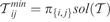 for all i < j. Hence,
 is locally minimal on {i} for all i, and on {i, j} for all pairs (i, j). The constraint graph of
 is thus a complete graph. The operation to find the minimal network (producing
 given
 ) is called minimalization and is the principal inference task for STNs.
It has been shown that STNs are binary decomposable (Dechter et al., Reference Dechter, Meiri and Pearl1991), that is, for every subset of variables V, the projection  is expressible as a binary constraint network. Further still, the minimal network of
 is precisely
 , the minimal network of
 , restricted to V Footnote 3. Thus, for every V

A weaker notion, the partial minimal network, is denoted by  and defined by the set of constraints
 , and
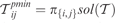 for all i < j and (i, j) ∈ edges(G). The partial minimal network thus shares the same constraint graph G with the original network, and can be obtained from the minimal network
 by removing all binary constraints on edges that are not present in G. If the constraint graph of
 is triangulated, given
 , every solution to
 can be constructed backtrack-free.
2.2 Variable and CTE
Complementary to methods that solve a CSP based on the iteration of narrowing operators, such as PC-1 and ΔSTP (which can be seen as AC-3 operating over triangles Xu & Choueiry, Reference Xu and Choueiry2003), an alternative method for the general CSP is called adaptive consistency or variable elimination (Dechter, Reference Dechter2003). Given a general (binary) CSP  with scope S, consider two sets of variables (called clusters), W and V, that together cover the constraint graph G (this means W∪V = S and every edge in G belongs entirely in W or in V). If every path between W and V in G passes through W∩V, we say that the two clusters are separated by their separator W∩V, denoted by sep(W,V). It is then possible to project onto W:

where  is the message from V to W. This operation effectively ‘eliminates’ all variables in V − W. By eliminating the variables in a given order, we can obtain the minimal constraints. The complexity of this method thus hinges on the representation and the calculation of the messages. Owing to the difficulty in representing the messages for variables with a continuous domain, this idea has not been applied to STNs whose domains are inherently continuous (Dechter, Reference Dechter2003: 357).Footnote 4
CTE is a generalized variable elimination method for computing the partial minimal network  for a triangulated constraint graph (Dechter, Reference Dechter2003). The algorithm works by decomposing the triangulated graph G into a join tree (or a junction tree) over a set of variable clusters {V 1,…,VK} that cover the original graph G. The vertices V 1,…,VK of a join tree have the property that, for every tuple (i, j, k) s.t., j lies on the path between (i, k), Vi∩Vk
 Vj. Once a join tree is constructed, messages can be passed asynchronously among the clusters along its edges. After a message has been passed in each direction on every edge of the join tree, the resulting network can be shown to be locally minimal on every cluster Vi. Solving the local networks at each cluster then yields all the minimal constraints needed for the partial minimal network.
3 STN propagation: Prop-STP
In this section, we discuss in detail how the main idea in the variable and CTE can be made to work efficiently with STNs. We first show how variable elimination and message passing in CTE can be implemented via standard STN operations. We then present Prop-STP, a new STN solver based on an improved propagation scheme for STNs, and develop a formal proof of its correctness. Detailed analysis of the new algorithm and discussion in the context of other STN solvers are also provided.
3.1 Variable elimination for STNs
We now focus on the STN. First observe that since every STN is binary decomposable, its projection onto an arbitrary subset of variables can be computed and represented by the minimal network (Equation (2.1)). Applying this to the calculation of the message in variable elimination yields

The message thus can be represented compactly and conveniently as the STN  , which is simply the minimal network of
 , restricted to the separator set. We call this the message STN, denoted by μ(V,W). Using this compact representation of the messages, we immediately obtain an efficient variable elimination procedure.
Theorem 1. Consider an STN  and let V,W be two clusters of variables that cover the constraint graph G. Suppose that V and W are separated by sep(V,W) = V∩W. Then the projection of
 onto W,
 , can be represented by the solution of the STN

Proof. Substitute (3.1) into (2.2) and use  .□
The above expression involves only a minimalization operation on  and a simple restriction to the separator set. Any of the STN solvers described earlier that produces the minimal network can be used for the former operation. (PPC-based methods such as ΔSTP and DPC-based methods such as P3C can be used. However, the subgraph in the separator must be complete, and the subgraph in V must be triangulated.) Since minimalization creates a complete graph, the constraint graph of the STN
 is a complete graph over sep(V,W). Hence, unless
 is also complete over sep(V,W), the operation in (3.2) will introduce new edges to the original constraint graph of
 .
3.2 Message passing for STNs
Once we have a compact representation of the messages, the CTE algorithm can be applied immediately to compute the partial minimal network  . Let us assume that we are given a join tree
 over a set of clusters V 1,…,VK that cover the original constraint graph G. In some cases, such a join tree can be found from the structure of G, as in the case of SR STNs, or it can be found by first triangulating G and then extracting the set of maximal cliques of the resulting triangulated graph.
The standard message-passing scheme used in CTE (Dechter, Reference Dechter2003) computes a message from a cluster Vi to a neighbouring cluster Vj, using the messages Vi received from its other neighbours. Representing the message from Vi to Vj by the message STN μ i, j, we obtain
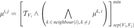
To compute each message requires a minimalization operation over one cluster. After computing all such messages, we must go through each cluster and minimalize it (with the neighbour messages included). Since there are 2(K − 1) messages, the total is 2(K − 1) + K = 3K − 2 minimalization operations. We obtain the minimal domain  for all i, but only
 for those (i,j) that belong to the same cluster. Since any edge in G must belong to one of the clusters, we obtain the partial minimal network.
3.3 An improved propagation scheme
We can exploit specific properties of STN to make the message-passing scheme more efficient. In the above, one minimalization operation is needed for each message. However, binary decomposability of STNs implies that all possible projections of  onto an arbitrary subset of its variables can be computed in a single minimalization operation. Thus, we can rearrange the order of message passing so that one minimalization operation can compute multiple messages. Furthermore, as we show below, it is possible to eliminate the need to store the messages all together.
Given the join tree  , a cluster ordering V 1,…,VK is termed valid if whenever Vj lies on the path from Vi to VK, then j ⩾ i. Such a valid ordering can easily be created by choosing an arbitrary cluster to be VK and treating it as the root of
 . A valid cluster ordering then places earlier the clusters that are further away from the root.
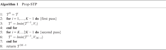
The atomic building block of the algorithm that we propose (see Algorithm 1) is a simple operation on STNs, termed local minimalization, which takes a subnetwork and replaces it with its minimal network. Given a subset of variables V, a local minimalization on V returns the STN  . Since
 , it is trivial to see
 (since, if T 1 is a sub-STP of T 2, then
 ). Note that this operation makes the constraint subgraph in V complete.
Let  . The next two lemmas identify important properties of the lmin operation, which will be used in the main proof of correctness of our algorithm.
Lemma 2.If  is locally minimal on some
 then so is
 .
Proof. Observe that  constraints are tighter, so
 . Therefore, if
 then we must have equality, which implies
 is also locally minimal on W. □
Lemma 3. For any P  V such that P separates V − P and
 ,
 is locally minimal on
 .
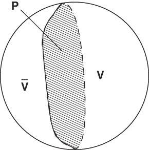
Proof. For an illustration of the sets V,  and P, see Figure 1. Let
 , so that P = sep(V,W). Now by Theorem 1,
 . In this equality, the LHS is the same as
 . In the RHS
 is the same as
 . Thus,
 , hence
 is locally minimal on W.□
Illustration of the separator set P

Note that as long as we can find a separator P that is a proper subset of V, then  is a proper subset of S. Thus, while the original STN
 is (of course) locally minimal on S, the new STN
 is locally minimal on a proper subset of S. By repeatedly applying the same kind of operation, we can obtain the minimal constraints. This is the basic idea of our algorithm, which we call Prop-STP; pseudo-code is shown in Algorithm 1.
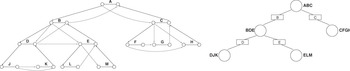
Example:Figure 2 depicts an STN arising from a hierarchical planning problem. The edges labelled with letters refer to tasks; each models the duration between the start and end time points of that task. For example, letter A refers to two time points (variables) Astart and Aend. The other edges model precedence constraints between parent and child tasks, together with a representative sample of other temporal constraints. The STN has the SR property, which provides a simple clustering of the variables to yield the join tree  shown on the right. The separators of each cluster are depicted in the rectangular boxes. On this STN, the first pass of Algorithm 1 processes the clusters in an order such as DJK, ELM, BDE, CFGH, and ABC. Hence, the cluster ABC is the root of the join tree. The second pass processes CFGH, BDE, ELM, and DJK. A single lmin operation on BDE in the second pass effectively computes the two messages to DJK and ELM at once. At the end, we obtain the minimal subnetwork for each cluster, and thus the partial minimal network for the whole STN.
Left: STN; right: join tree of clusters

We now provide a formal proof that this algorithm returns all the minimal constraints of the original network.
Theorem 4. At the end of Prop-STP,  is locally minimal on every cluster Vk; furthermore, the subnetwork
 is a minimal network. As a result,
 is locally minimal on every variable i, and on every pair of variables {i,j} for all (i,j) belonging to the same cluster.
Proof. We proceed by induction on the number of clusters K in the join tree. The base case is trivial, so assume the theorem holds for any join tree with K − 1 clusters.
Let  . Since V 1 must be a leaf node in
 , if we let
 then P separates V 1 − P from
 . Thus, by Lemma 3,
 is locally minimal on
 .
Let  be the subnetwork of
 over S 1 and
 be the join tree
 minus the cluster V 1. Observe that
 has K − 1 clusters and that the ordering V 2,…,VK is a valid one for
 . Running Prop-STP on
 would produce the STN
 . Applying the inductive hypothesis, we observe that
 is locally minimal on all Vi, i ⩾ 2, as well as on every variable and pair of variables contained within these clusters. Observe that
 is locally minimal on S 1 (since
 is, and using Lemma 2), so the projection of
 onto Vi (i ⩾ 2) is the same as the projection of
 . It follows that
 itself is locally minimal on all Vi, i ⩾ 2, and on all variables and pairs of variables within these clusters, and so is
 (Lemma 2).
It remains to be shown that  is also locally minimal on V 1 and that the subnetwork
 is a minimal network. By Theorem 1,
 is the solution of the STN
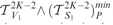 . Examining the separator P, we see that it must be a subset of some Vi, i ⩾ 2, so the reasoning in the previous paragraph implies that the subnetwork
 is already minimal; that is,
 . Thus,
 is the solution of the STN
 . Therefore,
 is locally minimal on V 1, and so is
 . Finally, the last lmin operation is invoked on V 1, so afterwards
 is locally minimal on every variable and pair of variables in V 1.□
3.4 Analysis of the new algorithm
Instantiations of Prop-STP can be implemented using different STN subsolvers to perform the lmin operation. For example, using PC-1 (Floyd–Warshall) leads to Prop-PC1-STP. Since there are precisely 2K − 1 lmin operations, each with complexity  , the overall complexity of Prop-PC1-STP is
 . An improvement can be made by keeping track of which clusters have not been changed after the lmin operations in the first pass, so that in the second pass we need not perform lmin on them again.
Since Prop-STP effectively completes the constraint graph within each cluster Vi, the resulting global constraint graph is triangulated. In practice, one can triangulate G in the initialization phase; if so, the constraint graph is already complete within each cluster. In this case, Prop-STP returns the partial minimal network  of the triangulated G. Like other algorithms that work on triangulated graphs, such as PPC and ΔSTP, Prop-STP does not return the full minimal network. However,
 is sufficient for a triangulated graph since every solution can be constructed backtrack-free from the partial minimal network.
It is interesting to examine the behaviour of our algorithm when we use ΔSTP as the subsolver at each cluster (although this is not likely to result in a performance improvement since the subgraph at each cluster is already complete). In this case, Prop-Δ-STP will process triangles in G, one by one, but following the order imposed by our propagation scheme: all triangles within each cluster are processed until stabilized before moving on to triangles in another cluster. As noted by (Xu & Choueiry, Reference Xu and Choueiry2003), the order in which triangles are processed has a crucial effect on the performance of ΔSTP. The improved order of triangle processing in our algorithm also agrees with the intuition of the authors of the ΔSTP algorithm and others (Choueiry & Wilson, Reference Choueiry and Wilson2006).
We also provide an explanation for the behaviour of P3C. The latter is motivated from DPC, building on the ideas of ΔSTP. Supposing a general triangulated STN, algorithms Prop-STP and P3C perform essentially the same computation of two passes, if given the same vertex ordering. The first pass of P3C, achieved by enforcing DPC, can now be seen as the forward passing of messages; the second pass, achieved by explicit propagation over triangles, is the return of messages from the root. Prop-STP does compute the join tree, whereas P3C works directly on the triangles, and Prop-STP can incur further overhead compared to P3C by considering some triangles more than strictly necessary (those in the intersection of clusters). However, this in turn allows Prop-STP to operate over untriangulated networks for which the cluster decomposition is known.
4 Experimental results
We undertook experiments to investigate the behaviour of Prop-STP. We investigate the performance as the structure and size of the STN vary, and we compare Prop-STP against the existing STN solvers SR-PC and ΔSTP to gain insight into their relative strengths. Since Prop-STP is designed to leverage structure in the network, in the form of a tree decomposition, we develop benchmarks based on structured STNs arising from HTN plans.
4.1 Sibling-restricted STNs
HTN planning assumes a hierarchical flow, with high-level tasks being decomposed progressively into collections of lower-level tasks through the application of matching methods with satisfied preconditions. In an SR STN, constraints may occur only between parent tasks and their children, and between sibling tasks. This restriction on what STN constraints may exist between plan elements is inherent to HTN planning models; in particular, there is no way in standard HTN representations to specify temporal constraints between tasks in different task networks (Erol et al., Reference Erol, Hendler and Nau1994). The specialized STN solver SR-PC (Yorke-Smith, Reference Yorke-Smith2005) transverses a tree of sub-STNs that correspond to the decompositions in the HTN plan. Since the STNs thus considered are small, compared to the global STN corresponding to the whole plan, the overall amount of work to enforce PC is much less.
Despite its success on benchmark problems from the PASSAT plan authoring system (Myers et al., Reference Myers, Tyson, Wolverton, Jarvis, Lee and desJardins2002), SR-PC has two drawbacks. First, standard HTN representations have been extended to support limited coordination between different task networks via landmark variables (Castillo et al., Reference Castillo, Fdez-Olivares and García-Pérez2006) that allow synchronization of key events in the plan. SR-PC can accommodate, though awkwardly, a small number of such landmark variables and their corresponding constraints. Second, although not exhibited in practice, SR-PC has a poor and weakly characterized worst-case theoretical complexity.
The small tree width w of an SR network means that Prop-STP will be particularly efficient for this class of STNs, provided we can find an optimal or near-optimal decomposition of the constraint graph G of the global STN into a join tree, and a cluster ordering over this tree. Fortunately, there is a natural decomposition based on each parent task T and its children Ti. Specifically, we form into a cluster the start and end time point variables of task T and all its Ti, and all temporal relations between them (including those between the children). Figure 2 illustrates this clustering. Since task networks typically comprise a handful of tasks, the size of each cluster is small. Therefore, performing minimalization on each cluster, as done in Prop-STP, is anticipated to be much more efficient than computing the minimal network for the global STN. In general, if we consider a task network represented by a balanced tree with depth d and branching factor f (hence, the number of nodes is  ), the complexity of Prop-STP is
 (the join tree has
 clusters, each with size
 ).
We also note that an SR STN has no articulation points. Since each task in the HTN corresponds to two variables, as can be seen in Figure 2, the constraint graph is biconnected and decomposes only via separator sets of cardinality at least twice. This hampers algorithms that seek articulation points, whether explicitly, such as F − W + AP, or implicitly, such as ΔSTP. Observe that Prop-STP can work on the untriangulated constraint graph with this clustering. To apply a generic STN solver such as ΔSTP or P3C in this case requires triangulation of the whole constraint graph G, which in general introduces many more new edges than the total in all the completed G (i) combined.
4.2 Experiments with semi-structured STNs
To validate the concept of Prop-STP, we implemented the algorithm within the PASSAT HTN plan authoring system. Our first Prop-STP implementation was written in Lisp to allow a fair comparison with the existing Lisp-based implementations of SR-PC and ΔSTP, and to allow integration with the PASSAT system. However, as reported in the preliminary results in (Bui et al., Reference Bui, Tyson and Yorke-Smith2007), this implementation of the three algorithms suffered from excessive CPU runtimes, an artefact, due to the simplistic memory handling of our Lisp environment. Hence, we developed a second implementation of the algorithms in Java; direct integration with PASSAT was not attempted.
The benchmark networks we employed were created by a generator that yields STNs akin to those produced by PASSAT, from random plans with a uniform tree of tasks, as described in (Yorke-Smith, Reference Yorke-Smith2005). The generation parameters include plan size (specified by HTN depth and mean branching factor), constraint likelihood, constraint tightness, ratio of time points that are landmarks, and STN consistency.
The experiments were conducted on a 2 GHz Pentium M with 2GB RAM, using Java 1.6. A timeout of 10 minute was enforced. Unless stated, the results average 50 runs, and error bars depict 95% confidence intervals.
The algorithms we report are PC-1 as a baseline, ΔSTP (with and without triangulation time), and Prop-STP. ΔSTP source code was kindly made available by its authors. When the landmark ratio is 0, the STN is SR, and SR-PC can be applied. We verified that Prop-STP behaves as SR-PC in this case, when given the decomposition of the network; its runtime and constraint checks equal those of SR-PC.
We gave the same networks to ΔSTP and Prop-STP, and did not provide any additional information about structure to Prop-STP. Information about the STN’s construction from the HTN structure and landmark variables would enable decomposition with the addition of a minimal number of triangulation fill and cluster completion edges. Prop-STP would benefit from this information (which is not pertinent to ΔSTP); thus, we held back Prop-STP from its full potential. This decision allows us to compare Prop-STP in the ‘worst case’ and assess its behaviour on STNs where the structure is not known a priori. Throughout, the same triangulation heuristics are used for all algorithms.
We experimented with two variants of Prop-STP, one using PC-1 and the other using ΔSTP as the STN subsolver. Recall that in Algorithm. 1, the subgraph at each cluster is a complete clique, and that such dense graphs are those most favourable to PC-1 (Shi et al., Reference Shi, Lal and Choueiry2004).
We recorded two metrics: first, the total CPU runtime in milliseconds for each algorithm variant (the recorded time for Prop-STP’s ‘no triangulation’ variant still includes the time to complete each cluster), and second, the counted number of constraint checks.
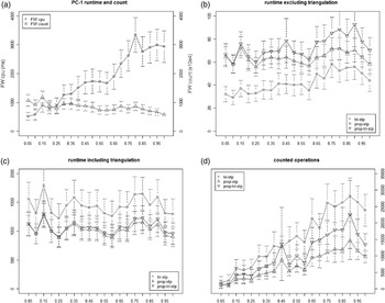
Consistency:Figure 3 varies the consistency of the generated STN from 5% to 100%, for problems of mean depth 5 and mean branching factor 3.5 (approximately 500 nodes), and a landmark ratio of 5%. Note that the y axis scale varies between the graphs. PC-1 is most sensitive to the consistency of the network, taking considerably longer for consistent than for inconsistent STNs but, curiously, performing fewer constraint checks for the former. There is little to distinguish between ΔSTP, Prop-PC1-STP, and Prop-Δ-STP in terms of runtime when triangulation time is excluded; when included, ΔSTP is slightly slower. In terms of counted operations, all three perform more constraint checks for consistent STNs. ΔSTP is most sensitive to consistency, Prop-PC1-STP the least, and Prop-Δ-STP blends the two, as could be expected.
Landmark STNs, as consistency varies

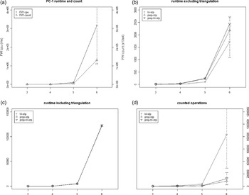
Problem size:Figure 4 varies STN size, in terms of underlying plan depth, from 3 to 6; consistency is 50%, landmark ratio is 5%, and mean branching factor is 4. The size of the STN grows exponentially with depth. An algorithm that scales linearly with problem size will therefore scale exponentially with depth. Figure 4 includes data only for those instances for which every algorithm succeeded; we exclude data for depths 7 and 8, where often only Prop-STP succeeded. PC-1 and ΔSTP, respectively, suffer from timeout or memory exhaustion.Footnote 5 Prop-STP solves these instances, continuing to exhibit the same scaling behaviour as in the figure. As expected, even in the data presented, we see that all algorithms increase exponentially with depth, that is, polynomially in problem size. As in Figure 3, we observe that the runtime metrics for ΔSTP and Prop-STP are similar, while ΔSTP employs more constraint checks.
Landmark STNs, as depth varies

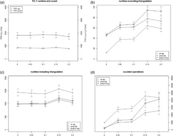
Structure:Figure 5 varies the landmark ratio from 0% to 20%, for problems of depth 5 and consistency of 50%. A low value for landmark ratio corresponds to a structured (more SR-like) STN; a higher value corresponds to a more unstructured STN, closer to a general random network. A value even of 10% leads to a very dense network after triangulation.
Landmark STNs, as landmark ratio varies

While PC-1 is largely insensitive to the landmark ratio parameter (network consistency being more significant), ΔSTP and Prop-STP exhibit greater runtime as structure decreases. Most clearly, this is seen in runtime excluding triangulation and in counted operation: the triangulation time masks the underlying computational effort. The reason that Prop-STP does not perform significantly better than ΔSTP lies in our giving it no information about network structure. As observed earlier, Prop-Δ-STP (in particular) explains the theoretical performance of ΔSTP with optimal triangle ordering. Since we apply both methods to the same triangulated graph with the same heuristics, we should expect to observe a similar performance in practice in this case.
5 Discussion
The picture that emerges for semi-structured STNs is that Prop-STP performs comparably with the state-of-the-art solver ΔSTP. The empirical findings confirm that it scales polynomially with problem size. The more structured the network, the better the relative performance, and better still if Prop-STP is informed about network structure, as in the experiments reported in (Bui et al., Reference Bui, Tyson and Yorke-Smith2007) for SR-STNs. Given no structure, Prop-STP performs best on sparse networks, since a tree decomposition is more amenable in general the fewer the edges in the triangulated graph. Empirically, on our benchmark semi-structured STNs, the join tree uncovered has an average cluster size approximately equal to the 1 + branchingfactor. Approximately described, the behaviour of Prop-Δ-STP exhibits characteristics of the two solvers from which it is composed.
We have not directly compared Prop-STP and P3C. Such an empirical comparison holds little interest, since the two (although originating from different motivations) perform essentially the same computation, supposing the same triangulation and vertex ordering. The results of (Planken et al., Reference Planken, de Weerdt and van der Krogt2008) show a performance edge for P3C over ΔSTP, thus confirming our results for Prop-STP over ΔSTP.
It is worth noting that our implementation of Prop-STP contains no effort to optimize the network decomposition, nor leverage reuse of, for example, triangulated clusters. The benefit of the set of smaller subproblems that Prop-STP tackles comes at the cost of computing the decomposition into clusters and exchanging the messages between them; the number and size of the separator sets are key. A carefully engineered implementation can be expected to reduce the runtime by a constant factor. Thus, the pattern for relative CPU times reported above can be expected to match the pattern for counted operations: a modest runtime advantage including triangulation time for Prop-STP over ΔSTP provided that the network has sufficient structure (i.e. landmark ratio is small). This is true even though we provide no structural information to Prop-STP.
The tree decomposition and clustering that benefit Prop-STP on sparse and structured networks are expected to hinder it on dense and unstructured networks. For completeness, we experimented on general STNs, randomly created by the generator of (Xu & Choueiry, Reference Xu and Choueiry2003). The results, not reported here, indeed suggest that the computational overhead of Prop-STP puts it at a disadvantage compared to ΔSTP in terms of runtime. In this case, P3C is preferable because it sidesteps computation of the join tree. We also confirm the results in the literature that ΔSTP is most effective for sparse networks (Shi et al., Reference Shi, Lal and Choueiry2004). As in the case of structured networks, we find that Prop-PC1-STP is relatively insensitive to the constrainedness, while the behaviour of Prop-Δ-STP is again a blend of the two solvers from which it is composed.
6 Conclusion and future work
We consider a new method, Prop-STP, for solving Simple Temporal Networks in the case of continuous as well as discrete variable domains. In contrast to methods based on graph algorithms or on iteration of narrowing operators, our algorithm is based on an efficient message-passing scheme over the join tree of the network. The complexity of Prop-STP depends on the minimalization operator, that is, the STN solver used to enforce PC on subproblems. Thus, consistency and the minimal constraints of an STN (from which solutions can be derived backtrack-free) can be determined with complexity  or better, where K is the number of cliques and w is the induced tree width. For STNs with known and bounded tree width, Prop-STP thus achieves linear time complexity. The new propagation scheme provides formal explanation of the performance of the existing STN solvers ΔSTP, P3C, and SR-PC. For ΔSTP, the scheme also provides an efficient triangle ordering based on the join tree clusters; for P3C, it provides a new perspective on the use of DPC.
Our motivation comes from the SR STNs that arise in HTN planning problems. Prop-STP is well suited to such STNs because these problems (1) have a small tree width w, and (2) the SR structure leads to a simple way to decompose the network into a join tree. Prop-STP generalizes the bestknown solver, SR-PC, for this class of problems. It avoids the poor worst-case complexity of SR-PC, and can accommodate landmark variables in SR-STNs. At the same time, empirical results have validated that Prop-STP retains the efficiency of SR-PC on problems that the latter can solve. Moreover, they indicate that even in the absence of any structural information, Prop-STP parallels the performance of ΔSTP on semi-structured STNs.
More than validation of an alternate algorithmic approach, a further contribution of this paper is the insight into the behaviour of SR-PC, ΔSTP, and P3C. Nevertheless, a carefully engineered implementation of Prop-STP can be recommended for sparse STNs (even unstructured) and structured STNs where a near-optimal tree decomposition and cluster ordering are known a priori or can be determined by automated analysis of the network. Finally, Prop-STP can operate on untriangulated networks by leveraging high-level knowledge over the structure; this contrasts with ΔSTP and P3C.
Planning practitioners have long sought efficient temporal reasoning in planning systems. Besides exploiting structure in the temporal network underlying a plan, in a different and complementary vein, the casual structure of the plan can also be leveraged to reduce the effort of temporal propagation (Castillo et al., Reference Castillo, Fdez-Olivares and García-Pérez2006). The most important direction for future work, however, is to employ Prop-STP in incremental STN solving, where time points and constraints are added or removed incrementally; incremental STN solving arises naturally in planning. The challenge is to adapt Prop-STP, as other algorithms have been adapted, to efficiently solve the modified STN, given the result of computation from solving the previous STN.
A holistic approach to incremental STN solving is MYSYSTEM (Hunsberger, Reference Hunsberger2008). Bringing together a number of algorithm ideas for STN propagation, MYSYSTEM also provides efficient data structures and implementation to compactly maintain the distance matrix and efficiently perform both constraint additions (including tightening) and deletions (including loosening), resulting in a practical whole STN management system, a topic well beyond our scope here.
An interesting avenue to explore is the quality of the decomposition versus the time for its computation (Jégou et al., Reference Jégou, Ndiaye and Terrioux2005). Quality can be characterized not only in terms of the size of the join tree and its clusters—according to which metrics an optimal decomposition is simple to derive—but also in terms of the total effort, cumulative over decomposition time and subsequent solving.
Another interesting avenue is to consider temporal constraint networks that have preferences associated (Khatib et al., Reference Khatib, Morris, Morris and Rossi2001). The challenge in applying variable elimination to STNs with preferences is to compactly represent the messages and tractably compute the minimalization operator, especially over continuous preference domains, as we have done in the case of STNs without preferences.
Acknowledgements
We gratefully thank Berthe Choueiry, Karen Myers, Bart Peintner, Léon Planken, and Mabry Tyson for discussions and insights, the reviewers for constructive comments, and the participants of the two workshops where preliminary reports of this work were presented.
 .
 , only
 itself is required, not the list of all triangles.