1 Introduction
There is an extensive literature on the motion of particles in a sound field and on the motion of particles relative to each other in an acoustic field. The motions of isolated particles are due to the quadratic nonlinearity in the momentum equations, which permits a rectification of a first-order, purely reciprocating flow to create a mean flow at second order (Riley Reference Riley2001). An examination of the nonlinear term in the momentum equation immediately shows that any streaming motion would become significant when the amplitude of the sound wave is large or the gradient in the acoustic field is large, or both (Manasseh Reference Manasseh, Yasui and Ashokkumar2015).
Where the first-order, linear acoustic field is forced to change over a small distance owing to a different acoustic impedance of the particle relative to the continuous phase, the gradient in the acoustic field becomes large. The resulting physics can be divided into two types of phenomena, each with its own literature. Firstly, there are studies of the ‘radiation’ forces on single or multiple particles (Leong et al. Reference Leong, Johansson, Juliano, McArthur and Manasseh2013). Secondly, there are studies of ‘microstreaming’ fluid flows created around single or multiple particles (Manasseh Reference Manasseh, Yasui and Ashokkumar2015). Here, the focus is on the microstreaming.
The microstreaming flow around a sphere in an acoustic field was first analysed by Lane (Reference Lane1955), who followed the original assumption of Rayleigh (Reference Rayleigh1884) that the streaming flow is incompressible, which is locally valid when the wavelength of the acoustic field is much larger than the particle size. Here there is vorticity, and a distinct boundary layer provides the large local gradient to amplify the quadratic nonlinearity in the momentum equation. Lane (Reference Lane1955) identified ‘primary vortices’ within the Stokes boundary layer, which scale in thickness as
 $\sqrt{2\unicode[STIX]{x1D707}/(\unicode[STIX]{x1D70C}\unicode[STIX]{x1D714})}$
, where
 $\unicode[STIX]{x1D707}$
is the dynamic viscosity and
 $\unicode[STIX]{x1D70C}$
the density of the continuous phase, and
 $\unicode[STIX]{x1D714}$
is the angular frequency of the applied oscillation. The primary vortices in turn drive ‘secondary vortices’ which are the microstreaming flows usually observed in experiments (e.g. Gormley & Wu Reference Gormley and Wu1998; Tho, Manasseh & Ooi Reference Tho, Manasseh and Ooi2007). Riley (Reference Riley1966) investigated with asymptotic methods the structure of the streaming patterns in the two limits of large and small Stokes number (or dimensionless frequency). He showed that in the low-frequency range the ’secondary vortices’ vanish and the flow is characterized by a single set of vortical structures. Many theoretical and experimental studies on microstreaming were recently reviewed by Manasseh (Reference Manasseh, Yasui and Ashokkumar2015).
Despite many studies on the microstreaming flow around both single and multiple particles in an acoustic field (e.g. Kolb & Nyborg Reference Kolb and Nyborg1956; Wu & Du Reference Wu and Du1997; Doinikov & Bouakaz Reference Doinikov and Bouakaz2010; Leong et al. Reference Leong, Collis, Manasseh, Ooi, Novell, Bouakaz, Ashokkumar and Kentish2011), there is much less analysis of how microstreaming might cause relative motion of the particles, of great importance in particle agglomeration or separation applications. Wang & Chen (Reference Wang and Chen2013) theoretically calculated the microstreaming flows around a pair of bubbles but did not permit their relative motion. In a system that may be analogous to acoustic microstreaming, millimetre-sized metal spheres were imaged in an oscillating liquid bath (Klotsa et al. Reference Klotsa, Swift, Bowley and King2007). It was found that the two spheres caused a mutual motion, which was confirmed by simulations. There was a long-range attraction and a short-range repulsion between the spheres.
The present paper addresses the topic of the mutual interaction of rigid particles in an oscillating field due to microstreaming. A particular focus is the calculation of the forces that cause mutual attraction or repulsion. Rather than a prohibitively expensive direct simulation of the full problem, a perturbation approach is used to calculate first and second orders separately, and eventually the interaction forces associated with the second-order solution.
2 Mathematical analysis and numerical method
2.1 General equations, geometry and parameters
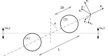
The situation investigated here is sketched in figure 1. Two spheres of equal radius
 $R$
, separated by a centre-to-centre distance
 $L$
are subjected to an oscillating flow of amplitude
 $u_{a}$
, angular frequency
 $\unicode[STIX]{x1D714}$
and angle
 $\unicode[STIX]{x1D703}$
with respect to the axis passing through the sphere centres. Both a Cartesian frame (
 $\boldsymbol{e}_{x},\boldsymbol{e}_{y},\boldsymbol{e}_{z}$
) and a cylindrical frame
 $(\boldsymbol{e}_{r},\boldsymbol{e}_{\unicode[STIX]{x1D711}},\boldsymbol{e}_{z})$
are used.
Sketch of the situation.

The whole flow is assumed to be incompressible, valid when the wavelength of the acoustic field is much larger than the size and spacing of the particles. The fluid has density
 $\unicode[STIX]{x1D70C}$
and kinematic viscosity
 $\unicode[STIX]{x1D708}$
.
The flow is governed by two non-dimensional parameters, the Reynolds number
 $Re=Ru_{a}/\unicode[STIX]{x1D708}$
and the Stokes number
 $\unicode[STIX]{x1D6FA}=\unicode[STIX]{x1D714}R^{2}/\unicode[STIX]{x1D708}$
. With the addition of the geometric parameters
 $L/R$
and
 $\unicode[STIX]{x1D703}$
, there are four parameters to consider.
The flow is represented by the state vector
 $\boldsymbol{q}=[\boldsymbol{u};p]$
which regroups the velocity field
 $\boldsymbol{u}$
and pressure field
 $p$
. This flow is governed by the incompressible Navier–Stokes equation which is conveniently written as
 $$\begin{eqnarray}{\mathcal{L}}\boldsymbol{q}=\frac{{\mathcal{C}}(\boldsymbol{q},\boldsymbol{q})}{2}.\end{eqnarray}$$
Here
 ${\mathcal{L}}$
is a linear operator and
 ${\mathcal{C}}$
is the nonlinear convection operator, defined as
 $$\begin{eqnarray}\displaystyle & \displaystyle {\mathcal{L}}[\boldsymbol{u};p]=\left[\begin{array}{@{}cc@{}}\unicode[STIX]{x1D708}\unicode[STIX]{x1D6E5}-\unicode[STIX]{x2202}_{t} & -\unicode[STIX]{x1D70C}^{-1}\unicode[STIX]{x1D735}\\ \unicode[STIX]{x1D735} & 0\end{array}\right][\boldsymbol{u};p], & \displaystyle\end{eqnarray}$$
 $$\begin{eqnarray}\displaystyle & \displaystyle {\mathcal{C}}([\boldsymbol{a};p_{a}],[\boldsymbol{b};p_{b}])=[\boldsymbol{a}\boldsymbol{\cdot }\unicode[STIX]{x1D735}\boldsymbol{b}+\boldsymbol{b}\boldsymbol{\cdot }\unicode[STIX]{x1D735}\boldsymbol{a};0]. & \displaystyle\end{eqnarray}$$
Far from the spheres (for
 $(r,z)\rightarrow \infty$
), the velocity field must match the applied uniform oscillating flow defined as
 $$\begin{eqnarray}\displaystyle & \displaystyle \boldsymbol{u}\approx u_{a}[\cos \unicode[STIX]{x1D703}\,\boldsymbol{e}_{z}+\sin \unicode[STIX]{x1D703}\,\boldsymbol{e}_{x}]\cos \unicode[STIX]{x1D714}t, & \displaystyle\end{eqnarray}$$
 $$\begin{eqnarray}\displaystyle & \displaystyle p\approx \unicode[STIX]{x1D70C}u_{a}\unicode[STIX]{x1D714}[z\cos \unicode[STIX]{x1D703}+x\sin \unicode[STIX]{x1D703}]\sin \unicode[STIX]{x1D714}t. & \displaystyle\end{eqnarray}$$
Assuming that the spheres are fixed (an hypothesis which will be discussed again in § 2.3), the velocity field also verifies a no-slip condition
 $\boldsymbol{u}=\mathbf{0}$
along their surface.
The forces exerted on each of the spheres (labelled
 $(1)$
and
 $(2)$
as in figure 1), are given by
 $$\begin{eqnarray}\boldsymbol{F}^{(1,2)}=\int _{{\mathcal{S}}_{1,2}}[-p\boldsymbol{n}+\unicode[STIX]{x1D70C}\unicode[STIX]{x1D708}(\unicode[STIX]{x1D735}\boldsymbol{u}+\unicode[STIX]{x1D735}\boldsymbol{u}^{T})\boldsymbol{\cdot }\boldsymbol{n}]\,\text{d}S,\end{eqnarray}$$
where
 ${\mathcal{S}}_{1,2}$
is the surface of the corresponding sphere.
2.2 Weakly nonlinear development
In the following, the problem is solved in non-dimensional form by setting
 $R=1$
,
 $\unicode[STIX]{x1D70C}=1$
,
 $\unicode[STIX]{x1D708}=1$
. The assumption that the amplitude of the oscillating field
 $u_{a}$
is small then implies
 $Re\ll 1$
, so it is convenient to conduct an asymptotic analysis in terms of this parameter. Retaining up to second-order terms, the flow is thus expanded as:
 $$\begin{eqnarray}\boldsymbol{q}=Re\,\boldsymbol{q}_{1}+Re^{2}\,\boldsymbol{q}_{2}+O(Re^{3}).\end{eqnarray}$$
The force exerted on each sphere can be similarly expanded, such that
 $$\begin{eqnarray}\boldsymbol{F}^{(1,2)}=Re\,\boldsymbol{F}_{1}^{(1,2)}+Re^{2}\,\boldsymbol{F}_{2}^{(1,2)},\end{eqnarray}$$
which means, in dimensional terms,
 $$\begin{eqnarray}\boldsymbol{F}^{(1,2)}\equiv \unicode[STIX]{x1D70C}\unicode[STIX]{x1D708}Ru_{a}\,\boldsymbol{F}_{1}^{(1,2)}+\unicode[STIX]{x1D70C}R^{2}u_{a}^{2}\,\boldsymbol{F}_{2}^{(1,2)}.\end{eqnarray}$$
Note that the order-one contribution to the force
 $\boldsymbol{F}_{1}^{(1,2)}$
is the direct response to the harmonic forcing, so it is periodic with frequency
 $\unicode[STIX]{x1D714}$
. The order-two contribution to the force
 $\boldsymbol{F}_{2}^{(1,2)}$
contains both a steady term and an unsteady term with frequency
 $2\unicode[STIX]{x1D714}$
. The latter will not be considered here as only the time average of the force is of interest.
Far away from the spheres (for
 $(r,z)\rightarrow \infty$
), the solution at order one must match with the applied uniform oscillating flow given by (2.4). Using cylindrical coordinates, this takes the following form for the velocity field:
 $$\begin{eqnarray}\boldsymbol{u}_{1}\approx \left(\frac{\cos \unicode[STIX]{x1D703}}{2}\boldsymbol{e}_{z}+\frac{\sin \unicode[STIX]{x1D703}}{4}[\text{e}^{\text{i}\unicode[STIX]{x1D711}}+\text{e}^{-\text{i}\unicode[STIX]{x1D711}}]\boldsymbol{e}_{r}+\frac{\text{i}\sin \unicode[STIX]{x1D703}}{4}[\text{e}^{\text{i}\unicode[STIX]{x1D711}}-\text{e}^{-\text{i}\unicode[STIX]{x1D711}}]\boldsymbol{e}_{\unicode[STIX]{x1D711}}\right)(\text{e}^{\text{i}\unicode[STIX]{x1D6FA}t}+\text{e}^{-\text{i}\unicode[STIX]{x1D6FA}t}).\end{eqnarray}$$
Therefore the solution at order one of the form
 $$\begin{eqnarray}\displaystyle \boldsymbol{q}_{1} & = & \displaystyle \cos \unicode[STIX]{x1D703}[\boldsymbol{q}_{A}\text{e}^{\text{i}\unicode[STIX]{x1D6FA}t}+(\boldsymbol{q}_{A})^{\ast }\text{e}^{-\text{i}\unicode[STIX]{x1D6FA}t}]+\sin \unicode[STIX]{x1D703}\nonumber\\ \displaystyle & & \displaystyle \times \,[\boldsymbol{q}_{T+}\text{e}^{+\text{i}\unicode[STIX]{x1D711}+\unicode[STIX]{x1D6FA}t}+\boldsymbol{q}_{T-}\text{e}^{-\text{i}\unicode[STIX]{x1D711}+\unicode[STIX]{x1D6FA}t}+(\boldsymbol{q}_{T+})^{\ast }\text{e}^{-\text{i}\unicode[STIX]{x1D711}-\text{i}\unicode[STIX]{x1D6FA}t}+(\boldsymbol{q}_{T-})^{\ast }\text{e}^{+\text{i}\unicode[STIX]{x1D711}-\text{i}\unicode[STIX]{x1D6FA}t}]\end{eqnarray}$$
is sought, where asterisks denote the complex conjugates of the corresponding terms. Here
 $\boldsymbol{q}_{A}$
is the first-order oscillating flow around two spheres in an axial configuration (
 $\unicode[STIX]{x1D703}=0$
) while
 $\boldsymbol{q}_{T+}$
and
 $\boldsymbol{q}_{T-}$
correspond to the first-order oscillating flow in a transverse configuration (
 $\unicode[STIX]{x1D703}=\unicode[STIX]{x03C0}/2$
). The general solution is a linear superposition of these components.
The first-order flow for axial oscillations
 $\boldsymbol{q}_{A}$
is the solution of the following linear system and associated boundary conditions:
 $$\begin{eqnarray}{\mathcal{L}}_{0}^{\unicode[STIX]{x1D6FA}}(\boldsymbol{q}_{A})=0;\quad \boldsymbol{q}_{A}\approx [0,0,1/2,\text{i}\unicode[STIX]{x1D6FA}x/2]\text{ as }(r,z)\rightarrow \infty ,\end{eqnarray}$$
Here
 ${\mathcal{L}}_{m}^{\unicode[STIX]{x1D6FA}}$
is the linear operator defined in (2.2), with temporal derivatives replaced by
 $\text{i}\unicode[STIX]{x1D6FA}$
,
 $\unicode[STIX]{x1D708}$
and
 $\unicode[STIX]{x1D70C}$
by 1, and azimuthal derivatives by
 $\text{i}m$
.
Using (2.6), the first-order flow
 $\boldsymbol{q}_{A}$
contributes to a force on the sphere labelled (1) and noted
 $\boldsymbol{F}_{1}^{(1)}=F_{A}\boldsymbol{e}_{z}\text{e}^{\text{i}\unicode[STIX]{x1D6FA}t}$
. The force exerted on the sphere labelled (2) can be deduced from symmetry considerations. Namely, the field
 $\boldsymbol{q}_{A}$
is antisymmetric with respect to the
 $z$
-axis, which means, for the pressure component, that
 $p_{A}(r,z)=-p_{A}(r,-z)$
. The same is true for the normal stress component entering the expression of the force. Considering that the axial projection of the normal vector is also antisymmetric, namely
 $n_{z}(r,z)=-n_{z}(r,-z)$
, this implies that the force felt by both spheres is the same.
Similarly, the two components describing the first-order field for transverse oscillations are the solutions of the following problems and associated boundary conditions:
 $$\begin{eqnarray}\displaystyle & \displaystyle {\mathcal{L}}_{1}^{\unicode[STIX]{x1D6FA}}(\boldsymbol{q}_{T+})=0;\quad \boldsymbol{q}_{T+}\approx [1/4,\text{i}/4,0,\text{i}\unicode[STIX]{x1D6FA}r/4]\text{ as }(r,z)\rightarrow \infty ; & \displaystyle\end{eqnarray}$$
 $$\begin{eqnarray}\displaystyle & \displaystyle {\mathcal{L}}_{-1}^{\unicode[STIX]{x1D6FA}}(\boldsymbol{q}_{T-})=0;\quad \boldsymbol{q}_{T-}\approx [1/4,-\text{i}/4,0,\text{i}\unicode[STIX]{x1D6FA}r/4]\text{ as }(r,z)\rightarrow \infty . & \displaystyle\end{eqnarray}$$
Using (2.6), the field
 $\boldsymbol{q}_{T+}\text{e}^{\text{i}\unicode[STIX]{x1D711}}+\boldsymbol{q}_{T-}\text{e}^{-\text{i}\unicode[STIX]{x1D711}}$
contributes to a force on the sphere labelled (1) noted
 $\boldsymbol{F}_{1}^{(1)}=F_{T}\boldsymbol{e}_{x}\text{e}^{\text{i}\unicode[STIX]{x1D6FA}t}$
. The force exerted on the sphere labelled (2) can again be deduced from symmetry considerations. Here, the fields
 $\boldsymbol{q}_{T\pm }$
are symmetric with respect to the
 $z$
-axis, which means, for the pressure components,
 $p_{T\pm }(r,z)=p_{T\pm }(r,-z)$
. The
 $x$
-component of the normal vector being also symmetric, this implies again that the force felt by both spheres is the same.
Gathering all contributions and taking into account the symmetry conditions, the order-one forces exerted on the spheres are thus given by:
 $$\begin{eqnarray}\boldsymbol{F}_{1}^{(1)}=\boldsymbol{F}_{1}^{(2)}=(F_{A}\cos \unicode[STIX]{x1D703}\,\boldsymbol{e}_{z}+F_{T}\sin \unicode[STIX]{x1D703}\,\boldsymbol{e}_{x})\text{e}^{\text{i}\unicode[STIX]{x1D6FA}t}+\text{c.c.}\end{eqnarray}$$
Note that
 $F_{A}$
and
 $F_{T}$
are complex numbers, implying a phase shift between the imposed oscillation and the exerted force. At this point we may also note that the fact that the oscillating force is equal on both spheres implies that, if they were allowed to move, they would oscillate in phase and with the same amplitude under the effect of this order-one force. We will discuss further the possible motion of the sphere in the next subsection.
The second-order term in (2.7) is obtained by substituting the solution at order one into the Navier–Stokes equations. Expressing the solution at order one in cylindrical coordinates allows the solution
 $\boldsymbol{q}_{2}\equiv [\boldsymbol{u}_{2},p_{2}]$
to be found as
 $$\begin{eqnarray}\displaystyle \boldsymbol{q}_{2} & = & \displaystyle \cos ^{2}\unicode[STIX]{x1D703}\,\boldsymbol{q}_{AA}^{0}\nonumber\\ \displaystyle & & \displaystyle +\,\sin ^{2}\unicode[STIX]{x1D703}[\boldsymbol{q}_{TT}^{0}+\boldsymbol{q}_{TT}^{2}\text{e}^{2\text{i}\unicode[STIX]{x1D711}}+(\boldsymbol{q}_{TT}^{2})^{\ast }\text{e}^{-2\text{i}\unicode[STIX]{x1D711}}]\nonumber\\ \displaystyle & & \displaystyle +\,\cos \unicode[STIX]{x1D703}\sin \unicode[STIX]{x1D703}[\boldsymbol{q}_{AT}^{1}\text{e}^{\text{i}\unicode[STIX]{x1D711}}+(\boldsymbol{q}_{AT}^{1})^{\ast }\text{e}^{-\text{i}\unicode[STIX]{x1D711}}]\nonumber\\ \displaystyle & & \displaystyle +\,\text{ (unsteady terms)}.\end{eqnarray}$$
The unsteady terms regroup into terms with temporal dependence
 $\text{e}^{\pm 2\text{i}\unicode[STIX]{x1D714}t}$
and azimuthal dependence
 $\text{e}^{0}$
,
 $\text{e}^{\pm \text{i}\unicode[STIX]{x1D711}}$
and
 $\text{e}^{\pm 2\text{i}\unicode[STIX]{x1D711}}$
. They are neglected as only the steady part of the second-order flow and associated steady forces are of interest.
The first term
 $\boldsymbol{q}_{AA}^{0}$
in (2.16) corresponds to the nonlinear interaction of the first-order axial flow
 $\boldsymbol{q}_{A}$
with itself. This flow is the solution of the following linear problem:
 $$\begin{eqnarray}{\mathcal{L}}_{0}^{0}(\boldsymbol{q}_{AA}^{0})={\mathcal{C}}_{0,0}(\boldsymbol{q}_{A},(\boldsymbol{q}_{A})^{\ast }),\end{eqnarray}$$
where
 ${\mathcal{C}}_{m_{a},m_{b}}(\boldsymbol{q}_{a},\boldsymbol{q}_{b})$
is as defined in (2.3) but with azimuthal derivatives of
 $\boldsymbol{q}_{a}$
replaced by
 $\text{i}m_{a}$
and azimuthal derivatives of
 $\boldsymbol{q}_{b}$
replaced by
 $\text{i}m_{b}$
.
This term
 $\boldsymbol{q}_{AA}^{0}$
contributes to a force on the sphere (1) directed in the axial
 $(z)$
direction and noted
 $F_{AA}$
. Note that the forcing term
 ${\mathcal{C}}_{1,-1}(\boldsymbol{q}_{A},(\boldsymbol{q}_{A})^{\ast })$
is symmetrical with respect to the
 $z$
-axis, so the field
 $\boldsymbol{q}_{AA}^{0}$
verifies the same property, i.e. for the pressure field
 $p_{AA}(r,z)=p_{AA}(r,-z)$
. Reminding that
 $n_{z}(r,z)=-n_{z}(r,-z)$
, this means that the force exerted on sphere (2) is opposite to that on sphere (1).
The terms in the second line of (2.16) correspond to the nonlinear interaction of the first-order transverse flow
 $\boldsymbol{q}_{T\pm }$
with itself. Note that the solution to this problem involves both an axisymmetric (with azimuthal wavenumber
 $0$
) and a non-axisymmetric contribution (with azimuthal wavenumber
 $\pm 2$
), respectively given by
 $$\begin{eqnarray}\displaystyle & {\mathcal{L}}_{0}^{0}(\boldsymbol{q}_{TT}^{00})={\mathcal{C}}_{1,-1}(\boldsymbol{q}_{T+},(\boldsymbol{q}_{T+})^{\ast })+{\mathcal{C}}_{-1,1}(\boldsymbol{q}_{T-},(\boldsymbol{q}_{T-})^{\ast }), & \displaystyle\end{eqnarray}$$
 $$\begin{eqnarray}\displaystyle & {\mathcal{L}}_{2}^{0}(\boldsymbol{q}_{TT}^{20})={\mathcal{C}}_{1,1}(\boldsymbol{q}_{T+},(\boldsymbol{q}_{T+})^{\ast }). & \displaystyle\end{eqnarray}$$
As the integrals of any term with azimuthal dependency
 $\text{e}^{\pm 2\text{i}\unicode[STIX]{x1D711}}$
along the surfaces of the spheres vanish, only the axisymmetric contribution to the field
 $\boldsymbol{q}_{TT}^{00}$
contributes to a force. The latter is exerted in the axial
 $(z)$
direction and noted
 $F_{TT}$
for sphere (1). The field
 $\boldsymbol{q}_{TT}^{00}$
verifying the same symmetry properties as
 $\boldsymbol{q}_{AA}^{0}$
, the force exerted on sphere (2) is again opposite to that on sphere (1).
The last term in (2.16) corresponds to an interaction between the axial and transverse parts of the solution at order one, and hence is present in any oblique configuration
 $\unicode[STIX]{x1D703}\neq (0,\unicode[STIX]{x03C0}/2)$
. It is given by the solution of
 $$\begin{eqnarray}{\mathcal{L}}_{1}^{0}(\boldsymbol{q}_{AT}^{1})={\mathcal{C}}_{0,1}(\boldsymbol{q}_{A},(\boldsymbol{q}_{T-})^{\ast })+{\mathcal{C}}_{0,1}((\boldsymbol{q}_{A})^{\ast },\boldsymbol{q}_{T+}).\end{eqnarray}$$
This last term contributes to a force in the transverse
 $(x)$
direction, noted
 $F_{AT}$
for the sphere labelled (1). Noting that
 $\boldsymbol{q}_{AT}^{1}$
is antisymmetric and that the
 $x$
-component of the normal is symmetric, this implies that the force on sphere (2) is opposite to that on sphere (1).
Gathering all these results, we are now in position to give an expression for the time-averaged force felt by the spheres
 $\overline{\boldsymbol{F}^{(1,2)}}$
. As given by (2.9), this corresponds to the steady part of
 $\boldsymbol{F}_{2}^{(1,2)}$
, which contain three contributions noted
 $F_{AA}$
,
 $F_{TT}$
and
 $F_{AT}$
. Taking into account the symmetry considerations discussed above, and reverting to dimensional form, we end up with the following expression:
 $$\begin{eqnarray}\overline{\boldsymbol{F}^{(1)}}=-\overline{\boldsymbol{F}^{(2)}}=\unicode[STIX]{x1D70C}R^{2}u_{a}^{2}[\cos ^{2}\unicode[STIX]{x1D703}\,F_{AA}\,\boldsymbol{e}_{z}+\sin ^{2}\unicode[STIX]{x1D703}\,F_{TT}\,\boldsymbol{e}_{z}+\cos \unicode[STIX]{x1D703}\sin \unicode[STIX]{x1D703}\,F_{AT}\,\boldsymbol{e}_{x}].\end{eqnarray}$$
2.3 Discussion: generalization to oscillating spheres
The whole derivation presented above was done under the assumption that the spheres are fixed and embedded in an external oscillating flow of amplitude
 $u_{a}$
. Before showing results, we discuss here the more general case where the spheres are oscillating in phase with each other with a velocity amplitude
 $u_{b}$
.
Let us consider first the most simple case where the spheres are driven in oscillation in a quiescent medium (
 $u_{b}\neq 0,u_{a}=0$
). Working in a relative frame moving with the particles, the equations of motions are the same as in the problem otherwise considered here, except for an additional uniform term
 $\unicode[STIX]{x2202}u_{b}/\unicode[STIX]{x2202}t$
corresponding to the relative acceleration of the non-inertial frame. This term modifies the pressure field of the order-one solution, and hence the unsteady force (2.15) is modified by the presence of an added-mass contribution. On the other hand, it has no effect on the steady order-two solution which remains exactly the same as written in the previous section.
In the more general case where the particles are moving under the effect of the acoustic forcing (
 $u_{a}\neq 0$
;
 $u_{b}\neq 0$
), the argument remains valid. In particular, the steady force exerted on the spheres is still given by (2.21), except that the overall scaling is the square of the relative velocity
 $|u_{b}-u_{a}|^{2}$
instead of
 $u_{a}^{2}$
.
In practice, if the spheres are freely moving,
 $u_{b}$
has to be deduced from the forcing
 $u_{a}$
by a dynamic equation relating the acceleration of the spheres to the forces exerted on them (given by (2.15) and including an added-mass contribution). Resolution of this problem clearly depends upon the mass of the spheres. Since the main focus of the present paper is on the steady streaming and steady forces, we leave a more detailed discussion of unsteady motion of spheres of arbitrary masses under the effect of acoustic forcing for a future study.
2.4 Numerical methods
All of the problems introduced are of the form
 ${\mathcal{L}}_{m}^{\unicode[STIX]{x1D714}}[\boldsymbol{u},p]=(\boldsymbol{V}\boldsymbol{F},0)$
where
 $\boldsymbol{V}\boldsymbol{F}$
is a volumetric forcing term. These problems are solved using finite elements. The equations are multiplied by test functions
 $[\boldsymbol{v},q]$
and integrated over the domain. Integration by parts is used for the Laplacian and pressure gradient terms which naturally leads to a no-traction condition
 $-p\boldsymbol{n}+\unicode[STIX]{x1D707}\unicode[STIX]{x1D735}\boldsymbol{u}\boldsymbol{\cdot }\boldsymbol{n}=\mathbf{0}$
on the boundaries of the computational domain.
To impose the velocity
 $\boldsymbol{u}=\boldsymbol{u}_{b}$
on some boundary
 $\unicode[STIX]{x1D6E4}$
of the domain, penalization terms are added of the form
 $1/\unicode[STIX]{x1D716}\int _{\unicode[STIX]{x1D6E4}}(\boldsymbol{u}-\boldsymbol{u}_{b})\boldsymbol{\cdot }\boldsymbol{v}\,r\,\text{d}s$
with
 $\unicode[STIX]{x1D716}\approx 10^{-10}$
to the variational formulation. Such penalization terms are required at the surfaces of the sphere to impose the no-slip condition for all problems, and at the outer boundary of the domain for the order-one problems to impose matching with the outer oscillating flow. For the order-two problems, no penalization terms are introduced, leading to a no-traction condition which is less restrictive than a no-slip condition.
A mesh was generated by triangulation over a circular domain (typically
 $40R$
) embedding the spheres. The mesh was refined in the vicinity of the spheres with typical grid size
 $0.03R$
. Mesh dependence was checked over various combinations of domain sizes and mesh densities, comprising of a refined inner circular region close to the sphere(s), and a coarser outer one further away. The results vary by
 ${<}1\%$
across all the meshes, when measuring forces
 $F_{TT}$
,
 $F_{AA}$
and
 $F_{AT}$
for all the range of
 $\unicode[STIX]{x1D6FA}$
tested.
The approach was validated in the case of a single sphere by comparing to the classical solution of Stokes (Reference Stokes1851) for the oscillating flow, and the asymptotic solutions of Riley (Reference Riley1966) for the steady streaming flow. In particular, as a consistency check, it was verified that the results for a single sphere are independent of the angle
 $\unicode[STIX]{x1D703}$
between the polar axis and the direction of oscillation.
3 Results
3.1 Flow structure
We first consider a high Stokes number case, corresponding to
 $\unicode[STIX]{x1D6FA}=100$
. In the case of particles with radius
 $R=100~\unicode[STIX]{x03BC}\text{m}$
in water, this corresponds to a frequency
 $f=\unicode[STIX]{x1D714}/2\unicode[STIX]{x03C0}\approx 1600~\text{Hz}$
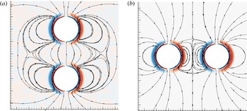
. Figure 2 shows the structure of the unsteady flow field
 $\boldsymbol{q}_{1}$
, for both axial and lateral configurations, in the case
 $L/R=4$
. The imaginary part of the flow field at the instant when the applied oscillation reverses sign is shown. The vorticity contours display the classical structure of a Stokes layer, with overlaid vorticity structures of opposite sign. At this instant of the cycle the flow forms closed streamlines with a toroidal shape around each of the spheres which are deformed by the presence of the other sphere, especially in the lateral configuration.
Oscillating flow around two spheres for
 $\unicode[STIX]{x1D6FA}=100$
:
 $(a)$
axial configuration, (b) lateral configuration. Streamlines and vorticity levels of the imaginary part.

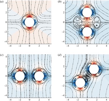
Streamlines and pressure contours of the steady streaming flow around one or two spheres for
 $\unicode[STIX]{x1D6FA}=100$
:
 $(a)$
single sphere, (b) two spheres in axial configuration, (c) two spheres in lateral configuration, (d) two spheres in oblique configuration. (
 $L/R=4$
in
 $(b{-}d)$
.)

Figure 3 shows the structure of the steady streaming flow
 $\boldsymbol{q}_{2}$
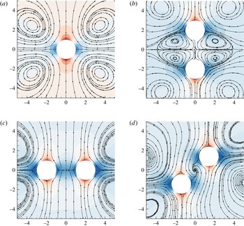
for the same parameters. The case of a single sphere is first depicted, and displays the characteristic structure identified by Lane (Reference Lane1955), with an outer flow being expelled away in the direction of the oscillation (vertical direction on the figure), and an inner flow characterized by vortical structures rotating in opposite directions. For two spheres, the inner flow around each of the spheres displays a pattern similar to that around a single one, but the two streaming flows interact to give rise to additional structures. Note that away from the spheres, in each of the cases displayed, the structure is more similar to that around a single sphere of larger dimension, with the flow being expelled away in the vertical direction. In the case of two spheres in axial configuration (figure 3
b), the flow is axisymmetric and the streamlines are closed. This is not true in the lateral configuration (figure 3
c) and the streamlines in the (
 $x{-}z$
) plane are clearly divergent in the region located between the spheres. This feature reveals a convergence of the flow in the perpendicular direction. Note also that in the four recirculation regions located between the spheres, the flow spirals inwards, indicating a divergence in the perpendicular direction. The oblique configuration (figure 5
d) is even more complex: here the convergence of the planar flow in the central region manifests through the existence of a focus with streamlines spiralling outwards, while in the two closer recirculation regions the flow spirals inwards.
This steady streaming flow exerts a non-zero mean force on the spheres. In the axial configuration (figure 3
b), this force is found to be repelling (
 $F_{AA}<0$
) while in the lateral configuration (figure 3
c), this force is attractive (
 $F_{TT}<0$
). This feature can be explained qualitatively by looking at the streamlines around a single sphere: since the outer flow is going outwards in the vertical direction, it seems logical that a second sphere located in this direction will feel a repelling force. Similarly, the flow generated by a single sphere goes inwards in the horizontal direction and thus a second sphere located in this direction will logically feel an attractive force.
Another indication of the direction of the force can be obtained by looking at the pressure isolevels associated with this sphere. Around a single sphere the pressure distribution is quadripolar and induces no net force. In the axial configuration, a close inspection shows that the regions of high pressure located between the spheres are more intense than the ones located outside, leading to a net repelling force. However in the lateral configuration, the regions of low pressure located between the spheres are reinforced, leading to a net attracting force. Finally, in the oblique configuration (figure 3 d), the force is transverse and tends to tilt the two spheres towards the transverse configuration.
Next, a low Stokes number case corresponding to
 $\unicode[STIX]{x1D6FA}=1$
,
 $L/R=4$
is investigated. In the case of particles with radius
 $R=100~\unicode[STIX]{x03BC}\text{m}$
in water, this corresponds to a frequency
 $f=\unicode[STIX]{x1D714}/2\unicode[STIX]{x03C0}\approx 1.6~\text{Hz}$
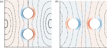
. In this range, viscous effects play a much larger role, and so the flow structure extends to a much larger region, as shown in figure 4. In particular, the vorticity is more diffuse and does not display the change of sign characteristic of a Stokes layer.
In the low-frequency range, the steady streaming flow around a single sphere (figure 5
a) has a different structure compared to the high-frequency range displayed previously, as it is characterized by a single set of vortical structures instead of two imbricated layers. Note that this trend is consistent with asymptotic predictions in the limit
 $\unicode[STIX]{x1D6FA}\ll 1$
from Riley (Reference Riley1966).
Oscillating flow around two spheres for
 $\unicode[STIX]{x1D6FA}=1$
: (a) axial configuration, (b) lateral configuration. Streamlines and vorticity levels of the imaginary part.

In the case of two spheres (figure 5 b–d), the interaction of the steady streaming induced by each sphere also leads to intricate flow patterns. Note that in this case, the force is attracting in the axial configuration and repelling in the transverse one. This can be explained either by a close inspection of the pressure isolevels, or by assuming qualitatively that each sphere feels the effect of the streaming flow generated by the other, which is vertically attractive and horizontally repulsive as soon as the spheres are close enough to fall within the inner region of the recirculating flow. Note that in the oblique configuration (figure 5 d), the force is transverse and tends to tilt the two spheres towards the transverse configuration, in the same way as in the high Stokes number regime.
Steady streaming flow around one or two spheres for
 $\unicode[STIX]{x1D6FA}=1$
: (a) single sphere, (b) two spheres in axial configuration, (c) two spheres in lateral configuration, (d) two spheres in oblique configuration. (
 $L/R=4$
in
 $(b{-}d)$
.)

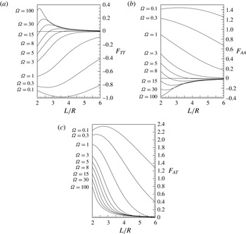
Forces exerted on the spheres due to steady streaming flow as function of the distance
 $L/R$
for various values of
 $\unicode[STIX]{x1D6FA}$
: (a) axial force in transverse oscillation
 $F_{TT}$
, (b) axial force in axial oscillation
 $F_{AA}$
, (c) transverse force in oblique oscillation
 $F_{AT}$
.

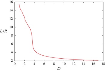
Distance between the sphere centres for the stable equilibrium in transverse configuration.

3.2 Steady forces at order two
As given by (2.6), the steady force felt by the spheres at order two is fully defined by the quantities
 $F_{AA},F_{TT}$
and
 $F_{AT}$
. Figure 6 shows the dependency of these forces when varying both the Stokes number
 $\unicode[STIX]{x1D6FA}$
and the distance
 $L/R$
between the spheres. The axial force in the transverse configuration
 $F_{TT}$
(figure 6
a) shows that for high frequencies, the force is always attractive while for low frequencies it is repulsive. For intermediate frequencies (
 $\unicode[STIX]{x1D6FA}=3$
to
 $15$
in the figure), the force is attractive at large distances but repulsive at small distances. Therefore, in this range of frequencies there exists a stable equilibrium position. The axial force in the axial configuration (figure 6
b) shows the opposite trends: for high frequencies, the force is always repulsive. For low frequencies it is attractive. For intermediate frequencies (
 $\unicode[STIX]{x1D6FA}=3$
to
 $15$
in the figure), the force is repulsive at large distances but attractive at small distances. Therefore, there is also an equilibrium position, but this one is unstable.
The contribution
 $F_{AT}$
to the force, which is present only in oblique configurations, is plotted on figure 6(c). This force being transverse and opposite on each of the spheres, it leads to a torque
 $LF_{AT}\sin \unicode[STIX]{x1D703}\cos \unicode[STIX]{x1D703}$
which would tend to cause their line-of-centres to rotate in the
 $(x,z)$
-plane if the spheres were allowed to move. Considering that
 $F_{AT}$
is always positive, this means that the torque will always tend to realign the spheres in the transverse direction.
Figure 7 shows the centre-to-centre distance between the spheres for the stable equilibrium situation in transverse configuration as a function of the Stokes number. For large enough frequencies (
 $\unicode[STIX]{x1D6FA}>20.1$
), there is no equilibrium position and the force remains attractive up to the point where the spheres touch each other (
 $L/R=2$
). In the limit of small frequencies, on the other hand, the equilibrium distance tends to infinity and the results can be fitted with the law
 $L/R\approx K/\unicode[STIX]{x1D6FA}$
where
 $K\simeq 16.5$
. Note that this asymptotic trend is similar to that observed in the experiment and numerical simulations of Klotsa et al. (Reference Klotsa, Swift, Bowley and King2007), but in this latter work the constant was
 $K\simeq 6.5$
(when expressed in the non-dimensionalization of this paper) during experiments, and
 $K\simeq 9$
in simulations. This difference may be attributed to the fact that in the experimental work the spheres were rolling upon a solid bottom, while here they are fully immersed in the fluid. In the numerical simulations of Klotsa et al. (Reference Klotsa, Swift, Bowley and King2007), the domain in the
 $z-$
direction was restricted to only
 $6R$
top to bottom, while here a domain of around
 $80R$
has been employed. It is likely that the difference in the result is due to the significant blockage effect in the simulations of Klotsa et al. (Reference Klotsa, Swift, Bowley and King2007).
4 Conclusion
In this work, the flow around two spheres subjected to a uniformly oscillating flow has been investigated using a perturbation method. The leading-order flow is oscillating, while the second-order flow contains a steady component referred to as the steady streaming flow. The structure of this flow has been described for axial, transverse and oblique configurations and is characterized by intricate patterns due to the interaction of the flows generated by each sphere. The mean forces exerted on the sphere have been characterized as a function of the Stokes number and the distance. In oblique configurations, the spheres are subjected to a torque which always tends to realign them perpendicularly to the direction of oscillation. In this transverse configuration, the force is always attractive in the high Stokes number regime and repulsive in the low Stokes number regime. For intermediate frequencies, there exists an equilibrium configuration where the force is zero. We emphasize that, although the analysis has been presented in the case where the spheres are assumed fixed in space, the general results of the study remain valid when taking into account their oscillatory motion due to the direct effect of the forcing.
For future studies, several extensions of the perturbation approach and the numerical method developed in this work present themselves. First, the whole approach is directly applicable to single non-spherical particles such as ellipsoids or cylinders, and to pairs of particles of unequal size. In the first case, one expects the microstreaming to exert a torque which tends to align the particle perpendicularly to the direction of oscillation. In the second case, one can expect the existence of an equilibrium state in which the two particles stay at a fixed distance from each other but migrate laterally. Secondly, in cases where the acoustic wavelength is comparable to the size of the particles and/or the amplitude of the acoustic field is large, the approach should be repeated in a compressible framework. This future analysis would allow description within a single approach of both the radiation forces responsible for primary migration of the particles within an acoustic field and the interaction forces due to microstreaming. Finally, the method can be applied to assess the motion and interaction of bubbles in an acoustic field.
Acknowledgements
This work was supported by the Australian Research Council Discovery Project DP150103177, the Swinburne Visiting Researcher Scheme, and the Institut National Polytechnique de Toulouse (INPT) under SMI grant.