1 Introduction
Some fluid processes in nature may be described using horizontal, two-dimensional (2D) mathematical models. Many geophysical flows, such as those in Earth’s atmosphere and oceans, occur on approximately horizontal layers whose vertical thickness is very small compared to the horizontal scale of motion (for example, Wayne Reference Wayne2011). In the balanced flow regime, void of inertia–gravity waves, and in the inviscid and adiabatic limit, the vertical, gravity oriented, velocity component is several orders of magnitude smaller than the horizontal velocity component. Under these circumstances the fluid tends to organize itself into coherent vortex structures such as mesoscale and submesoscale vortices, dipoles, tripoles, etc., which are, to a first approximation, horizontal structures (for example, McWilliams Reference McWilliams1984). Though most of these barotropic vortical flows develop also a baroclinic component, vertical density stratification and planetary rotation keep the flow to a large extent horizontal and balanced (for example, Dritschel & Viúdez Reference Dritschel and Viúdez2003). In such balanced flows, fluid particles move on slow-displacing, almost horizontal isopycnal surfaces. Fluid vertical velocity is, to the second order, quasigeostrophic approximation, mostly related to the horizontal density gradients, which themselves define the first-order, horizontal geostrophic velocity (Hoskins, Draghici & Davies Reference Hoskins, Draghici and Davies1978). Thus, the horizontal 2D flow is essential to correctly understand the more general three-dimensional structure. Hence the importance, particularly in geophysical fluid dynamics of balanced flows, of developing 2D mathematical models as a first step towards more complicated three-dimensional dynamics. The aim of this article is to provide exact vortex solutions of 2D inviscid Euler flows that may serve as a basis for more developed baroclinic models.
The approach followed here to obtain the vortex solutions may be described in three steps. In the first step (§ 2) we obtain interior, close to the vortex centre, stream flow solutions in polar coordinates
 $(r,\unicode[STIX]{x1D703})$
assuming separation of variables (
 $r$
,
 $\unicode[STIX]{x1D703}$
, and time
 $t$
) and azimuthal dependence, or azimuthal modes,
 $\text{exp}(\text{i}m\unicode[STIX]{x1D703})$
, where
 $m$
is the azimuthal wavenumber. Under these constraints the flow is steady and the radial solutions for the stream function
 $\unicode[STIX]{x1D713}(r,\unicode[STIX]{x1D703})$
are given by Bessel functions of the first kind
 $\text{J}_{m}(r)$
. Bessel functions
 $\text{J}_{m}(r)$
oscillate infinitely as
 $r$
increases, hence, the second step is limiting the interior solution to a radial boundary and finding the exterior potential flow solutions that confine the vortex vorticity to a finite region while keeping the velocity and vorticity fields continuous at the interior–exterior boundary radius. The extent of this radial boundary depends on the
 $n$
th zero of
 $\text{J}_{m}(r)$
, which defines the number of internal vorticity shells. The piecewise stream function consisting of interior and exterior flow solutions is thus completed. However, these steady piecewise solutions have a constant or infinite velocity as
 $r\rightarrow \infty$
. Hence, the third step (§ 3) consists of adding a background potential flow, applied to the complete domain, that sets to zero the velocity at infinity. The background flow turns the vorticity field unsteady. This third step is only completed for azimuthal wavenumbers
 $m=0$
and
 $m=1$
, because in these cases the background velocity field is a rigid motion that keeps the vorticity geometry unchanged, and the complete unsteady solution for the superposition of both modes (§ 4) is found. A particular Chaplygin–Lamb (C–L) dipole with continuous vorticity (Chaplygin Reference Chaplygin1903; Flierl, Stern & Whitehead Reference Flierl, Stern and Whitehead1983; Meleshko & van Heijst Reference Meleshko and van Heijst1994) is a particular case of this solution for
 $n=1$
.
2 Azimuthal solutions
As is usual in 2D isochoric flow, the field solutions are given in terms of a stream function
 $\unicode[STIX]{x1D713}(\boldsymbol{x},t)$
which provides the horizontal velocity
 $\boldsymbol{u}(\boldsymbol{x},t)$
and vorticity
 $\unicode[STIX]{x1D701}(\boldsymbol{x},t)$
,
 $$\begin{eqnarray}\boldsymbol{u}=-\unicode[STIX]{x1D735}\times (\unicode[STIX]{x1D713}\boldsymbol{k}),\quad \unicode[STIX]{x1D701}\equiv \boldsymbol{k}\boldsymbol{\cdot }\unicode[STIX]{x1D735}\times \boldsymbol{u}=\unicode[STIX]{x1D6FB}^{2}\unicode[STIX]{x1D713},\end{eqnarray}$$
where
 $\boldsymbol{k}$
is the vertical unit vector and
 $\unicode[STIX]{x1D735}$
is the 2D gradient operator. The fundamental dynamical equation is the material conservation of vorticity
 $$\begin{eqnarray}\frac{\text{d}\unicode[STIX]{x1D701}}{\text{d}t}=\frac{\unicode[STIX]{x2202}\unicode[STIX]{x1D701}}{\unicode[STIX]{x2202}t}+\boldsymbol{u}\boldsymbol{\cdot }\unicode[STIX]{x1D735}\unicode[STIX]{x1D701}=\frac{\unicode[STIX]{x2202}}{\unicode[STIX]{x2202}t}\unicode[STIX]{x1D6FB}^{2}\unicode[STIX]{x1D713}+{\mathcal{J}}\{\unicode[STIX]{x1D713},\unicode[STIX]{x1D6FB}^{2}\unicode[STIX]{x1D713}\}=0,\end{eqnarray}$$
where
 ${\mathcal{J}}\{A(x,y),B(x,y)\}=\unicode[STIX]{x2202}A/\unicode[STIX]{x2202}x\unicode[STIX]{x2202}B/\unicode[STIX]{x2202}y-\unicode[STIX]{x2202}B/\unicode[STIX]{x2202}x\unicode[STIX]{x2202}A/\unicode[STIX]{x2202}y$
is the Jacobian operator.
2.1 The interior flow
We seek solutions to (2.2) in terms of separation of polar coordinates
 $(r,\unicode[STIX]{x1D703})$
with a radial dependence function
 $R_{m}(r)$
, a time-dependent complex amplitude
 $\hat{T}(t)$
and azimuthal modes
 $\exp \{\text{i}m\unicode[STIX]{x1D703}\}$
,
 $$\begin{eqnarray}\unicode[STIX]{x1D713}_{m}(r,\unicode[STIX]{x1D703},t)=R_{m}(r)\text{e}^{\text{i}m\unicode[STIX]{x1D703}}\hat{T}_{m}(t).\end{eqnarray}$$
Azimuthal-mode solutions (2.3) satisfying material vorticity conservation (2.2) imply
 $\hat{T}_{m}^{\prime }(t)=0$
(appendix A). In this case the flow is steady and the amplitudes
 $\hat{T}_{m}(t)=\hat{\unicode[STIX]{x1D713}}_{m}$
are constant. Flow steadiness is not imposed, but it results as a dynamical consequence of assuming (2.3). Since the flow is steady, symbol
 $t$
is henceforth omitted from the list of independent variables and we write the mode-
 $m$
stream function
 $\unicode[STIX]{x1D713}_{m}$
as
 $$\begin{eqnarray}\unicode[STIX]{x1D713}_{m}(r,\unicode[STIX]{x1D703})=\hat{\unicode[STIX]{x1D713}}_{m}R_{m}(r)\text{e}^{\text{i}m\unicode[STIX]{x1D703}}.\end{eqnarray}$$
The local rate of change of vorticity
 $\unicode[STIX]{x2202}\unicode[STIX]{x1D701}/\unicode[STIX]{x2202}t=0$
, and therefore the material conservation of vorticity (2.2), reduces to the zero vorticity advection
 $\boldsymbol{u}\boldsymbol{\cdot }\unicode[STIX]{x1D735}\unicode[STIX]{x1D701}=0$
, in polar coordinates,
 $$\begin{eqnarray}\boldsymbol{u}\boldsymbol{\cdot }\unicode[STIX]{x1D735}\unicode[STIX]{x1D701}=u\frac{\unicode[STIX]{x2202}\unicode[STIX]{x1D701}}{\unicode[STIX]{x2202}r}+\frac{v}{r}\frac{\unicode[STIX]{x2202}\unicode[STIX]{x1D701}}{\unicode[STIX]{x2202}\unicode[STIX]{x1D703}}=0.\end{eqnarray}$$
Integration of (2.5) leads (appendix A) to the Bessel differential equation
 $$\begin{eqnarray}r^{2}R^{\prime \prime }(r)+rR^{\prime }(r)+R(r)(c_{0}^{2}r^{2}-m^{2})=0,\end{eqnarray}$$
where
 $c_{0}$
is an integration constant. The general solution to (2.6) involves Bessel functions of the first and second kinds, but only the Bessel function of the first kind
 $\text{J}_{m}(r)$
is finite at the origin point
 $r=0$
. The origin point must be included since it belongs to the domain of the interior solution. We define the dimensionless radial coordinate
 $\unicode[STIX]{x1D712}\equiv c_{0}r$
, and set the scale constant
 $c_{0}\equiv 1$
so that
 $\unicode[STIX]{x1D712}$
provides the vortex scale. The solutions to (2.6) are therefore the Bessel functions of the first kind
 $$\begin{eqnarray}R_{m}(r)=\text{J}_{m}(\unicode[STIX]{x1D712}),\end{eqnarray}$$
and the stream functions
 $\unicode[STIX]{x1D6F9}_{Im}$
of the interior flow (henceforth subscript
 $I$
) are explicitly, in polar coordinates,
 $$\begin{eqnarray}\unicode[STIX]{x1D6F9}_{Im}(\unicode[STIX]{x1D712},\unicode[STIX]{x1D703})=\hat{\unicode[STIX]{x1D713}}_{m}\text{J}_{m}(\unicode[STIX]{x1D712})\text{e}^{\text{i}m\unicode[STIX]{x1D703}}.\end{eqnarray}$$
The complex coefficient
 $\hat{\unicode[STIX]{x1D713}}_{m}$
defines both amplitude and spatial orientation of the vortical structures. We introduce also the
 $n$
th zero
 $j_{m,n}$
of the Bessel function
 $\text{J}_{m}(\unicode[STIX]{x1D712})$
 $$\begin{eqnarray}\text{J}_{m}(j_{m,n})=0,\quad m\geqslant 0,\,n\geqslant 1.\end{eqnarray}$$
To lighten the notation, subindices
 $m$
and
 $n$
may be omitted in those function symbols where its presence in results is obvious; however, they are included when necessary to unambiguously express the meaning of terms.
The velocity
 $\boldsymbol{u}_{Im}$
of the interior rotational flow, obtained from (2.1a
) and (2.8), is
 $$\begin{eqnarray}\boldsymbol{u}_{I}(\unicode[STIX]{x1D712},\unicode[STIX]{x1D703})=\hat{\unicode[STIX]{x1D713}}_{m}\text{e}^{\text{i}m\unicode[STIX]{x1D703}}\left(-\text{i}m\frac{\text{J}_{m}(\unicode[STIX]{x1D712})}{\unicode[STIX]{x1D712}}\boldsymbol{e}_{r}+\text{J}_{m}^{\prime }(\unicode[STIX]{x1D712})\boldsymbol{e}_{\unicode[STIX]{x1D703}}\right),\end{eqnarray}$$
where the derivative
 $\text{J}_{m}^{\prime }(\unicode[STIX]{x1D712})$
may be calculated from the recurrence relation
 $$\begin{eqnarray}2\text{J}_{m}^{\prime }(\unicode[STIX]{x1D712})=\text{J}_{m-1}(\unicode[STIX]{x1D712})-\text{J}_{m+1}(\unicode[STIX]{x1D712}).\end{eqnarray}$$
The radial component of
 $\boldsymbol{u}_{I}$
vanishes at the zeros
 $\unicode[STIX]{x1D712}=j_{m,n}$
(
 $u_{Im}(j_{m,n},\unicode[STIX]{x1D703})=0$
) but the azimuthal velocity does not (
 $v_{I}(j_{m,n},\unicode[STIX]{x1D703})\neq 0$
). Since the system of equations
 $\{\text{J}_{m}(\unicode[STIX]{x1D712}),\text{J}_{m}^{\prime }(\unicode[STIX]{x1D712})\}=\{0,0\}$
has no solutions for
 $\unicode[STIX]{x1D712}>0$
the stagnation lines are given by the nodes of
 $\text{Re}\{\hat{\unicode[STIX]{x1D713}}_{m}\exp (\text{i}m\unicode[STIX]{x1D703})\}$
. The interior vorticity, obtained from (2.1b
) and (2.8), is
 $$\begin{eqnarray}\unicode[STIX]{x1D701}_{Im}(\unicode[STIX]{x1D712},\unicode[STIX]{x1D703})=-\unicode[STIX]{x1D6F9}_{Im}(\unicode[STIX]{x1D712},\unicode[STIX]{x1D703}),\end{eqnarray}$$
which vanishes at
 $\unicode[STIX]{x1D712}=j_{m,n}$
. The Jacobian
 ${\mathcal{J}}\{a,b\}$
in (2.2) is a skew-symmetric bilinear form (
 ${\mathcal{J}}\{A,B\}+{\mathcal{J}}\{B,A\}=0$
) and, as a consequence of (2.12), the nonlinear advective terms cancel out,
 ${\mathcal{J}}\{\unicode[STIX]{x1D6F9}_{Ii},\unicode[STIX]{x1D6FB}^{2}\unicode[STIX]{x1D6F9}_{Ij}\}+{\mathcal{J}}\{\unicode[STIX]{x1D6F9}_{Ij},\unicode[STIX]{x1D6FB}^{2}\unicode[STIX]{x1D6F9}_{Ii}\}=-{\mathcal{J}}\{\unicode[STIX]{x1D6F9}_{Ii},\unicode[STIX]{x1D6F9}_{Ij}\}-{\mathcal{J}}\{\unicode[STIX]{x1D6F9}_{Ij},\unicode[STIX]{x1D6F9}_{Ii}\}=0$
, so that any combination of
 $N$
azimuthal modes
 $$\begin{eqnarray}\unicode[STIX]{x1D6F9}_{I}(\unicode[STIX]{x1D712},\unicode[STIX]{x1D703})=\mathop{\sum }_{m=0}^{N}\unicode[STIX]{x1D6F9}_{Im}(\unicode[STIX]{x1D712},\unicode[STIX]{x1D703})=\mathop{\sum }_{m=0}^{N}\hat{\unicode[STIX]{x1D713}}_{m}\text{J}_{m}(\unicode[STIX]{x1D712})\text{e}^{\text{i}m\unicode[STIX]{x1D703}},\end{eqnarray}$$
is a steady state solution of the material conservation of vorticity (2.2).
2.2 The exterior flow
To obtain vortices with bounded vorticity the spatial domain of the interior rotational flow
 $\boldsymbol{u}_{I}$
is limited to the circular region inside a given boundary radius
 $\unicode[STIX]{x1D712}_{l}$
. The flow solution must therefore be completed with an exterior potential flow satisfying the continuity conditions for velocity and vorticity at the vorticity boundary
 $\unicode[STIX]{x1D712}_{l}$
.
The exterior mode-0 flow is special since the interior flow is azimuthal and results as being convenient, for its latter application, to solve in a more general case, leaving aside the irrotational condition, and considering an arbitrary vorticity limit
 $\unicode[STIX]{x1D712}_{l}>0$
. The corresponding exterior stream function
 $\unicode[STIX]{x1D6F9}_{E0}(\unicode[STIX]{x1D712})$
(henceforth subscript
 $E$
) is obtained from the sum of an irrotational component (dependence
 $\ln \unicode[STIX]{x1D712}$
) and a constant vorticity component (dependence
 $\unicode[STIX]{x1D712}^{2}$
), yielding
 $\unicode[STIX]{x1D6F9}_{E0}(\unicode[STIX]{x1D712})=c_{0}+c_{1}\ln \unicode[STIX]{x1D712}+c_{2}\unicode[STIX]{x1D712}^{2}$
, where the constants
 $c_{i}$
are determined from the continuity boundary conditions for stream function
 $\unicode[STIX]{x1D6F9}_{E0}=\unicode[STIX]{x1D6F9}_{I0}$
, azimuthal velocity
 $\unicode[STIX]{x1D6F9}_{E0}^{\prime }=\unicode[STIX]{x1D6F9}_{I0}^{\prime }$
, and vorticity
 $\unicode[STIX]{x1D6F9}_{E0}^{\prime \prime }+\unicode[STIX]{x1D6F9}_{E0}^{\prime }/\unicode[STIX]{x1D712}=\unicode[STIX]{x1D6F9}_{I0}^{\prime \prime }+\unicode[STIX]{x1D6F9}_{I0}^{\prime }/\unicode[STIX]{x1D712}$
, at the vorticity limit
 $\unicode[STIX]{x1D712}=\unicode[STIX]{x1D712}_{l}$
. After rearranging terms the exterior stream function
 $\unicode[STIX]{x1D6F9}_{E0}$
is
 $$\begin{eqnarray}\frac{\unicode[STIX]{x1D6F9}_{E0}(\unicode[STIX]{x1D712})}{\unicode[STIX]{x1D713}_{0}}=\text{J}_{0}(\unicode[STIX]{x1D712}_{l})\left[1+\frac{\unicode[STIX]{x1D712}_{l}^{2}}{2}\ln \left(\frac{\unicode[STIX]{x1D712}}{\unicode[STIX]{x1D712}_{l}}\right)-\frac{\unicode[STIX]{x1D712}^{2}-\unicode[STIX]{x1D712}_{l}^{2}}{4}\right]-\text{J}_{1}(\unicode[STIX]{x1D712}_{l})\unicode[STIX]{x1D712}_{l}\ln \left(\frac{\unicode[STIX]{x1D712}}{\unicode[STIX]{x1D712}_{l}}\right),\quad \unicode[STIX]{x1D712}_{l}\leqslant \unicode[STIX]{x1D712},\end{eqnarray}$$
where the amplitude
 $\unicode[STIX]{x1D713}_{0}=\hat{\unicode[STIX]{x1D713}}_{0}\in \mathbb{R}$
.
The exterior mode-0 velocity,
 $\boldsymbol{u}_{Em,n}$
, obtained from (2.1a
) and (2.14), is
 $$\begin{eqnarray}\frac{\boldsymbol{u}_{E0}(\unicode[STIX]{x1D712})}{\unicode[STIX]{x1D713}_{0}}=\left[\frac{\text{J}_{0}(\unicode[STIX]{x1D712}_{l})}{2}\left(\frac{\unicode[STIX]{x1D712}_{l}^{2}}{\unicode[STIX]{x1D712}}-\unicode[STIX]{x1D712}\right)-\text{J}_{1}(\unicode[STIX]{x1D712}_{l})\frac{\unicode[STIX]{x1D712}_{l}}{\unicode[STIX]{x1D712}}\right]\boldsymbol{e}_{\unicode[STIX]{x1D703}},\quad \unicode[STIX]{x1D712}_{l}\leqslant \unicode[STIX]{x1D712}.\end{eqnarray}$$
The vorticity of the exterior mode-0 flow, obtained from (2.15), is constant
 $$\begin{eqnarray}\unicode[STIX]{x1D701}_{E0}=-\unicode[STIX]{x1D713}_{0}\text{J}_{0}(\unicode[STIX]{x1D712}_{l}),\quad \unicode[STIX]{x1D712}_{l}\leqslant \unicode[STIX]{x1D712},\end{eqnarray}$$
which matches the boundary condition
 $\unicode[STIX]{x1D701}_{E0}=\unicode[STIX]{x1D701}_{I0}(\unicode[STIX]{x1D712}_{l})$
, and vanishes at
 $\unicode[STIX]{x1D712}_{l}=j_{0,n}$
.
For modes
 $m\geqslant 1$
, the exterior stream functions
 $\unicode[STIX]{x1D6F9}_{Em,n}$
, are required to satisfy the boundary conditions at the radius
 $\unicode[STIX]{x1D712}_{l}=j_{m,n}$
(that is, where the velocity of the interior flow (2.10) is azimuthal). The stream function solutions (for example, Velasco Fuentes Reference Velasco Fuentes2000) are
 $$\begin{eqnarray}\frac{\unicode[STIX]{x1D6F9}_{E}(\unicode[STIX]{x1D712},\unicode[STIX]{x1D703})}{\hat{\unicode[STIX]{x1D713}}_{m}\text{e}^{\text{i}m\unicode[STIX]{x1D703}}}=\frac{\text{J}_{m-1}(j_{m,n})}{2m}j_{m,n}\left[\left(\frac{\unicode[STIX]{x1D712}}{j_{m,n}}\right)^{m}-\left(\frac{\unicode[STIX]{x1D712}}{j_{m,n}}\right)^{-m}\right],\quad j_{m,n}\leqslant \unicode[STIX]{x1D712}.\end{eqnarray}$$
The exterior potential flow
 $\boldsymbol{u}_{Em,n}$
, obtained from (2.1a
) and (2.17), is
 $$\begin{eqnarray}\displaystyle & & \displaystyle \frac{\boldsymbol{u}_{E}(\unicode[STIX]{x1D712},\unicode[STIX]{x1D703})}{\hat{\unicode[STIX]{x1D713}}_{m}\text{e}^{\text{i}m\unicode[STIX]{x1D703}}}=\frac{\text{J}_{m-1}(j_{m,n})}{2}\frac{j_{m,n}}{\unicode[STIX]{x1D712}}\nonumber\\ \displaystyle & & \displaystyle \quad \times \left\{-\text{i}\left[\left(\frac{\unicode[STIX]{x1D712}}{j_{m,n}}\right)^{m}-\left(\frac{\unicode[STIX]{x1D712}}{j_{m,n}}\right)^{-m}\right]\boldsymbol{e}_{r}+\left[\left(\frac{\unicode[STIX]{x1D712}}{j_{m,n}}\right)^{m}+\left(\frac{\unicode[STIX]{x1D712}}{j_{m,n}}\right)^{-m}\right]\boldsymbol{e}_{\unicode[STIX]{x1D703}}\right\},\quad j_{m,n}\leqslant \unicode[STIX]{x1D712}.\nonumber\\ \displaystyle & & \displaystyle\end{eqnarray}$$
For the rotational mode-0, the exterior velocity (2.18) gives also the correct velocity (2.15) only in the case
 $\unicode[STIX]{x1D712}_{l}=j_{0,n}$
. Using the recurrence identity of Bessel functions
 $$\begin{eqnarray}\text{J}_{m-1}(\unicode[STIX]{x1D712})+\text{J}_{m+1}(\unicode[STIX]{x1D712})=2m\frac{\text{J}_{m}(\unicode[STIX]{x1D712})}{\unicode[STIX]{x1D712}},\end{eqnarray}$$
it is deduced that the exterior flow (2.18) satisfies the boundary conditions at
 $\unicode[STIX]{x1D712}=j_{m,n}$
,
 $$\begin{eqnarray}\boldsymbol{u}_{E}(j_{m,n},\unicode[STIX]{x1D703})=\boldsymbol{u}_{I}(j_{m,n},\unicode[STIX]{x1D703})=\hat{\unicode[STIX]{x1D713}}_{m}\text{J}_{m-1}(j_{m,n})\text{e}^{\text{i}m\unicode[STIX]{x1D703}}\boldsymbol{e}_{\unicode[STIX]{x1D703}}.\end{eqnarray}$$
The exterior flow
 $\boldsymbol{u}_{Em,n}$
(
 $m\geqslant 1$
) is irrotational,
 $$\begin{eqnarray}\unicode[STIX]{x1D701}_{Em,n}(\unicode[STIX]{x1D712},\unicode[STIX]{x1D703})=\unicode[STIX]{x1D6FB}^{2}\unicode[STIX]{x1D6F9}_{Em,n}=0,\quad j_{m,n}\leqslant \unicode[STIX]{x1D712},\end{eqnarray}$$
a property that, due to (2.12), automatically satisfies vorticity continuity at
 $\unicode[STIX]{x1D712}=j_{m,n}$
(that is,
 $\unicode[STIX]{x1D701}_{Im}(j_{m,n},\unicode[STIX]{x1D703})=\unicode[STIX]{x1D701}_{Em,n}(j_{m,n},\unicode[STIX]{x1D703})=0$
).
2.3 The piecewise flow
Once the interior and exterior solutions have been obtained, the complete stream function
 $\widehat{\unicode[STIX]{x1D6F9}}$
is the piecewise function
 $$\begin{eqnarray}\widehat{\unicode[STIX]{x1D6F9}}_{m,n}(\unicode[STIX]{x1D712},\unicode[STIX]{x1D703})=\left\{\begin{array}{@{}ll@{}}\unicode[STIX]{x1D6F9}_{Im}(\unicode[STIX]{x1D712},\unicode[STIX]{x1D703}), & \unicode[STIX]{x1D712}\leqslant j_{m,n}\\ \unicode[STIX]{x1D6F9}_{Em,n}(\unicode[STIX]{x1D712},\unicode[STIX]{x1D703}), & j_{m,n}\leqslant \unicode[STIX]{x1D712},\end{array}\right.\end{eqnarray}$$
where the interior
 $\unicode[STIX]{x1D6F9}_{Im}$
and exterior
 $\unicode[STIX]{x1D6F9}_{Em}$
stream functions are given by (2.8) and (2.17) (or (2.14) for mode-0), respectively. Stream functions
 $\widehat{\unicode[STIX]{x1D6F9}}_{m,n}(\unicode[STIX]{x1D712},\unicode[STIX]{x1D703})$
are solutions to the fully nonlinear vorticity equation (2.2) and not only solutions to its linearized approximation. The piecewise vorticity
 $\widehat{\unicode[STIX]{x1D701}}_{m,n}$
, for
 $m=0$
and
 $m\geqslant 1$
, is simply
 $$\begin{eqnarray}\frac{\widehat{\unicode[STIX]{x1D701}}_{0,n}(\unicode[STIX]{x1D712})}{\unicode[STIX]{x1D713}_{0}}=\left\{\begin{array}{@{}ll@{}}-\text{J}_{0}(\unicode[STIX]{x1D712}), & \unicode[STIX]{x1D712}\leqslant \unicode[STIX]{x1D712}_{l}\\ -\text{J}_{0}(\unicode[STIX]{x1D712}_{l}), & \unicode[STIX]{x1D712}_{l}\leqslant \unicode[STIX]{x1D712},\end{array}\right.\quad \frac{\widehat{\unicode[STIX]{x1D701}}_{m,n}(\unicode[STIX]{x1D712},\unicode[STIX]{x1D703})}{\hat{\unicode[STIX]{x1D713}}_{m}\text{e}^{\text{i}m\unicode[STIX]{x1D703}}}=\left\{\begin{array}{@{}ll@{}}-\text{J}_{m}(\unicode[STIX]{x1D712}), & \unicode[STIX]{x1D712}\leqslant j_{m,n}\\ 0, & j_{m,n}\leqslant \unicode[STIX]{x1D712}.\end{array}\right.\end{eqnarray}$$
An example for
 $m=2$
and
 $n=1$
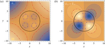
is shown in figure 1(a). The four vortices of the interior solution
 $\unicode[STIX]{x1D6F9}_{I2,1}$
are kept steady, in the vortex interior
 $\unicode[STIX]{x1D712}\leqslant j_{2,1}$
, surrounded by the exterior flow
 $\unicode[STIX]{x1D6F9}_{E2,1}$
. The stability and time evolution of this quadrupolar vortex was investigated by Velasco Fuentes (Reference Velasco Fuentes2000).
(a) The steady piecewise stream function
 $\widehat{\unicode[STIX]{x1D6F9}}_{2,1}$
. The black solid circle, with radius
 $\unicode[STIX]{x1D712}=j_{2,1}$
, separates the interior
 $\unicode[STIX]{x1D6F9}_{I2}$
from the exterior
 $\unicode[STIX]{x1D6F9}_{E2,1}$
solution. The vorticity contours coincide with those of
 $\widehat{\unicode[STIX]{x1D6F9}}_{2,1}$
in the interior region solution. Arrows indicate velocity direction. (b) The stream function
 $\widehat{\unicode[STIX]{x1D6F9}}_{2,1}+\bar{\unicode[STIX]{x1D6F9}}_{2,1}$
. The complex amplitude
 $\hat{\unicode[STIX]{x1D713}}_{2}=\text{i}$
. Blue colours in figures correspond to negative values.

3 Solutions with vanishing velocity at infinity
The steady piecewise flow solutions
 $\widehat{\boldsymbol{u}}_{m,n}\equiv -\unicode[STIX]{x1D735}\times (\widehat{\unicode[STIX]{x1D6F9}}_{m,n}\boldsymbol{k})$
have, as
 $\unicode[STIX]{x1D712}\rightarrow \infty$
, constant angular velocity (mode-0), constant velocity (mode-1), or tend to infinity (modes
 $m\geqslant 2$
). To provide flow solutions vanishing at infinity it is possible to add a background flow
 $\bar{\boldsymbol{u}}_{m,n}$
, applied to the complete spatial domain, such that the exterior velocity
 $\boldsymbol{u}_{Em,n}(\unicode[STIX]{x1D712},\unicode[STIX]{x1D703})\rightarrow \mathbf{0}$
as
 $\unicode[STIX]{x1D712}\rightarrow \infty$
. Advection of vorticity by
 $\bar{\boldsymbol{u}}_{m,n}$
will now cause unsteady vorticity fields. However, for modes
 $m=0$
and
 $m=1$
, this background flow is a rigid motion, which preserves the shape of the vorticity field, and becomes equivalent to a rotation (mode-0) or a translation (mode-1) of the reference frame.
3.1 The background flow
The stream function
 $\bar{\unicode[STIX]{x1D6F9}}$
of the background flow is obtained from the exterior stream function (2.17) at the limit
 $\unicode[STIX]{x1D712}\rightarrow \infty$
, while the background velocity
 $\bar{\boldsymbol{u}}$
may be obtained from the exterior velocity (2.18) at the limit
 $\unicode[STIX]{x1D712}\rightarrow \infty$
, or directly from
 $\bar{\unicode[STIX]{x1D6F9}}$
,
 $$\begin{eqnarray}\frac{\bar{\unicode[STIX]{x1D6F9}}_{m,n}(\unicode[STIX]{x1D712},\unicode[STIX]{x1D703})}{\hat{\unicode[STIX]{x1D713}}_{m}\text{e}^{\text{i}m\unicode[STIX]{x1D703}}}=-\frac{\text{J}_{m-1}(j_{m,n})}{2mj_{m,n}^{m-1}}\unicode[STIX]{x1D712}^{m},\quad \frac{\bar{\boldsymbol{u}}_{m,n}(\unicode[STIX]{x1D712},\unicode[STIX]{x1D703})}{\hat{\unicode[STIX]{x1D713}}_{m}\text{e}^{\text{i}m\unicode[STIX]{x1D703}}}=\frac{\text{J}_{m-1}(j_{m,n})}{2j_{m,n}^{m-1}}\unicode[STIX]{x1D712}^{m-1}(\text{i}\boldsymbol{e}_{r}-\boldsymbol{e}_{\unicode[STIX]{x1D703}}).\end{eqnarray}$$
The addition of
 $\widehat{\boldsymbol{u}}$
and
 $\bar{\boldsymbol{u}}$
is not a steady solution of the vorticity conservation (2.2) since these flows are steady and the advection of vorticity by the background flow
 $\bar{\boldsymbol{u}}\boldsymbol{\cdot }\unicode[STIX]{x1D735}\unicode[STIX]{x1D701}_{I}\neq 0$
.
Let us introduce the trajectory
 $\bar{\boldsymbol{r}}_{m,n}(\boldsymbol{X},t)$
of points
 $\boldsymbol{X}$
under the steady background flow
 $\bar{\boldsymbol{u}}_{m,n}(\boldsymbol{x})$
. Function
 $\bar{\boldsymbol{R}}\equiv \bar{\boldsymbol{r}}^{\unicode[STIX]{x1D704}}$
(subscripts
 $m,n$
omitted) is the inverse function of
 $\bar{\boldsymbol{r}}$
with respect to
 $\boldsymbol{x}$
(that is,
 $(\bar{\boldsymbol{r}}\circ \bar{\boldsymbol{R}})(\boldsymbol{x},t)=\boldsymbol{x}$
). The value
 $\bar{\boldsymbol{R}}(\boldsymbol{x},t)$
is the location at the reference time (here taken at
 $t=0$
) of the fluid particle located at
 $\boldsymbol{x}$
at time
 $t$
in the background flow. If the background velocity
 $\bar{\boldsymbol{u}}(\boldsymbol{x})$
is a rigid motion (only modes 0 and 1), the transformation
 $\boldsymbol{x}=\bar{\boldsymbol{r}}(\boldsymbol{X},t)$
represents a change of frame and in this case the transformed stream function
 $\widetilde{\unicode[STIX]{x1D6F9}}_{m,n}$
of the unsteady flow is
 $$\begin{eqnarray}\widetilde{\unicode[STIX]{x1D6F9}}_{m,n}(\boldsymbol{x},t)\equiv \widehat{\unicode[STIX]{x1D6F9}}_{m,n}(\bar{\boldsymbol{R}}(\boldsymbol{x},t))+\bar{\unicode[STIX]{x1D6F9}}_{m,n}(\boldsymbol{x}).\end{eqnarray}$$
The background stream function
 $\bar{\unicode[STIX]{x1D6F9}}_{m,n}(\boldsymbol{x})$
does not need to be transformed since, due to (2.1a
), it remains invariant to the change of frame associated with its own velocity. For modes
 $m\geqslant 2$
, stream functions
 $\widetilde{\unicode[STIX]{x1D6F9}}_{m,n}(\boldsymbol{x},t)$
are no longer time-independent solutions, though their distributions at
 $t=0$
, equivalent to
 $\widehat{\unicode[STIX]{x1D6F9}}_{m,n}(\boldsymbol{x})+\bar{\unicode[STIX]{x1D6F9}}_{m,n}(\boldsymbol{x})$
, may be useful to find time-dependent solutions. The example
 $\widetilde{\unicode[STIX]{x1D6F9}}_{2,1}(\boldsymbol{x},0)$
is shown in figure 1(b), which may be regarded as a head-on collision of two dipoles at the maximum closeness time.
For
 $m\leqslant 1$
, composing the steady
 $\widehat{\unicode[STIX]{x1D701}}(\boldsymbol{X})$
with
 $\bar{\boldsymbol{R}}$
yields the unsteady vorticity
 $$\begin{eqnarray}\widetilde{\unicode[STIX]{x1D701}}(\boldsymbol{x},t)\equiv (\widehat{\unicode[STIX]{x1D701}}\circ \bar{\boldsymbol{R}})(\boldsymbol{x},t)=\widehat{\unicode[STIX]{x1D701}}(\bar{\boldsymbol{R}}(\boldsymbol{x},t)),\end{eqnarray}$$
which represents the material conservation of vorticity for an observer moving with the background rigid flow
 $\bar{\boldsymbol{u}}$
or, equivalently, in the moving reference frame. For example, if the transformation is given in Cartesian coordinates
 $\bar{\boldsymbol{R}}_{m}(\boldsymbol{x},t)=\bar{X}_{m}(\boldsymbol{x},t)\boldsymbol{i}+\bar{Y}_{m}(\boldsymbol{x},t)\boldsymbol{j}$
, we may use polar coordinates, namely the initial radius
 $\bar{\unicode[STIX]{x1D6EF}}_{m}$
and phase
 $\bar{\unicode[STIX]{x1D6E9}}_{m}$
,
 $$\begin{eqnarray}\bar{\unicode[STIX]{x1D6EF}}_{m}(\boldsymbol{x},t)\equiv \sqrt{\bar{X}_{m}^{2}(\boldsymbol{x},t)+\bar{Y}_{m}^{2}(\boldsymbol{x},t)},\quad \bar{\unicode[STIX]{x1D6E9}}_{m}(\boldsymbol{x},t)\equiv \arctan \frac{\bar{Y}_{m}(\boldsymbol{x},t)}{\bar{X}_{m}(\boldsymbol{x},t)},\end{eqnarray}$$
to get the unsteady vorticity
 $\widetilde{\unicode[STIX]{x1D701}}$
in Cartesian coordinates from (2.23) using (3.3) and (3.4),
 $$\begin{eqnarray}\widetilde{\unicode[STIX]{x1D701}}_{m,n}(\boldsymbol{x},t)=\widehat{\unicode[STIX]{x1D701}}_{m,n}(\bar{\unicode[STIX]{x1D6EF}}_{m}(\boldsymbol{x},t),\bar{\unicode[STIX]{x1D6E9}}_{m}(\boldsymbol{x},t)).\end{eqnarray}$$
Expression (3.5) states that the vorticity of the fluid particle located at
 $(\boldsymbol{x},t)$
in the time-dependent flow equals the vorticity of the fluid particle located at
 $\boldsymbol{X}=\bar{\boldsymbol{R}}(\boldsymbol{x},t)$
in the steady flow, which here coincides with the unsteady flow at the reference time
 $t=0$
, or the reference flow configuration.
4 The mode-0+1 vortex: a particular C–L dipole
Although all azimuthal modes are solutions to (2.2), only modes 0 and 1 have far-field flows that are rigid motions. Since the superposition of interior solutions (2.13) is also a solution to the Euler equations, and the superposition of two rigid motions is also a rigid motion, the superposition of modes 0 and 1, with background flow given by a solid-body rotation and an uniform translation, is an unsteady nonlinear solution.
The background stream function
 $\bar{\unicode[STIX]{x1D6F9}}_{0}$
of the mode-0 is a rigid rotation with background angular velocity
 $\bar{\unicode[STIX]{x1D714}}_{0}$
given by
 $$\begin{eqnarray}\bar{\unicode[STIX]{x1D6F9}}_{0}(\unicode[STIX]{x1D712})\equiv \frac{\bar{\unicode[STIX]{x1D714}}_{0}}{2}\unicode[STIX]{x1D712}^{2},\quad \bar{\unicode[STIX]{x1D714}}_{0}\equiv \unicode[STIX]{x1D713}_{0}\frac{\text{J}_{0}(\unicode[STIX]{x1D712}_{l})}{2}.\end{eqnarray}$$
Choosing the vorticity limit
 $\unicode[STIX]{x1D712}_{l}=j_{0,n}$
implies
 $\bar{\unicode[STIX]{x1D6F9}}_{0}=0$
. The motion of points by the background flow is a rotation with
 $\bar{\unicode[STIX]{x1D6EF}}_{0}(\unicode[STIX]{x1D712})=\unicode[STIX]{x1D712}$
and
 $\bar{\unicode[STIX]{x1D6E9}}_{0}(\unicode[STIX]{x1D703},t)=\unicode[STIX]{x1D703}-\bar{\unicode[STIX]{x1D714}}_{0}t$
, and therefore the transformed stream function is
 $\widetilde{\unicode[STIX]{x1D6F9}}_{0}(\unicode[STIX]{x1D712})=\widehat{\unicode[STIX]{x1D6F9}}_{0}(\bar{\unicode[STIX]{x1D6EF}}_{0}(\unicode[STIX]{x1D712}))+\bar{\unicode[STIX]{x1D6F9}}_{0}(\unicode[STIX]{x1D712})$
, or explicitly, from (2.8), (2.14), and (4.1),
 $$\begin{eqnarray}\widetilde{\unicode[STIX]{x1D6F9}}_{0}(\unicode[STIX]{x1D712})=\unicode[STIX]{x1D713}_{0}\left\{\begin{array}{@{}ll@{}}\displaystyle \text{J}_{0}(\unicode[STIX]{x1D712})+\frac{\text{J}_{0}(\unicode[STIX]{x1D712}_{l})}{4}\unicode[STIX]{x1D712}^{2}, & \unicode[STIX]{x1D712}\leqslant \unicode[STIX]{x1D712}_{l}\\ \displaystyle \text{J}_{0}(\unicode[STIX]{x1D712}_{l})\left[1+\frac{\unicode[STIX]{x1D712}_{l}^{2}}{2}\ln \left(\frac{\unicode[STIX]{x1D712}}{\unicode[STIX]{x1D712}_{l}}\right)+\frac{\unicode[STIX]{x1D712}_{l}^{2}}{4}\right]-\text{J}_{1}(\unicode[STIX]{x1D712}_{l})\unicode[STIX]{x1D712}_{l}\ln \left(\frac{\unicode[STIX]{x1D712}}{\unicode[STIX]{x1D712}_{l}}\right), & \unicode[STIX]{x1D712}_{l}\leqslant \unicode[STIX]{x1D712},\end{array}\right.\end{eqnarray}$$
while, from (4.2), the non-vanishing vorticity is
 $$\begin{eqnarray}\widetilde{\unicode[STIX]{x1D701}}_{0}(\unicode[STIX]{x1D712})=\unicode[STIX]{x1D713}_{0}[\text{J}_{0}(\unicode[STIX]{x1D712}_{l})-\text{J}_{0}(\unicode[STIX]{x1D712})],\quad \unicode[STIX]{x1D712}\leqslant \unicode[STIX]{x1D712}_{l}.\end{eqnarray}$$
Modes 0 and 1 may be coupled, selecting now the vorticity limit of the mode-0 at
 $\unicode[STIX]{x1D712}_{l}=j_{1,n}$
, so that the background angular velocity (4.1b
) is
 $\bar{\unicode[STIX]{x1D714}}_{0}=\unicode[STIX]{x1D713}_{0}\text{J}_{0}(j_{1,n})/2$
. The background stream function of the mode-0+1 vortex
 $\bar{\unicode[STIX]{x1D6F9}}_{01}$
is the sum of the background stream functions of their respective modes
 $$\begin{eqnarray}\bar{\unicode[STIX]{x1D6F9}}_{01}(\boldsymbol{x})\equiv \bar{\unicode[STIX]{x1D6F9}}_{0}(\boldsymbol{x})+\bar{\unicode[STIX]{x1D6F9}}_{1}(\boldsymbol{x}),\end{eqnarray}$$
where
 $\bar{\unicode[STIX]{x1D6F9}}_{1}(\boldsymbol{x})$
is given by (3.1a
). The background flow
 $\bar{\boldsymbol{r}}_{01}$
is a rigid motion with time-independent linear and angular velocity and is therefore the solution to the differential equation (subscript 01 omitted)
 $$\begin{eqnarray}\frac{\unicode[STIX]{x2202}\bar{\boldsymbol{r}}}{\unicode[STIX]{x2202}t}(\boldsymbol{X},t)=\bar{\boldsymbol{u}}_{1}+\bar{\unicode[STIX]{x1D714}}_{0}\boldsymbol{k}\times \bar{\boldsymbol{r}}(\boldsymbol{X},t),\end{eqnarray}$$
with the initial conditions
 $\bar{\boldsymbol{r}}(\boldsymbol{X},0)=\boldsymbol{X}$
. Assuming
 $\unicode[STIX]{x1D713}_{0}\neq 0$
the solution to (4.5) is
 $$\begin{eqnarray}\bar{\boldsymbol{r}}(\boldsymbol{X},t)=\unicode[STIX]{x1D64D}[\bar{\unicode[STIX]{x1D714}}_{0}t]\boldsymbol{\cdot }(\boldsymbol{X}-\boldsymbol{k}\times \bar{\boldsymbol{u}}_{1}/\bar{\unicode[STIX]{x1D714}}_{0})+\boldsymbol{k}\times \bar{\boldsymbol{u}}_{1}/\bar{\unicode[STIX]{x1D714}}_{0},\end{eqnarray}$$
where
 $\unicode[STIX]{x1D64D}[\unicode[STIX]{x1D703}]$
is the 2D rotation matrix. The inverse
 $\bar{\boldsymbol{R}}$
, obtained from (4.6), is
 $$\begin{eqnarray}\bar{\boldsymbol{R}}(\boldsymbol{x},t)=\unicode[STIX]{x1D64D}^{\mathsf{T}}[\bar{\unicode[STIX]{x1D714}}_{0}t]\boldsymbol{\cdot }(\boldsymbol{x}-\boldsymbol{k}\times \bar{\boldsymbol{u}}_{1}/\bar{\unicode[STIX]{x1D714}}_{0})+\boldsymbol{k}\times \bar{\boldsymbol{u}}_{1}/\bar{\unicode[STIX]{x1D714}}_{0}.\end{eqnarray}$$
Transformation (4.6) is a rotation, by an angle
 $\bar{\unicode[STIX]{x1D714}}_{0}t$
, of vector
 $\boldsymbol{X}-\boldsymbol{k}\times \bar{\boldsymbol{u}}_{1}/\bar{\unicode[STIX]{x1D714}}_{0}$
(that is, points
 $\boldsymbol{X}$
rotate along a circle centred at point
 $\boldsymbol{k}\times \bar{\boldsymbol{u}}_{1}/\bar{\unicode[STIX]{x1D714}}_{0}$
). The vortex rotates with a constant frequency
 $\bar{\unicode[STIX]{x1D714}}_{0}$
along a circle with a radius
 $\Vert \bar{\boldsymbol{u}}_{1}\Vert /|\bar{\unicode[STIX]{x1D714}}_{0}|=\Vert \hat{\unicode[STIX]{x1D713}}_{1}\Vert /|\unicode[STIX]{x1D713}_{0}|$
. When
 $\hat{\unicode[STIX]{x1D713}}_{1}=0$
the vortex is steady, while when
 $\hat{\unicode[STIX]{x1D713}}_{0}=0$
the vortex becomes axisymmetric, translating uniformly with velocity
 $\bar{\boldsymbol{u}}_{1,n}$
along a line (the C–L dipole in the case
 $n=1$
). The magnitude of the angular
 $\bar{\unicode[STIX]{x1D714}}_{0}$
, and linear
 $\bar{\boldsymbol{u}}_{1}$
velocities increase with the amplitude of the corresponding stream functions
 $\unicode[STIX]{x1D713}_{0}$
and
 $\hat{\unicode[STIX]{x1D713}}_{1}$
.
Finally, the unsteady stream function
 $\widetilde{\unicode[STIX]{x1D6F9}}_{01}$
of the vortex, from (3.2), is
 $$\begin{eqnarray}\widetilde{\unicode[STIX]{x1D6F9}}_{01}(\boldsymbol{x},t)=\bar{\unicode[STIX]{x1D6F9}}_{01}(\boldsymbol{x})+\left\{\begin{array}{@{}ll@{}}\unicode[STIX]{x1D713}_{0}\text{J}_{0}(\bar{\unicode[STIX]{x1D6EF}}(\boldsymbol{x},t))+\hat{\unicode[STIX]{x1D713}}_{1}\text{J}_{1}(\bar{\unicode[STIX]{x1D6EF}}(\boldsymbol{x},t))\text{e}^{\text{i}\bar{\unicode[STIX]{x1D6E9}}(\boldsymbol{x},t)}, & \bar{\unicode[STIX]{x1D6EF}}(\boldsymbol{x},t)\leqslant j_{1,n}\\ \unicode[STIX]{x1D6F9}_{E0}(\bar{\unicode[STIX]{x1D6EF}}(\boldsymbol{x},t))+\unicode[STIX]{x1D6F9}_{E1}(\bar{\unicode[STIX]{x1D6EF}}(\boldsymbol{x},t),\bar{\unicode[STIX]{x1D6E9}}(\boldsymbol{x},t)), & j_{1,n}\leqslant \bar{\unicode[STIX]{x1D6EF}}(\boldsymbol{x},t),\end{array}\right.\end{eqnarray}$$
while the non-vanishing vorticity,
 $\widetilde{\unicode[STIX]{x1D701}}_{01}$
, from (4.8), (4.4), and (4.3), is
 $$\begin{eqnarray}\widetilde{\unicode[STIX]{x1D701}}_{01}(\boldsymbol{x},t)=\unicode[STIX]{x1D713}_{0}[\text{J}_{0}(j_{1,n})-\text{J}_{0}(\bar{\unicode[STIX]{x1D6EF}}(\boldsymbol{x},t))]-\hat{\unicode[STIX]{x1D713}}_{1}\text{J}_{1}(\bar{\unicode[STIX]{x1D6EF}}(\boldsymbol{x},t))\text{e}^{\text{i}\bar{\unicode[STIX]{x1D6E9}}(\boldsymbol{x},t)},\quad \bar{\unicode[STIX]{x1D6EF}}(\boldsymbol{x},t)\leqslant j_{1,n}.\end{eqnarray}$$
For graphical purposes we may represent the spatial fields at the reference configuration (
 $t=0$
) and select the amplitude
 $\hat{\unicode[STIX]{x1D713}}_{1}=\unicode[STIX]{x1D713}_{1}\text{i}$
, with
 $\unicode[STIX]{x1D713}_{1}\in \mathbb{R}$
. In this case the initial velocity
 $\bar{\boldsymbol{u}}_{1}$
, constant angular velocity
 $\bar{\unicode[STIX]{x1D714}}_{0}$
, and initial vector radius
 $\boldsymbol{k}\times \bar{\boldsymbol{u}}_{1}/\bar{\unicode[STIX]{x1D714}}_{0}$
, from (3.1) and (4.1), are
 $$\begin{eqnarray}\bar{\boldsymbol{u}}_{1}=-\unicode[STIX]{x1D713}_{1}\frac{\text{J}_{0}(j_{1,n})}{2}\boldsymbol{i},\quad \bar{\unicode[STIX]{x1D714}}_{0}=\unicode[STIX]{x1D713}_{0}\frac{\text{J}_{0}(j_{1,n})}{2},\quad \boldsymbol{k}\times \frac{\bar{\boldsymbol{u}}_{1}}{\bar{\unicode[STIX]{x1D714}}_{0}}=-\frac{\unicode[STIX]{x1D713}_{1}}{\unicode[STIX]{x1D713}_{0}}\boldsymbol{j},\end{eqnarray}$$
where we notice that
 $\bar{\boldsymbol{u}}_{1}$
and
 $\bar{\unicode[STIX]{x1D714}}_{0}$
change sign when
 $n\mapsto n+1$
. The stream function
 $\widetilde{\unicode[STIX]{x1D6F9}}_{01n}$
of the mode-0+1 vortex, in polar coordinates, from (4.8), is
 $$\begin{eqnarray}\displaystyle \widetilde{\unicode[STIX]{x1D6F9}}_{01}(\unicode[STIX]{x1D712},\unicode[STIX]{x1D703})=\left\{\begin{array}{@{}ll@{}}\displaystyle \unicode[STIX]{x1D713}_{0}\left[\text{J}_{0}(\unicode[STIX]{x1D712})+\frac{\text{J}_{0}(j_{1,n})}{4}\unicode[STIX]{x1D712}^{2}\right]-\unicode[STIX]{x1D713}_{1}\left[\text{J}_{1}(\unicode[STIX]{x1D712})-\frac{\text{J}_{0}(j_{1,n})}{2}\unicode[STIX]{x1D712}\right]\sin \unicode[STIX]{x1D703}, & \unicode[STIX]{x1D712}\leqslant j_{1,n}\\ \displaystyle \text{J}_{0}(j_{1,n})\left\{\unicode[STIX]{x1D713}_{0}\left[1+\frac{j_{1,n}^{2}}{4}\left(1+2\ln \frac{\unicode[STIX]{x1D712}}{j_{1,n}}\right)\right]+\unicode[STIX]{x1D713}_{1}\frac{j_{1,n}^{2}}{2}\frac{\sin \unicode[STIX]{x1D703}}{\unicode[STIX]{x1D712}}\right\}, & j_{1,n}\leqslant \unicode[STIX]{x1D712},\end{array}\right. & & \displaystyle\end{eqnarray}$$
while the non-vanishing vorticity
 $\unicode[STIX]{x1D701}_{01,n}$
, from (4.9), is
 $$\begin{eqnarray}\widetilde{\unicode[STIX]{x1D701}}_{01}(\unicode[STIX]{x1D712},\unicode[STIX]{x1D703})=\unicode[STIX]{x1D713}_{0}[\text{J}_{0}(j_{1,n})-\text{J}_{0}(\unicode[STIX]{x1D712})]+\unicode[STIX]{x1D713}_{1}\text{J}_{1}(\unicode[STIX]{x1D712})\sin \unicode[STIX]{x1D703},\quad \unicode[STIX]{x1D712}\leqslant j_{1,n}.\end{eqnarray}$$
We stress that
 $\widetilde{\unicode[STIX]{x1D701}}_{01}(\unicode[STIX]{x1D712},\unicode[STIX]{x1D703})$
vanishes at the vortex boundary
 $\unicode[STIX]{x1D712}=j_{1,n}$
. This particular C–L dipole (Flierl et al.
Reference Flierl, Stern and Whitehead1983) was found to be numerically stable for
 $n=1$
(Movies 1 and 2 available at https://doi.org/10.1017/jfm.2018.892) during the complete numerical simulations carried out up to a final time
 $t_{f}=5000$
which, for vorticity amplitudes of order 1, implies several hundreds of rotation periods. More than one vorticity shell (
 $n>1$
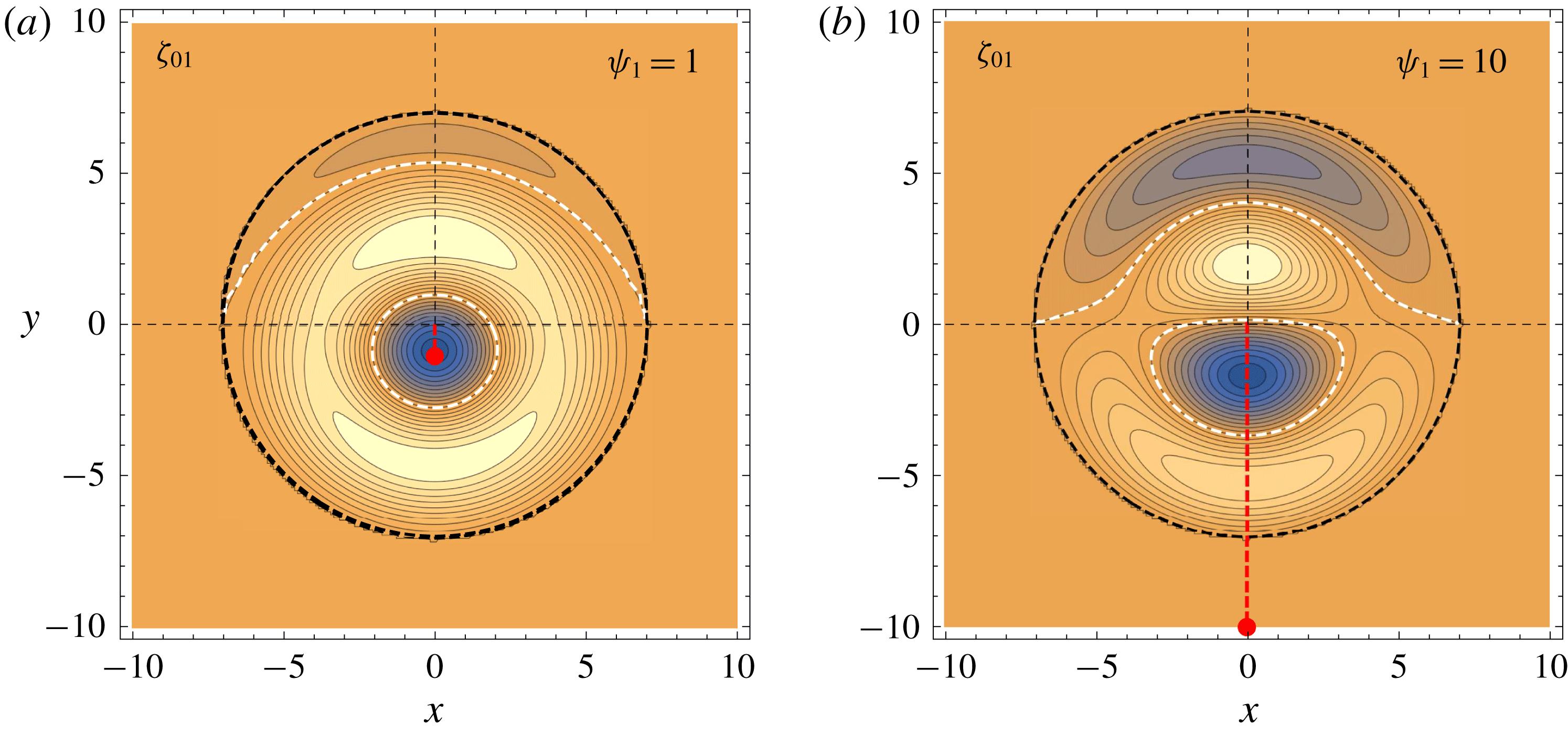
) implies changes of sign in the radial gradient of the mode-0 vorticity and the vortices are unstable. Examples of these solutions are plotted in figure 2 for different ratios
 $\unicode[STIX]{x1D713}_{1}/\unicode[STIX]{x1D713}_{0}$
and
 $n=2$
. For ratios
 $|\unicode[STIX]{x1D713}_{1}/\unicode[STIX]{x1D713}_{0}|$
smaller than the radius separating the inner and outer solutions
 $j_{1,2}\simeq 7.016$
(figure 2
a), the vortex resembles a single one-signed negative vorticity vortex with a positive small-amplitude vorticity perturbation that apparently rotates around the negative vortex centre at a rotation rate
 $\bar{\unicode[STIX]{x1D714}}_{0}$
depending only on
 $\unicode[STIX]{x1D713}_{0}$
(as well as on the number
 $n$
of vorticity shells), and is therefore independent of the mode-1 amplitude
 $\unicode[STIX]{x1D713}_{1}$
. Numerical simulations confirm this behaviour initially, though the vortices soon become unstable for
 $n\geqslant 2$
(an example is shown in Movie 3).
Vorticity
 $\unicode[STIX]{x1D701}_{01}$
for the mode-0+1 vortex with
 $n=2$
vorticity shells and amplitude ratios
 $\unicode[STIX]{x1D713}_{1}/\unicode[STIX]{x1D713}_{0}=1$
(a), and
 $\unicode[STIX]{x1D713}_{1}/\unicode[STIX]{x1D713}_{0}=10$
(b). Amplitude
 $\unicode[STIX]{x1D713}_{0}=1$
. Blue colours correspond to negative values. The black dashed circle separates the interior from the exterior solution. The white dashed line is the contour
 $\unicode[STIX]{x1D701}_{01}=0$
. The red dashed segment, with a length equal to
 $\unicode[STIX]{x1D713}_{1}/\unicode[STIX]{x1D713}_{0}=\unicode[STIX]{x1D713}_{1}$
, is the radius of the vortex trajectory.

These mode-0+1 vortex examples rotate with the same frequency
 $\bar{\unicode[STIX]{x1D714}}_{0}$
but along a circle with a radius given by
 $|\unicode[STIX]{x1D713}_{1}/\unicode[STIX]{x1D713}_{0}|$
(independent of
 $n$
). For
 $|\unicode[STIX]{x1D713}_{1}/\unicode[STIX]{x1D713}_{0}|=j_{1,1}$
, the radius coincides with the vortex radius. For larger ratios
 $|\unicode[STIX]{x1D713}_{1}/\unicode[STIX]{x1D713}_{0}|\gg j_{1,1}$
(figure 2
b), the vortex time evolution approaches the behaviour of a single dipole following a straight path, or infinite curvature radius as
 $\unicode[STIX]{x1D713}_{0}\rightarrow 0$
. The vorticity geometry of the C–L dipole remains unchanged enclosed in the first vorticity shell. When isolated (by setting
 $n=1$
) the particular C–L dipole displaces along a circle with the same radius
 $|\unicode[STIX]{x1D713}_{1}/\unicode[STIX]{x1D713}_{0}|$
, but different angular velocity
 $\bar{\unicode[STIX]{x1D714}}_{0}=\unicode[STIX]{x1D713}_{0}\text{J}_{0}(j_{1,1})/2$
, rotating in the opposite direction to the case
 $n=2$
.
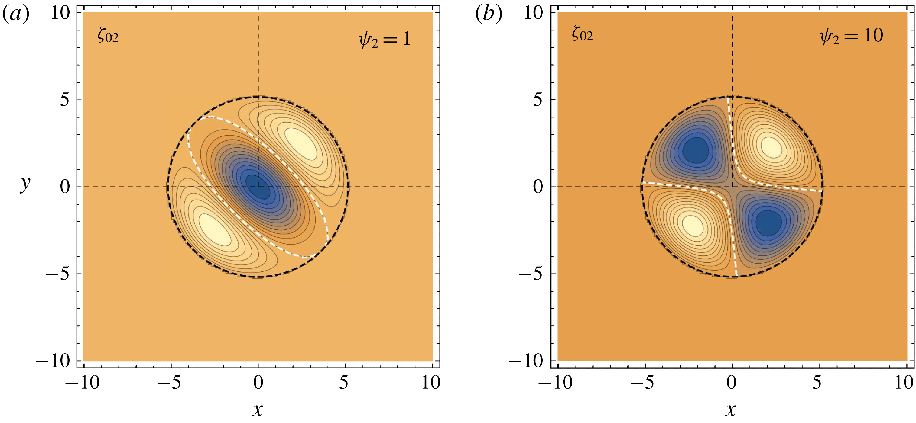
Vorticity field
 $\widetilde{\unicode[STIX]{x1D701}}_{02}(x,y,0)$
for the combination of mode-0 and mode-2 with amplitudes (a)
 $\hat{\unicode[STIX]{x1D713}}_{2}=\text{i}$
, and (b)
 $\hat{\unicode[STIX]{x1D713}}_{2}=10\text{i}$
. Amplitude
 $\unicode[STIX]{x1D713}_{0}=1$
. Blue colours correspond to negative values. The black dashed circle separates the interior from the exterior solution. The white dashed line is the contour
 $\widetilde{\unicode[STIX]{x1D701}}_{02}=0$
.

5 Concluding remarks
Multipolar vortices with azimuthal-mode dependence
 $\exp (\text{i}m\unicode[STIX]{x1D703})$
, and separation of polar and time variables
 $(r,\unicode[STIX]{x1D703},t)$
, are steady nonlinear solutions to the two-dimensional Euler equations whose radial dependence is given by the Bessel functions of the first kind
 $\text{J}_{m}(r)$
. These vortices have non-vanishing velocity at infinity. For modes
 $m=0$
and
 $m=1$
, the far flow field is a rigid velocity field, and unsteady vortex solutions, with vanishing velocity at infinity, can be explicitly found in terms of a reference frame change. The addition of modes 0 and 1 is a particular C–L dipole, with continuous vorticity, found to be stable through numerical simulations.
For azimuthal modes
 $m\geqslant 2$
, the far-field flow is no longer a rigid motion and the unsteady solutions involve vorticity field deformation. The important challenge is to find their time-dependent solutions with vanishing velocity at infinity. These modes are dispersive in the sense that their corresponding dipoles tend to move in different directions. As an example let us consider the vorticity distribution
 $\widetilde{\unicode[STIX]{x1D701}}_{02,1}(x,y,0)$
(figure 3) only as a vorticity field at a given time (
 $\widetilde{\unicode[STIX]{x1D701}}_{m,1}(x,y,t)$
are not solutions for
 $m\geqslant 2$
). For
 $\Vert \hat{\unicode[STIX]{x1D713}}_{2}\Vert /|\unicode[STIX]{x1D713}_{0}|\leqslant 1$
, the vortex resembles a rotating tripole (figure 3
a), while for
 $\Vert \hat{\unicode[STIX]{x1D713}}_{2}\Vert /|\unicode[STIX]{x1D713}_{0}|\gg 1$
, the two dipoles would tend to travel in opposite directions along the
 $x$
-axis, (figure 3
b).
Numerical simulations, using a pseudo-spectral code and initial vorticity conditions
 $$\begin{eqnarray}\unicode[STIX]{x1D701}_{02}(\unicode[STIX]{x1D712})=\unicode[STIX]{x1D701}_{0}[\text{J}_{0}(\unicode[STIX]{x1D712})-\text{J}_{0}(j_{1,1})]+\unicode[STIX]{x1D701}_{2}\text{J}_{2}\left(\unicode[STIX]{x1D712}\frac{j_{2,1}}{j_{1,1}}\right)\sin (2\unicode[STIX]{x1D703}),\quad \unicode[STIX]{x1D712}\leqslant j_{1,1},\end{eqnarray}$$
where the radial dependence in the second mode is scaled by
 $j_{2,1}/j_{1,1}$
to match
 $\unicode[STIX]{x1D701}_{02}(j_{1,1})=0$
, show that, simplifying the results description, the vortex (5.1) presents three different main evolution regimes depending on the initial amplitude ratio. When mode-0 dominates mode-2 (initial amplitude ratio
 $|\unicode[STIX]{x1D701}_{2}|/|\unicode[STIX]{x1D701}_{0}|\ll 1$
), the mode-2 vorticity anomalies are circularly advected by the dominant mode-0 flow inside the vortex and, since these are vorticity anomalies of both signs, form a spiral pattern whose radial wavenumber increases with time inside the vortex (Rhines & Young Reference Rhines and Young1983) until their amplitude is reduced by numerical dissipation when their radial wavelength approaches the grid size. In the case of both modes having amplitudes of the same order, the vortex evolves towards a tripole, with one central vortex and two satellite vortices of opposite vorticity sign. When mode-2 dominates mode-0 (
 $|\unicode[STIX]{x1D701}_{2}|/|\unicode[STIX]{x1D701}_{0}|\gg 1$
), the two dipoles move initially in opposite directions – in this case the mode-0 vorticity anomalies being advected by the dominant mode-2 flow. Due to the non-axisymmetric vorticity anomaly distribution caused by the mode-0 amplitude
 $\unicode[STIX]{x1D701}_{0}$
, the dipoles describe two curved trajectories, with opposite signed curvatures, as if they were two stable modified C–L dipoles with mode-0 amplitudes
 $\pm \unicode[STIX]{x1D701}_{0}$
.
Acknowledgements
I thank three anonymous referees for their very helpful comments. Partial support for this study was obtained through project CTM2014-56987-P (Spanish Ministry of Science and Innovation).
Supplementary movies
Supplementary movies are available at https://doi.org/10.1017/jfm.2018.892.
Appendix A. Azimuthal-mode solutions
The material conservation of vorticity (2.2) applied to stream functions with azimuthal-mode dependence and separation of polar and time variables
 $(r,\unicode[STIX]{x1D703},t)$
in the form
 $$\begin{eqnarray}\unicode[STIX]{x1D6F9}(r,\unicode[STIX]{x1D703},t)=\unicode[STIX]{x1D713}(r)\text{e}^{\text{i}m\unicode[STIX]{x1D703}}T(t),\end{eqnarray}$$
leads to
 $$\begin{eqnarray}m\frac{\unicode[STIX]{x1D713}(r)}{r}\left[\frac{\left(\unicode[STIX]{x1D713}^{\prime \prime }+{\displaystyle \frac{\unicode[STIX]{x1D713}^{\prime }}{r}}-m^{2}{\displaystyle \frac{\unicode[STIX]{x1D713}}{r^{2}}}\right)^{\prime }}{\unicode[STIX]{x1D713}^{\prime \prime }+{\displaystyle \frac{\unicode[STIX]{x1D713}^{\prime }}{r}}-m^{2}{\displaystyle \frac{\unicode[STIX]{x1D713}}{r^{2}}}}-{\displaystyle \frac{\unicode[STIX]{x1D713}^{\prime }}{\unicode[STIX]{x1D713}}}\right]=-\frac{T^{\prime }(t)}{T^{2}(t)}\text{i}\text{e}^{-\text{i}m\unicode[STIX]{x1D703}}.\end{eqnarray}$$
For
 $m\neq 0$
, the term on the left-hand side of (A 2) depends only on
 $r$
, but the term on the right-hand side has an explicit dependence on
 $\unicode[STIX]{x1D703}$
, hence
 $T^{\prime }(t)=0$
, and the flow is steady. For
 $m=0$
,
 $T^{\prime }(t)=0$
follows directly. Thus, for
 $m=0$
any, well-behaved, radial function
 $\unicode[STIX]{x1D713}(r)$
is a steady solution. For
 $m\neq 0$
(A 2) implies
 $$\begin{eqnarray}\left(\log \frac{\unicode[STIX]{x1D713}^{\prime \prime }+{\displaystyle \frac{\unicode[STIX]{x1D713}^{\prime }}{r}}-m^{2}{\displaystyle \frac{\unicode[STIX]{x1D713}}{r^{2}}}}{\unicode[STIX]{x1D713}}\right)^{\prime }=0,\end{eqnarray}$$
which reduces to the Bessel differential equation
 $$\begin{eqnarray}r^{2}\unicode[STIX]{x1D713}^{\prime \prime }(r)+r\unicode[STIX]{x1D713}^{\prime }(r)+(c_{0}^{2}r^{2}-m^{2})\unicode[STIX]{x1D713}(r)=0.\end{eqnarray}$$
Setting
 $c_{0}=1$
in (A 4) is equivalent to choosing the integration constant in (A 3) equal to
 $\text{i}\unicode[STIX]{x03C0}$
.