

1. Introduction
In 1992, researchers at the World Bank profiled how six environmental problems, ranging from carbon dioxide emissions to the percentage of the population without access to safe drinking water, respond to changes in per capita income. They described three distinct patterns: some environmental problems worsened as per capita income increased (municipal wastes per capita and carbon dioxide emissions per capita); some improved along with per capita income (the percentage of the population without safe water or adequate sanitation, and concentrations of airborne particulate matter); and some initially worsened and then eventually began to improve (concentrations of sulfur dioxide) (World Bank, 1992).
Curiously, it is the latter which has most captured the attention of many economists and policy makers. The ‘inverted-U’ described by the trajectory of sulfur dioxide concentrations against per capita income – called the ‘environmental Kuznets curve’ due to its similarity to the theoretical relationship between per capita income and inequality – has been used incautiously by some to conclude that ‘in the end the best – and probably the only – way to attain a decent environment . . . is to become rich’ (Beckerman, Reference Beckerman1992).
Tempting as it may be to arrive at this conclusion, it would be unwise for several reasons. First, as the World Bank found, the phenomena that fall into the ‘inverted-U’ category represent only a subset of environmental problems. Second, as Arrow et al. (Reference Arrow, Bolin, Costanza, Dasgupta, Folke, Holling, Jansson, Levin and Mäler1995) point out, the inverted-U does not ‘constitute evidence that it [the decline of pollution] will. . .happen in time to avert the important and irreversible global consequences of growth’. Third, as Grossman and Krueger (Reference Grossman and Krueger1995) state, there is nothing automatic about relationships that have proven true – in some places – in the past. While pollution levels may have declined after a turning point in some developed countries as per capita income grew, this does not necessarily imply that the same can or will occur in developing countries. For these reasons, one must consider the underlying reasons behind such a curve, where it exists.
The literature on the environmental Kuznets curve to date is vast and constantly evolving. It covers a wide variety of pollutants (air, water, and land) as well as other types of environmental damages, such as deforestation (Ehrhardt-Martinez et al., Reference Ehrhardt-Martinez, Crenshaw and Jenkins2002). Explanatory variables have been expanded to include the sectoral composition of GDP (Panayotou, Reference Panayotou1997), trade (Antweiler et al., Reference Antweiler, Copeland and Taylor2001), energy input (Stern, Reference Stern2002), democracy (Deacon, Reference Deacon1999; Barrett and Graddy, Reference Barrett and Graddy2000), civil liberties and inequality (Torras and Boyce, Reference Torras and Boyce1998), and others, all in an effort to explain the negative relationship between income and pollution observed at high levels of income. Finally, more recent work has challenged the very existence of an EKC, pointing to the use of inappropriate statistical techniques in some of the earlier literature (Perman and Stern, Reference Perman and Stern2003).
However, as Grossman and Krueger (Reference Grossman and Krueger1995) point out, the introduction of such explanatory variables as those listed above complicates the picture. Their paper uses a reduced-form equation linking per capita income and pollution. A reduced-form equation has the advantage of simplicity: it indicates the ‘net’ effect of income growth on pollution. The alternative to a reduced-form equation, Grossman and Krueger (Reference Grossman and Krueger1995) point out, is to estimate a series of structural equations. To find the net effect of income on pollution would require ‘solving back’ to find it, and the introduction of other explanatory variables, many of which are of questionable precision, could potentially introduce bias into the estimates.
A drawback of the reduced-form equation is that it does not indicate the specific causal mechanism at work. It is impossible, using a reduced-form equation, to distinguish between the changes within a country accompanying economic growth resulting in an increase in pollution from those resulting in a decrease in pollution. However, it is possible to disaggregate short-term income fluctuations from the trend of income growth over time. The former would likely result in temporary increases or decreases in pollution, depending on whether short-term income had increased or decreased and how the economy responds in the short term; the latter, encompassing long-term changes in the sectoral composition of the economy and the technologies used in production, is ambiguous, depending on the specific sectoral change and whether new technologies are more or less polluting. This paper modifies Grossman and Krueger's (Reference Grossman and Krueger1995) original specification in a way that allows for better isolation of short-term versus long-term income changes.
Section 2 summarizes the relevant literature. To do a comprehensive summary of the ever-evolving EKC literature is beyond the scope of this paper; the interested reader is directed to Stern (Reference Stern2003). Section 3 presents the econometric model used. Section 4 discusses the data, section 5 presents the results, and section 6 concludes.
2. The scale, composition, and technology effects
2.1. Long-run changes in income
The scale effect arises from the simple fact that economies with higher per capita incomes both produce and consume more goods and services. Holding output mix and production techniques constant, an increase in scale necessarily brings about a proportionate increase in pollution. As Stern (Reference Stern2002) explains, ‘if there were no growth in the structure or technology of the economy, pure growth in the scale of the economy would result in a proportional growth in pollution and other environmental impacts’. Generally, however, as long-run per capita income grows, both the output mix and available technologies change. Depending on the direction of these changes, a given unit of income may be associated with less or more pollution.
In the industrialized countries, economic growth has been accompanied by a shift in production patterns from the more material- and energy-intensive manufacturing sector toward the (theoretically) more environmentally friendly service sector (Jayadevappa and Chhatre, Reference Jayadevappa and Chhatre2000). Consumption patterns have shifted as well, yet whether consumption patterns of the wealthy are more or less polluting than those of the poor depends on the contaminant in question. In addition, international trade permits a country's production patterns to diverge from its consumption patterns, as its citizens consume goods produced in other countries and produce goods consumed elsewhere (Copeland and Taylor, Reference Copeland and Taylor1997). All can contribute to the ‘composition effect’ of rising per capita incomes.
The technology effect (referring to changes in the state of technological development) allows for the possibility that, as countries develop, new technologies are developed that increase total factor productivity. The technology effect can be separated into two elements. One is the ‘autonomous’ technology effect, in which the development of cleaner processes occurs more or less exogenously through increases in scientific and technological knowledge. As a result, pollution per unit of output could decline while holding the output mix constant, although decreases in pollution may not be the intended result of such technological advances.
The other element of the technology effect is the ‘induced’ technology response, which is brought about by changes in the relative price of factors (Hicks, Reference Hicks1939). The induced technology response may include what this paper terms the ‘politically induced technology response’, whereby demand for a cleaner environment is translated into public and private decisions to cut pollution (Heerink et al., Reference Heerink, Mulatu and Bulte2001). Demand for environmental quality has been widely documented to be a ‘normal’ good (see, for example, Copeland and Taylor, Reference Copeland and Taylor2004). The implementation of the Clean Air Act in the United States, for example, was in part a response to the growing demand for cleaner air. Technological change in response to regulatory mandates, such as compulsory installation of end-of-pipe scrubbers in stacks to reduce sulfur dioxide emissions, is an example of such a response. The induced policy response in part therefore reflects consumers' demand for cleaner production processes. The possibility of such politically induced technology responses suggests that an important intervening variable in the income per capita−pollution relation may be the extent of democracy (such that demand for environmental quality is politically effective). Many other studies (Torras and Boyce, Reference Torras and Boyce1998; Deacon, Reference Deacon1999; Barrett and Graddy, Reference Barrett and Graddy2000) have found negative relationships between political rights and civil liberties and the concentrations of certain air pollutants. If the technology effect (both exogenous and induced) were sufficiently strong, total pollution could decline even as output rises.
To advance our understanding of the relationship between environmental degradation and per capita income, it would be useful to be able to distinguish empirically among the long-term scale, composition, and technology effects, and to assess their relative strength. If, for example, the long-term scale effect is outweighed by pollution-reducing composition and/or technology effects, total pollution will fall with rising income over time. Previous studies have attempted to distinguish between the scale, composition, and technology effects by introducing new variables. Panayotou (Reference Panayotou1997), for example, defines scale as GDP per square kilometer, and composition by industry share of output. A variable measuring the respect for or enforcement of contracts is used as a proxy for the policy-induced technology effect. Stern (Reference Stern2002) approximates the composition effect by including variables measuring the value-added shares of agriculture, manufacturing, and other sectors as determinants of pollution; as a proxy for the technology effect he uses the ratio of GDP to total energy inputs. Once these are included, he treats the estimated coefficient on per capita income as a measure of the scale effect. Balsdon (Reference Balsdon2003) interacts measures of the degree of democracy with per capita income to assess the technology effect, reasoning that ‘“abatement” (technique) effects are fundamentally interacted with government in a way that “gross emissions” (or scale) are not, leading to an econometric specification capable of identifying them separately’. However, he does not attempt to identify the composition effect. While this study does not differentiate between the composition and technology effects, section 3 shows the possibility of distinguishing the long-term scale effect from the combined composition and technology effects.
2.2. Short-run fluctuations in income
Much of the literature to date has estimated the scale effect by using per capita GDP as a proxy. This approach has two limitations: one, that GDP per capita does not increase monotonically but is subject to fluctuations in the business cycle, and, two, that GDP per capita may be a non-stationary time series (Perman and Stern, Reference Perman and Stern2003). The first limitation will be discussed in this section; the second will be postponed to section 3. By not distinguishing changes in income arising through trends in the composition of output or advances in the state of technology from the short-term changes in income arising from temporary ‘booms’ and ‘busts’, the literature to date has assumed a number of things: income fluctuations have the same effect on pollution as income trends; pollution responds the same to booms as it does to busts; and no temporary adjustments in production processes, such as changes in fuel mix, take place. There are several reasons to question these assumptions.
The neoclassical theory of the firm introduces the notion of a ‘shutdown point’, a price below which a firm shuts down rather than continuing to operate. This theory implies that during periods of recession, a polluting firm in the steel industry, for example, would shut its furnaces down rather than continue to operate them. In actuality, steel furnaces are typically operated at low output rates, rather than shutting them down and having to restart them later (Klein and Robison, Reference Klein and Robison1992). Energy efficiency is very low during those times, implying that pollution might have a ‘fixed’ and a ‘variable’ component. During recessionary times, therefore, pollution might not decrease by the same percentage as output. Firms may also use a different fuel mix during times of low or high output demand, thus polluting either proportionately more or less than during non-recessionary, non-boom times. In addition, anecdotal evidence suggests that firms in the pulp and paper industry in Maine consistently operate below their regulatory license limits, so that a boom in activity or an upset in pollution control technology may not result in exceeding pollution control limits. As firms simply take advantage of previously idle capacity, then, a temporary increase in economic activity may not result in a proportionate increase in pollution.
Some sectors of the economy may be more susceptible to short-term booms and busts as well. Although there is evidence of high industry co-movement, some sectors of the economy may be more sensitive than others to upturns or downturns in the economy (Hornstein, Reference Hornstein2000). Depending upon how ‘dirty’ (‘clean’) these sectors are, a 1 per cent increase in economic activity during a boom might result in a more than (less than) 1 per cent increase in pollution in the short term. That does not imply that the sectoral composition of the economy has changed in any permanent or long-term manner.
A final reason why there may not be short-run constant returns to scale in production is that regulators may not be as vigilant during recessionary times. Deily and Gray (Reference Deily and Gray1991), for example, found evidence that regulators did not inspect firms experiencing tough economic times as frequently as they did other firms, indicating that regulators may take economic factors into consideration when inspecting a plant. Israel (Reference Israel2004) also found that regulation and enforcement may be relaxed during recessions.
Whatever the underlying reason, it is not necessarily the case that an increase in output during an upward swing in the business cycle would have the same effect on emissions as an increase in permanent income. By not distinguishing between the permanent ‘trend’ of income, and the temporary ‘fluctuations’ of income, EKC models using per capita GDP as a proxy for the scale effect are conflating short-term ‘noise’ with long-term trends, introducing distortion into the results. Making the distinction between short-term income fluctuations and the trend of income over time allows us to distinguish the effects of changes in the scale of the economy over time from short-term fluctuations in production, resulting from a recession or a boom.
This paper relies on data for sulfur dioxide (SO2) emissions to test this hypothesis. Sulfur dioxide is a colorless gas with a pungent odor. It is formed when fuels containing sulfur (mainly coal and oil) are burned and during various industrial processes, such as smelting. Short-term exposure to high levels of sulfur dioxide can be life-threatening. Long-term exposure to atmospheric sulfur dioxide can lead to or exacerbate asthma and other respiratory illnesses, and aggravate existing heart disease (Environmental Protection Agency, 2008). In addition, sulfur dioxide is a precursor to acid rain, which leads to the corrosion of buildings, monuments, and other structures, and has adverse impacts on forests and aquatic ecosystems.
The reasons for using SO2 emissions are four-fold. First, the purported inverted-U shape of the EKC has been found most consistently in studies using SO2 data. Second, data for SO2 emissions are widely available. Third, since SO2 is primarily associated with industrial production, using SO2 emissions allows us to focus primarily on industrial production. While it is possible that consumption as well as production contributes to SO2concentrations, emissions data reflect industrial sources of SO2, rendering estimates of changes in a country's consumption patterns unnecessary.
The next section will estimate a standard, reduced form EKC, regressing pollution per capita on per capita income, per capita income squared, and population density. Next, growth in per capita income will be decomposed into its ‘trend’ income and fluctuations around that trend. The two models will then be compared.
3. The ‘traditional’ versus ‘disaggregated’ EKC model
3.1. The traditional EKC model
The traditional EKC model, as first estimated by Grossman and Krueger (Reference Grossman and Krueger1995), is a reduced form equation, with some measure of per capita environmental degradation as the regressor and per capita income in some form as the regressands. This study follows the standard convention by using (Polit), the observed level of per capita emissions in country i at time t, as the dependent variable, and a quadratic or cubic form of logged per capita income (Yit), the observed income in country i at time t, as the independent variable.
Many studies of the income–degradation relationship have used ambient concentrations, rather than emissions, as the dependent variable. Both measures have advantages and drawbacks. If the goal is to study how environmental quality changes with economic growth, then ambient concentrations are a preferable measure for localized pollutants. However, ambient concentrations are affected by geographical variables such as topography, climate, and wind. For example, the existence of hills or thermal inversions may limit dispersion of contaminants. Ambient concentrations vary from place to place within any given country, rendering determining the appropriate measure for national-level analysis problematic. In addition, there is the issue of the spatial separation between emissions and concentrations: ‘Using emissions neither “punishes” countries that import pollution from areas over which they have little political control nor ‘rewards’ those that export pollution via prevailing winds’ (Scruggs, Reference Scruggs1998). Therefore, this paper employs data on emissions, rather than concentrations, of sulfur dioxide.
The ‘traditional’ EKC model estimated in this paper is

where Polit is the per capita emissions level, measured in metric tons; Yit is GDP per capita, corrected for purchasing power parity and measured in terms of thousands of 1987 international dollars per person; Popit/km 2 is population per kilometer squared; IDi is a country-specific dummy variable; YRt is a linear time trend; μ it is the error term, whose properties will be discussed below; I is the number of countries; the βs are the parameters to be estimated; and the subscripts i and t refer to the country and year, respectively.
Equation (1) illustrates a fixed-effects model, implying that all coefficients can be interpreted as the effect of differences from the mean of the independent variable on the dependent variable. As the level of income, for example, is estimated at the individual country level, the coefficient on income can be interpreted as the effect of the difference of the predicted level of GDP from the average level of GDP in a country over time.
The elasticity of emissions with respect to income, ɛey, is estimated either by

or

depending on whether the quadratic or the cubic specification is used.
Next, the model disaggregating income into the ‘trend’ of income and the fluctuations around that trend is estimated. The two models will then be compared, to determine if the elasticity of emissions with respect to income is substantially different between the two models.
3.2. A disaggregated model of the income–degradation relationship
I begin by estimating separately the environmental impact of the trend in GDP and that of fluctuations around that trend. The composition and policy-induced technology effects are assumed to operate only through the trend of income over time: they are expected to affect the income–degradation relation gradually, with little sensitivity to year-to-year income fluctuations. Fluctuations of income, however, are expected to have a different effect on pollution, as explained in section 2. These short-run variations in GDP, unlike long-run growth, are not expected to alter substantially either the long-run composition of output or the state of technology. Fosler and Stiroh (Reference Fosler and Stiroh1998), for example, demonstrate that business cycle fluctuations, while certainly affecting the short-run output of individual sectors of the economy, do not affect significantly the aggregate composition of output.
Other studies have attempted to proxy permanent income by including some version of lagged per capita GDP. For example, Grossman and Krueger (Reference Grossman and Krueger1995) use an average of the GDP from the three preceding years. This specification does not adequately capture the trend of income over time, however. First, a three-year average is not a long enough time to reflect changes in the underlying structure of an economy. Second, one year of abnormal positive or negative growth could significantly skew the three-year average. Using an average over a longer period of years, though, may render some observations without a long time series unusable. By regressing income over time, all the data at our disposal may be used to construct a more accurate trend. Thus, the effects of a long-term trend in income, reflecting the scale, composition, and induced technology effects, can be more cleanly separated from short-term changes in income that deviate from that trend.
Decomposing income into fluctuations and trend, we can obtain two independent variables: Yit*, the trend level of income, and (Yit − Yit*), the fluctuations around that trend. The income trend variable is obtained by regressing the log of per capita GDP on the year and year squared, and obtaining the fitted values. The following regression was performed for each country

where Yt is the observed level of income at year t and Yrt and Yrt 2 are the year and year squared respectively and μt is the error term. The fitted values, Yi*, are used as the measure of trend level of income in equation (5) below. The residuals of equation (4) are used as the measure of fluctuation around the trend. This exercise was repeated for each country in the sample, as requiring all countries in the sample to have a common trend clearly is overly restrictive. In other words, the ‘trend’ variable and the fluctuations are country specific. Various specifications were tested; a quadratic function of year ultimately was chosen because tests of the residuals found no systematic pattern.
Given this theory, the following estimation will be used

where Polit is the per capita emissions level, measured in metric tons; Yit* is the trend value of income, as defined above; Yit is the actual value of per capita GDP; Popit/km 2 is population per kilometer squared; IDi is a country-specific dummy variable; YRt is a linear time trend; μ it is the error term, whose properties will be discussed below; I is the number of countries; the ηs are the parameters to be estimated; and the subscripts i and t refer to the country and year, respectively.
Equation (5) implies that the pollution level can be explained by the trend in income, and the fluctuations around that trend. Both a quadratic specification and a cubic specification are used for income, as some studies (e.g., Grossman and Krueger, Reference Grossman and Krueger1995) have found evidence of an upward swing in pollution at very high income levels.
The interpretation of the coefficient of the fluctuations variable (the residuals of equation (4)) is straightforward, as the mean of the residuals is zero.
The elasticity of emissions with respect to the trend level of income, ɛey*, is estimated either by

or

depending on whether the quadratic or the cubic specification is used.
The trend level of income represents the trend of a country's per capita GDP over time, relative to the average level of income. This combines the effects of the scale of the economy, the sectoral composition of the economy, and any policy-induced changes in technology. The elasticity of pollution with respect to the trend level of income therefore captures these combined effects. The fluctuations around the trend, Yit – Yit*, capture only the effects of short-term increases or decreases in per capita GDP, assuming the combined effects of the long-term sectoral composition and policy-induced technological change remain constant. The elasticity of pollution with respect to income fluctuations is measured as a constant elasticity by the coefficient η 4.
We are interested in disaggregating the effects of the scale from the effects of the combined sectoral composition and policy-induced technological development. We can isolate the combined effects of sectoral composition and technological change by subtracting the elasticity of pollution arising from the scale effect from the elasticity of pollution with respect to the trend level of income. By definition, the scale effect is the result of increasing the output of the economy while holding the sectoral composition of production and technological change constant. Therefore, the elasticity of emissions with respect to the scale effect is assumed to be unitary, allowing us to find the combined effects of sectoral composition and policy-induced technological change by subtracting 1 from the elasticity of pollution with respect to the trend level of income. A negative value indicates that a stronger combined composition and induced technology effect would tend to decrease emissions; a positive value indicates the opposite.
Finally, a linear time trend is included to capture any changes in technology or preferences that are unrelated to income levels.
3.3. Hypotheses
The coefficient on income fluctuations can be interpreted as the effect of a temporary increase or decrease in output. If pollution exhibited short-run constant returns to scale in production, the elasticity of emissions with respect to income fluctuations would be 1.0. It may be the case that emissions comprise both a fixed component that is more or less inelastic with respect to income fluctuations and a variable component with approximately unit elasticity. If so, the estimated elasticity (which can be read directly from the coefficient in this specification since both variables are in natural logarithms) would be between zero and one. Theoretically, pollution could decrease even while the economy is experiencing a temporary increase in activity, through short-term changes in the composition of output or production processes. Therefore, the elasticity of emissions with respect to income fluctuations may be either positive or negative. Likewise, the elasticity of emissions with respect to the trend of income over time may be positive or negative – positive if the scale effect outweighs the combined composition and technology effect; negative if the opposite is true.
The hypothesized signs of the remaining coefficients are as follows. The expected sign on the population coefficient is uncertain, as, on the one hand, higher population density may imply higher emissions due to urbanization, while, on the other hand, countries with higher population densities may be more concerned about abating emissions (Panayotou, Reference Panayotou1997). The coefficient on the linear time trend is expected to be negative, as it captures any changes in technology and preferences exogenous to income. Finally, the elasticity of emissions with respect to income in the traditional estimation is hypothesized to be larger in magnitude than the elasticity of emissions with respect to the trend level of income in the disaggregate model. Once income fluctuations are controlled for, emissions are hypothesized to be less responsive to changes in the trend level of income.
3.4. Issues in estimation
Equations (1) and (5) are estimated by a fixed-effects method. Each country is assumed to have its own intercept, while the slope coefficients are common to all countries. A Hausman test indicated that a fixed effects model was preferable to a random effects model, as evidence was found of correlation between the cross-sectional error term and the other regressors. A log-ratio test was used to test for heteroskedasticity across panels: the model was estimated with and without correcting for panel-level heteroskedasticity, and their log ratios then compared. Evidence was found for panel-level heteroskedasticity. Evidence was also found for first-order serial autocorrelation, using a Durbin−Watson test on each of the individual countries. The Huber/White method of determining standard errors (sometimes called the sandwich estimator of variance) was therefore used to adjust for the various issues that arose in estimation (Stata Corp, 2001).
A further complication is that equation (5), the model that disaggregates income into its trend and fluctuations, has non-stochastic regressors, due to the inclusion of both the predicted value of income and the residuals from equation (4).Footnote 1 The standard errors were thus adjusted using a method reported in Murphy and Topel (Reference Murphy and Topel1985), whereby the standard errors for the predicted variables were inflated by a common factor, using information from both the first-stage and the second-stage regressions.
A recent debate within the environmental Kuznets curve literature concerns whether the two time series of pollution and per capita income can be characterized as random walks; in other words, whether the level in time t can be expressed as a function of the level in time t–1, plus a random error (Perman and Stern, Reference Perman and Stern2003). If such were the case, then performing a regression with the two time series may bring about spurious results. As the average time series used in this study is 13 years (a relatively short time series), this is unlikely to be a problem. Furthermore, using a test developed by Levin et al. (Reference Levin, Lin and Chu2002), the null hypothesis of non-stationarity was rejected for all countries in the sample. As for per capita income, the null hypothesis of non-stationarity was rejected after a trend term was removed, indicating that, at least for this sample of countries and years, per capita income can be modeled as a stationary variable around a deterministic time trend.
4. Data
Data on sulfur dioxide emissions were obtained from the United Nations Economic Commission for Europe and the Co-operative Program for Monitoring and Evaluation of the Long-Range Transmission of Pollutants in Europe, as reported to the World Resources Institute's Earth Information Portal (World Resources Institute, 2005).Footnote 2 Emissions are divided by the population of the country, obtained from the World Development Indicators (World Bank, 2003) to obtain per capita emissions. Data on the per capita level of GDP, adjusted for purchasing power parity, come from the World Resources Institute's (2005) Earth Information Portal.
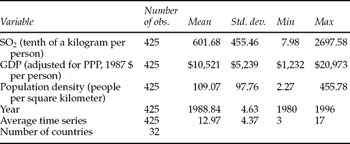
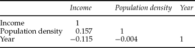
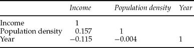
Summary statistics and correlation coefficients for all variables are reported in tables 1 and 2, respectively. The available data include European countries, Canada, and the United States – all countries that reported their emissions to the Economic Commission for Europe. The countries' per capita incomes (in 1987 PPP–adjusted dollars) range from $1,232 to $20,973. Hence, one should be cautious about extrapolating the results to other countries. Sulfur dioxide emissions per capita vary widely, from a low of 0.798 kg per person (Armenia in 1995), to 269.76 kg per person (Bulgaria in 1987). The average time series is 12.97 years, with the shortest time series being three years, and the longest series 17 years.
Descriptive statistics

Correlation coefficients (traditional model)
5. Results
5.1. Traditional model
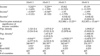
Results for the traditional model (that is, with the income variable measured simply as per capita GDP) are reported in table 3. All models are statistically significant at the 0.01 per cent level. The coefficients on the income and income squared terms describe an inverted-U relationship. The addition of a cubic term renders the income variables statistically insignificant individually, but an F-test showed them to be jointly statistically significant. Using model 1, the turning point occurs at $18,010 in 1987 PPP-adjusted dollars, a level of income roughly equivalent to that of Canada in the late 1980s, at the high end of the sample. However, the standard errors of the turning point, calculated by the delta method,Footnote 3 indicate the possibility of no turning point within the sample, as the upper end of a 90 per cent confidence interval around the estimate is outside of the sample. When graphed at the mean level of the variables, the graph shows a monotonically increasing relationship, with no visible turning point within the sample. Results for the model using a cubic function in income are similar. (The turning points and graph are available upon request.)
Effect of income on sulfur dioxide emissions, ‘traditional’ model
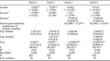
Notes: Huber/White standard errors. ***statistically significant at the 10% level, **statistically significant at the 1% level, *statistically significant at the 0.1% level.
Other comparable studies have found widely differing turning points. Selden and Song (Reference Selden and Song1994) found an estimated turning point of $10,391–$10,620 (constant 1985 US dollars) in their sample of 22 OECD and eight developing countries (although they do not include standard errors of the estimates). Cole et al. (Reference Cole, Raynor and Bates1997), using a dataset of 11 OECD countries, found a turning point of $5,700–$6,900, also in constant 1985 US dollars. Their reported standard errors are relatively small. Stern and Common (Reference Stern and Common2001), using a much larger dataset of emissions in 73 developing and developed countries, actually found a turning point of $101,116 in PPP-adjusted GDP.
Studies that have used sulfur dioxide concentrations (which are usually associated with lower turning points than those using ambient concentrations), such as Shafik (Reference Shafik1994), who found a turning point of $3,674 in PPP adjusted GDP, Torras and Boyce (Reference Torras and Boyce1998), who reported a turning point of $3,890, also in PPP-adjusted GDP, and Kaufman et al. (Reference Kaufmann, Davidsdottir, Garnham and Pauly1998), who estimated a turning point of $12,500 in 1985 US dollars. None of these results includes standard errors around the estimated turning point.
Using model 1, the elasticity of sulfur dioxide emissions with respect to income at the mean is approximately 0.379, indicating that a 10 per cent increase in per capita income is associated with a nearly 3.8 per cent increase in sulfur dioxide emissions. However, the elasticity differs at high and low levels of income. At low levels of income (levels corresponding to that of Poland or Bulgaria in the early 1990s, for example), the estimated elasticity of emissions with respect to income is greater than one, indicating that a 1 per cent increase in income may be associated with a greater than 1 per cent increase in sulfur dioxide emissions. Recall that this specification does not control for changes in the sectoral composition of the economy or in the technology used, so this result is perfectly plausible. At high levels of income (levels corresponding to that of Switzerland or the United States), the point estimate elasticity of emissions with respect to per capita income turns negative, indicating that a 1 per cent increase in income may be associated with a decrease in emissions. However, the latter results are not statistically different from zero, indicating that the combined ‘composition’ and ‘technology’ effects may equal or possibly exceed the scale effect at high levels of income. (These results are available upon request.)
The estimated coefficient on population density is positive, indicating that the more densely populated a country, the higher its level of per capita sulfur dioxide emissions. The result is only statistically significant when a quadratic of the variable is included, indicating that the result is non-linear. Finally, the estimated coefficient on the linear time trend indicates that sulfur dioxide emissions have been declining over the years in the sample, due to autonomous changes in technology or other changes not related to income.
5.2. Disaggregated model
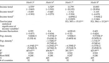
Results of the disaggregated model are shown in table 4. At first glance, the results seem to be similar to the traditional model. All the models are statistically significant at the 0.01 level. There is an indication of an inverted-U in emissions, as the estimated coefficient on the trend level of income is positive, and the estimated coefficient on its square is negative. As with the traditional specification, the addition of a cubic term renders the income variables statistically insignificant individually, but an F-test showed them to be jointly statistically significant.Footnote 4 The estimated ‘turning point’, using model 5, occurs at approximately $15,000, the per capita trend level of income of France in the late 1980s.Footnote 5 The ‘turning points’ between this model and the traditional model cannot be directly compared, as the turning point in the traditional model is in per capita income terms, while the turning point in the disaggregated model is in trend income terms. However, in the late 1980s, France's per capita level of income was about $15,600, implying that the turning point in the disaggregated model occurred at a lower level of income than in the traditional model ($18,010). A 90 per cent confidence interval around the estimate shows that we cannot reject the hypothesis that the two turning points may be the same, nor can we reject the possibility that the turning point lies outside of the sample. A graph of emissions per capita with respect to per capita income, with population density and the year at their respective mean values, shows a curve with a turning point near the end of the sample. (The turning points and graph are available upon request.)
Effect of income on sulfur dioxide emissions, disaggregated model
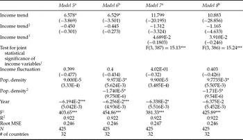
Notes: Huber/White standard errors. ***statistically significant at the 0.1% level, **statistically significant at the 1% level, *statistically significant at the 10% level.
astandard errors for income variables inflated by a factor of 2.01.
bstandard errors for income variables inflated by a factor of 1.84.
†F-statistics are approximate. See footnote 4 in text.
At the mean level of trend income, the estimated elasticity of emissions using model 5 is about 0.32, lower than the estimated elasticity with respect to income in the traditional model as hypothesized, but not statistically significantly different. The same results regarding elasticity at different levels of income hold true here: at low levels of trend income, the elasticity of emissions with respect to trend income is positive; at very high levels of trend income, the elasticity of emissions with respect to trend income turns negative, although not statistically different from zero, implying that emissions may not change with increased levels of per capita income. These results are broadly consistent with those from the traditional model.
The estimated coefficient on the fluctuations of income around the trend in model 5 is 0.41 but not statistically significant at conventional levels, indicating that a 1 per cent positive fluctuation in income is associated with a 0.41 per cent increase in emissions. Since the elasticity of emissions with respect to short-term fluctuations is less than 1, there may be a significant ‘fixed’ component of pollution.
Recall that by disaggregating the trend in income from the fluctuations in income, it may be possible to distinguish the long-run scale effect from the long-run composition and technology effects. The estimated elasticity with respect to the trend level of income reflects the long-run scale, composition, and technology effects together; the elasticity with respect to the long-run scale effect is unitary, by definition. Therefore, subtracting 1 from the former (ɛey* − 1) should give us an idea of the sign of the combined composition and technology effects.
Performing this calculation at the mean level of income yields −0.68, implying that, at the mean level of income, the combined composition and policy-induced technology effects contribute negatively to emissions. At very low levels of income in the sample the combined composition and technology effects contribute positively to emissions. These results are available upon request.
The negative and statistically significant sign on the linear time trend indicates that sulfur dioxide emissions have been declining over the years in the sample, due to autonomous changes in technology or other changes not related to income.
6. Discussion
Although the results are broadly consistent with the EKC hypothesis, suggesting that growth in per capita GDP has been accompanied by decreasing levels of per capita emissions, the ‘turning point’ occurs at a level of per capita income that the majority of countries in the sample have yet to attain. Moreover, one cannot reject the hypothesis that no turning point actually occurs within the sample. This result is consistent with much of the more recent EKC literature.
It is evident that the question of how emissions change with income is far from closed. This paper addresses one part of that question: how emissions change with long-run versus short-run changes in income. The main contributions of this paper are two-fold. First, by disaggregating income into its trend and fluctuations around that trend, a cleaner econometric specification is possible. Second, this work yields further insight into the way emissions respond to changes in income. It is evident that sulfur dioxide emissions include both a short-run (fixed) component and a long-run (variable) component. Results suggest that this fixed component is substantial, further implying that short-run changes in income, without time to adjust production behavior, will not result in major changes in emissions. On the one hand, this is good news – ‘booms’ in income are unlikely to substantially increase sulfur dioxide emissions. But it also highlights that long-term behavior, not short-term, has the greatest effect on sulfur dioxide emissions. This paper therefore adds to the chorus recommending for policy changes to bring about improvements in emissions-reducing technology among low-income countries, as well as increased, or at the very least, continued vigilance among high-income countries.
One obvious area for improvement is technology transfer between high-income and low-income countries for the purpose of reducing sulfur dioxide emissions. The Kyoto Protocol, although addressing greenhouse gasses, includes a Clean Development Mechanism, by which developed countries can receive emissions reductions credits to put towards meeting their own emissions reductions targets (United Nations Framework Convention on Climate Change, n.d.). Although such technology transfers for sulfur dioxide reductions do take place on an ad hoc basis, an international mechanism to reward such efforts more systematically would be welcome and necessary. Moreover, further work remains to be done on the reasons behind the short-run versus long-run variations in sulfur dioxide emissions.
 is likely to have a skewed distribution, as the ratio of two normally distributed random variables is not itself normally distributed. Therefore, the turning point and standard errors are estimated using the ‘delta method’, whereby the estimate of the turning point is approximated via a Taylor expansion. The use of this method to estimate the standard errors requires that