


1 Introduction
Transition to turbulence in pipes, channels and boundary-layer flows has attracted much recent interest from a dynamical system perspective. In particular, the investigation of invariant solutions has proved useful in understanding the transition mechanism. Travelling wave (TW) solutions are steady solutions of the Navier–Stokes equations in a reference frame moving at a constant speed. Such solutions have been calculated numerically by Nagata (Reference Nagata1990), Waleffe (Reference Waleffe2001), Waleffe (Reference Waleffe2003), Wang, Gibson & Waleffe (Reference Wang, Gibson and Waleffe2007), Gibson, Halcrow & Cvitanovic (Reference Gibson, Halcrow and Cvitanovic2009) and Blackburn, Hall & Sherwin (Reference Blackburn, Hall and Sherwin2013) in plane Couette flow. In pipe geometry, Faisst & Eckhardt (Reference Faisst and Eckhardt2003), Wedin & Kerswell (Reference Wedin and Kerswell2004), Pringle & Kerswell (Reference Pringle and Kerswell2007), Viswanath (Reference Viswanath2007) and Willis et al. (Reference Willis, Duguet, Omel’chenko and Wolfrum2017) have reported similar states with different degrees of rotational symmetry.
The TW states do not arise from any finite
 $Re$
bifurcation of the linearly stable laminar plane Couette or Hagen–Poiseuille flow, though they come increasingly close to the laminar state as
 $Re\rightarrow \infty$
. Instead, these solutions, which are disconnected from plane Couette or Hagen–Poiseuille flow, appear as a saddle-node bifurcation with increasing Reynolds number. (When additional effects are included, such as suction/injection along the pipe walls, then these solutions can be connected in the parameter space.) The two branches emanating at the saddle-node bifurcation point are usually called the ‘upper’ and ‘lower’ branch depending on whether they have higher or lower drag, respectively. Note however that in the wave speed versus
 $Re$
curve the upper and lower branches correspond to low and high drag respectively. The existence and stability of these states, and their connection in phase space, play an important role in understanding both transition to turbulence and the large
 $Re$
behaviour of plane Couette and pipe flows. For example, there is numerical evidence from Duguet, Willis & Kerswell (Reference Duguet, Willis and Kerswell2008b
) and Budanur & Hof (Reference Budanur and Hof2018) to suggest that the ‘lower-branch’ TW states can be part of the ‘edge’ state influencing the boundary of the basin of attraction of linearly stable pipe Poisseuille flow. On the other hand, the upper-branch solutions are more relevant to fully turbulent flow. Furthermore, when the unstable manifolds of some of these states are low-dimensional and slow in the sense of decreasing growth rates with increasing
 $Re$
, they can correspond to coherent flows that are experimentally observable (see for example Hof et al. (Reference Hof, van Doorne, Westerweel, Nieuwstadt, Faisst, Eckhardt, Wedin, Kerswell and Waleffe2004)) in intermediate Reynolds number flows that migrate from one TW state to another, suggesting a connection in the phase space between the unstable manifold of one to the stable manifold of another. Such slow low-dimensional unstable manifolds, different from the ones reported here, have also been computed for a TW state in pipes by for example Viswanath & Cvitanovic (Reference Viswanath and Cvitanovic2009b
). This raises the hope that one might use an appropriate control mechanism to stabilize a TW state with low drag.
Another class of invariant solutions referred to as relative periodic orbits are periodic solutions in a moving frame with constant phase shifts in two spatial directions. These may arise from Hopf bifurcations of TWs; see for example Viswanath (Reference Viswanath2007), Duguet, Pringle & Kerswell (Reference Duguet, Pringle and Kerswell2008a ) and Chantry, Willis & Kerswell (Reference Chantry, Willis and Kerswell2014). In a recent study, a collection of these invariant solutions in pipe flow were identified by Budanur et al. (Reference Budanur, Short, Farazmand, Willis and Cvitanovic2017) using visualizations in a symmetry-reduced state space by the method of slices.
For pipe flow, which is the concern of the present paper, we use cylindrical coordinates
 $(r,\unicode[STIX]{x1D703},z)$
with cylinder axis aligned along the
 $z$
-axis. We use the pipe radius and centreline velocity of the corresponding base flow to non-dimensionalize all quantities of interest and define Reynolds number in the usual way. The non-dimensional velocity in the Navier–Stokes TW solutions has the following form:
 $$\begin{eqnarray}\boldsymbol{u}=\boldsymbol{v}_{B}(r)+\boldsymbol{U}(r,\unicode[STIX]{x1D703})+\boldsymbol{v}_{w}(r,\unicode[STIX]{x1D703},z-ct),\end{eqnarray}$$
where
 $\boldsymbol{v}_{B}(r)=(1-r^{2})\hat{\boldsymbol{z}}$
is Hagen–Poiseuille flow and
 $\boldsymbol{v}_{w}(r,\unicode[STIX]{x1D703},z-ct)$
is the wave component travelling at a phase speed
 $c$
with
 $2\unicode[STIX]{x03C0}$
azimuthal and
 $2\unicode[STIX]{x03C0}/\unicode[STIX]{x1D6FC}$
axial periodicity. In the TW calculations reported here, the average axial pressure gradient is the same,
 $-(4/Re)\hat{z}$
, as for the base flow
 $\boldsymbol{v}_{B}$
. Furthermore, the wave component has zero average
 $\langle \boldsymbol{v}_{w}\rangle =0$
over an axial period. If we write
 $\boldsymbol{U}(r,\unicode[STIX]{x1D703})=(U(r,\unicode[STIX]{x1D703}),V(r,\unicode[STIX]{x1D703}),W(r,\unicode[STIX]{x1D703}))$
in cylindrical coordinates,
 $(U(r,\unicode[STIX]{x1D703}),V(r,\unicode[STIX]{x1D703}),0)$
is referred to as the roll part of the flow and represents streamwise vortices, while
 $(0,0,W(r,\unicode[STIX]{x1D703}))$
is termed the streak. A similar decomposition is possible for any predominantly unidirectional shear flow. The physical mechanism to sustain vortex–wave interaction (VWI) states for large Reynolds number is now well understood and can be traced back to the initial formulation of Hall & Smith (Reference Hall and Smith1991). While investigating boundary layers for large
 $Re$
, Hall & Smith (Reference Hall and Smith1991) realized that in any shear flow, small
 $O(1/Re)$
roll components have an
 $O(1)$
effect on the
 $O(1)$
streaks, which can support neutral inviscid modes in the form of TWs. The Reynolds stress-type term arising from streamwise average of quadratic terms involving waves in turn drives the rolls. Subsequently Hall & Sherwin (Reference Hall and Sherwin2010) used the framework given by Hall & Smith (Reference Hall and Smith1991) in plane Couette flow to determine solutions of the parameter-free equations to confirm that the VWI asymptotic state is the high Reynolds number description of what had become known in the computational community as a self-sustaining process; see for example Waleffe (Reference Waleffe1995), Wedin & Kerswell (Reference Wedin and Kerswell2004) and Wang et al. (Reference Wang, Gibson and Waleffe2007).
The calculations of Hall & Sherwin (Reference Hall and Sherwin2010) and Deguchi & Hall (Reference Deguchi and Hall2014a
) show remarkable agreement between the finite Reynolds number computations of the lower-branch modes and the asymptotic VWI approach even at Reynolds numbers as low as
 $500$
. This means that the asymptotic result that the dominant interaction involves only one streamwise wave mode turns out to be valid even at relatively small
 $Re$
. However upper-branch modes calculated at large but finite
 $Re$
approach the asymptotic state much more slowly.
Ozcakir et al. (Reference Ozcakir, Tanveer, Hall and Overman2016) found that their computed solutions were in fact VWI states reflecting the scalings of Hall & Sherwin (Reference Hall and Sherwin2010) existing for pipe flows. That scaling was shown to be roughly in line with the numerical calculations of the TW states by Viswanath (Reference Viswanath2009a
) in the large
 $Re$
range. However, quantitative agreement with, for example, the Wedin & Kerswell (Reference Wedin and Kerswell2004) (WK) TW solution was not possible since numerical calculations for WK solutions were not available for
 $Re>1.1\times 10^{4}$
due to computational limitations. Besides the VWI states based on the Hall & Sherwin (Reference Hall and Sherwin2010) asymptotics, Ozcakir et al. (Reference Ozcakir, Tanveer, Hall and Overman2016) also identified two more possibilities. One was the possibility of a shrinking VWI state, where the vortex–wave collapses at a rate
 $Re^{-1/6}$
but the rolls, streaks and waves scale differently from the usual VWI state, though their three-way interaction is qualitatively similar. However such states have yet to be found in numerical calculations. A second possibility was that of a nonlinear viscous core (NVC) state shrinking towards the pipe centre at a rate
 $Re^{-1/4}$
. That state might also be referred to as a centre mode and has properties qualitatively similar to the free-stream coherent structures identified by Deguchi & Hall (Reference Deguchi and Hall2014b
) in boundary-layer flows. In this asymptotic case, there is no separation in scales between the rolls and transverse components of the waves, or between the streaks and longitudinal components of the waves. Finite
 $Re$
numerical calculations by Ozcakir et al. (Reference Ozcakir, Tanveer, Hall and Overman2016) produced two branches of TW solutions denoted by C1 and C2, which have a shrinking structure towards the centre of the pipe at large
 $Re$
. Based on the then available numerical data for
 $Re\leqslant 1.3\times 10^{5}$
, Ozcakir et al. (Reference Ozcakir, Tanveer, Hall and Overman2016) tentatively suggested that the C1 and C2 branches were finite
 $Re$
realizations of the asymptotic NVC states; however, the agreement with the
 $Re\rightarrow \infty$
asymptotic theory was not conclusive. Subsequent calculations of the C1 branch up to
 $Re\leqslant 3.3\times 10^{6}$
and the C2 branch up to
 $Re\leqslant 8\times 10^{6}$
confirmed that this is indeed the case. The stability of these NVC states is a major part of the present paper.
Some results concerning the stability of the lower-branch TW states in Couette flow were given by Wang et al. (Reference Wang, Gibson and Waleffe2007). It was found that a single unstable eigenmode exists and they estimated that with increasing
 $Re$
the growth rate decayed like
 $Re^{-0.48}$
. On the other hand the lower-branch calculations of Viswanath (Reference Viswanath2009a
) in pipe flow resulted in two real unstable eigenmodes that scale as
 $Re^{-0.41}$
and
 $Re^{-0.87}$
.
Deguchi & Hall (Reference Deguchi and Hall2016) investigated the stability of VWI states in Couette flow and found that they were susceptible to fast inviscid instabilities of the streak part of the flow, gentle meanderings of the VWI state and a mode described as an edge state mode having some properties of both the other modes. For Couette flow the modes have growth rates of size
 $Re^{0}$
,
 $Re^{-1}$
and
 $Re^{-1/2}$
respectively and it was found that most of the lower-branch modes have a single unstable mode which was referred to as the edge mode which has growth rate scaling like
 $Re^{-1/2}$
agreeing well with the estimate
 $Re^{-0.48}$
given by Wang et al. (Reference Wang, Gibson and Waleffe2007). However there is no reason why the slowest growing mode with wavenumber like
 $Re^{-1}$
could not be unstable in other configurations. Therefore it seems likely that the estimates of Viswanath (Reference Viswanath2009a
) correspond to an edge mode and a slow mode. The fact that states exist with just one unstable mode with small growth rate suggests that they may be observed in turbulent flows at relatively low Reynolds numbers; see for example Hof et al. (Reference Hof, van Doorne, Westerweel, Nieuwstadt, Faisst, Eckhardt, Wedin, Kerswell and Waleffe2004). On the other hand, the stability of large Reynolds number NVC states has not yet been investigated.
There are two distinct though related aims of the present paper. The first one is to extend our previous TW computations through greater efficiency to much higher Reynolds numbers, at least up to
 $Re=1.19\times 10^{6}$
, than previously reported in Ozcakir et al. (Reference Ozcakir, Tanveer, Hall and Overman2016). This is crucial in settling which states connect with the different possible high Reynolds number solutions. One major goal here is to show that the WK states can be continued to a higher
 $Re$
where they connect to a shift-and-rotate symmetric state, which we refer to as the WK2 state. The WK branch bifurcates from a more symmetric WK2 at approximately
 $Re=76\,438$
. For sufficiently large
 $Re$
up to
 $Re=1.19\times 10^{6}$
, numerical evidence suggests WK2 is a VWI state with peak roll, wave and streak amplitudes scaling as
 $Re^{-1}$
,
 $Re^{-5/6}$
and
 $O(1)$
respectively. We are unaware of any other computations of pipe flows at such large
 $Re$
in the literature. The accuracy of our TW computations is also crucial in being able to compute reliable linear stability modes.
The other aim concerns the linear stability of the TWs. We limit our investigation to the modes with the same two-fold azimuthal symmetry and the same axial wavelength as the base state. These restrictions help us extend calculations to large enough values of
 $Re$
so that comparison can be made with asymptotic predictions. These scalings are in agreement with the
 $Re^{-1/2}$
and
 $Re^{-1}$
asymptotics for the edge and meandering modes predicted by Deguchi & Hall (Reference Deguchi and Hall2016). We do not, however, find any
 $Re^{0}$
unstable eigenmode within the class of pressure-gradient-preserving two-fold azimuthally symmetric disturbances.
Throughout the paper, the TW solutions we seek satisfy the dimensionless Navier–Stokes equations
 $$\begin{eqnarray}\boldsymbol{u}_{t}+\boldsymbol{u}\boldsymbol{\cdot }\unicode[STIX]{x1D735}\boldsymbol{u}=-\unicode[STIX]{x1D735}p+\frac{1}{Re}\unicode[STIX]{x0394}\boldsymbol{u},\quad \unicode[STIX]{x1D735}\boldsymbol{\cdot }\boldsymbol{u}=0,\end{eqnarray}$$
in the form
 $$\begin{eqnarray}\displaystyle & \displaystyle \boldsymbol{u}=\boldsymbol{v}_{B}(r)+\boldsymbol{v}(r,\unicode[STIX]{x1D703},z-ct), & \displaystyle\end{eqnarray}$$
 $$\begin{eqnarray}\displaystyle & \displaystyle p=p_{B}(r)+q(r,\unicode[STIX]{x1D703},z-ct), & \displaystyle\end{eqnarray}$$
where
 $(\boldsymbol{v}_{B},p_{B})=((1-r^{2})\hat{\boldsymbol{z}},-(4/Re)z)$
. We assume that the perturbation velocity
 $\boldsymbol{v}$
and the pressure
 $q$
are
 $2\unicode[STIX]{x03C0}$
periodic in
 $\unicode[STIX]{x1D703}$
and
 $\tilde{z}:=\unicode[STIX]{x1D6FC}(z-ct)$
and satisfy the no-slip boundary condition on the wall
 $r=1$
.
In § 2, we briefly describe the numerical formulation. In § 3, we present results for both VWI and NVC states and describe their stability properties. For the most part, the stability investigation is limited to eigenmodes which result in no change to the mean pressure gradient relative to the base (Hagen–Poiseuille) flow. Nonetheless, in a limited range of
 $Re$
, in order to make comparisons of growth rates with some previously reported calculations in the literature, we have also calculated eigenmodes that preserve mean mass flux instead of pressure gradient (Pringle, Duguet & Kerswell Reference Pringle, Duguet and Kerswell2009). In § 4 we discuss the stability results. Finally, we conclude with § 5.
2 Numerical formulation
Our computational method is based on a Galerkin truncation of the Fourier modes in
 $\unicode[STIX]{x1D703}$
and
 $\tilde{z}=\unicode[STIX]{x1D6FC}(z-ct)$
and a Chebyshev representation in
 $r$
with appropriate radial basis functions
 $\unicode[STIX]{x1D6F7}_{j}$
,
 $\unicode[STIX]{x1D6F9}_{j}$
for the axial and non-axial velocity components as given in Wedin & Kerswell (Reference Wedin and Kerswell2004). This basis automatically satisfies the boundary conditions.
As mentioned in the introduction, TW states can be decomposed in the form
 $\boldsymbol{u}=\boldsymbol{v}_{B}(r)+\boldsymbol{v}(r,\unicode[STIX]{x1D703},z-ct)$
, where
 $\boldsymbol{v}_{B}(r)=(1-r^{2})\hat{\boldsymbol{z}}$
is the base flow and
 $\boldsymbol{v}(r,\unicode[STIX]{x1D703},z-ct)$
is the perturbation velocity with real phase speed
 $c$
. It is clear from (1.2) that
 $\boldsymbol{v}(r,\unicode[STIX]{x1D703},z-ct)$
satisfies
 $$\begin{eqnarray}-c\frac{\unicode[STIX]{x2202}\boldsymbol{v}}{\unicode[STIX]{x2202}z}+(\boldsymbol{v}\boldsymbol{\cdot }\unicode[STIX]{x1D735})\boldsymbol{v}=-\unicode[STIX]{x1D735}q+\frac{1}{Re}\unicode[STIX]{x0394}\boldsymbol{v}-\boldsymbol{v}_{B}\boldsymbol{\cdot }\unicode[STIX]{x1D735}\boldsymbol{v}-\boldsymbol{v}\boldsymbol{\cdot }\unicode[STIX]{x1D735}\boldsymbol{v}_{B},\quad \unicode[STIX]{x1D735}\boldsymbol{\cdot }\boldsymbol{v}=0,\end{eqnarray}$$
where the perturbed pressure
 $q$
is determined by solving
 $\unicode[STIX]{x0394}q={\mathcal{N}}[\boldsymbol{v}]$
with a consistent Neumann boundary condition
 $\unicode[STIX]{x2202}q/\unicode[STIX]{x2202}n={\mathcal{N}}_{b}[\boldsymbol{v}]$
at the pipe wall
 $r=1$
. (Note that there is a typographical error in (2.10) and (2.11) of Ozcakir et al. (Reference Ozcakir, Tanveer, Hall and Overman2016) and the term
 $-\boldsymbol{v}_{B}\boldsymbol{\cdot }\unicode[STIX]{x1D735}\boldsymbol{v}_{B}$
should not be present.) Here the operators are defined as
 $$\begin{eqnarray}\displaystyle & \displaystyle {\mathcal{N}}[\boldsymbol{v}]:=\unicode[STIX]{x1D735}\boldsymbol{\cdot }[-\boldsymbol{v}_{B}\boldsymbol{\cdot }\unicode[STIX]{x1D735}\boldsymbol{v}-\boldsymbol{v}\boldsymbol{\cdot }\unicode[STIX]{x1D735}\boldsymbol{v}_{B}-\boldsymbol{v}\boldsymbol{\cdot }\unicode[STIX]{x1D735}\boldsymbol{v}], & \displaystyle\end{eqnarray}$$
 $$\begin{eqnarray}\displaystyle & \displaystyle {\mathcal{N}}_{b}[\boldsymbol{v}]:=\hat{\boldsymbol{r}}\boldsymbol{\cdot }\left[\frac{1}{Re}\unicode[STIX]{x0394}\boldsymbol{v}\right]. & \displaystyle\end{eqnarray}$$
In a cylindrical domain, the Navier–Stokes equations possesses a number of symmetries. If
 $(u,v,w,p)$
is a solution of the Navier–Stokes equations then it can be shown that, if the transformations
 $\mathbb{R}_{k_{0}}$
,
 $\mathbb{S}$
and
 $\unicode[STIX]{x1D6FA}_{k_{0}}$
are applied to
 $(u,v,w,p)$
, it produces another solution of the Navier–Stokes equations:
 $$\begin{eqnarray}\left.\begin{array}{@{}c@{}}\mathbb{R}_{k_{0}}:(u,v,w,p)(r,\unicode[STIX]{x1D703},z)\rightarrow (u,v,w,p)(r,\unicode[STIX]{x1D703}+2\unicode[STIX]{x03C0}/k_{0},z),\\ \mathbb{S}:(u,v,w,p)(r,\unicode[STIX]{x1D703},z)\rightarrow (u,-v,w,p)(r,-\unicode[STIX]{x1D703},z+\unicode[STIX]{x03C0}/\unicode[STIX]{x1D6FC}),\\ \unicode[STIX]{x1D6FA}_{k_{0}}:(u,v,w,p)(r,\unicode[STIX]{x1D703},z)\rightarrow (u,v,w,p)(r,\unicode[STIX]{x1D703}+\unicode[STIX]{x03C0}/k_{0},z+\unicode[STIX]{x03C0}/\unicode[STIX]{x1D6FC}).\end{array}\right\}\end{eqnarray}$$
When applications of these transformations leave the flow invariant, then we say that the flow has the corresponding symmetry. We use the following truncated basis representation for the velocity
 $\boldsymbol{v}=(u,v,w)^{\text{T}}$
suitable for
 $k_{0}$
-fold azimuthally symmetric (
 $\mathbb{R}_{k_{0}}$
) TW states with shift-and-reflect (
 $\mathbb{S}$
) symmetry:
 $$\begin{eqnarray}\displaystyle \left(\begin{array}{@{}c@{}}u\\ v\\ w\end{array}\right) & = & \displaystyle \mathop{\sum }_{\substack{ 0\leqslant j\leqslant N \\ 0\leqslant k\leqslant M \\ 0\leqslant l\,\text{even}\,\leqslant P}}\left(\begin{array}{@{}c@{}}(u_{jkl}^{(1)}\cos l\tilde{z}+u_{jkl}^{(2)}\sin l\tilde{z})\unicode[STIX]{x1D6F7}_{j}(r;kk_{0})\cos kk_{0}\unicode[STIX]{x1D703}\\ (v_{jkl}^{(1)}\cos l\tilde{z}+v_{jkl}^{(2)}\sin l\tilde{z})\unicode[STIX]{x1D6F7}_{j}(r;kk_{0})\sin kk_{0}\unicode[STIX]{x1D703}\\ (w_{jkl}^{(1)}\sin l\tilde{z}+w_{jkl}^{(2)}\cos l\tilde{z})\unicode[STIX]{x1D6F9}_{j}(r;kk_{0})\cos kk_{0}\unicode[STIX]{x1D703}\end{array}\right)\nonumber\\ \displaystyle & & \displaystyle +\,\mathop{\sum }_{\substack{ 0\leqslant j\leqslant N \\ 0\leqslant k\leqslant M \\ 1\leqslant l\,\text{odd}\,\leqslant P}}\left(\begin{array}{@{}c@{}}(u_{jkl}^{(1)}\cos l\tilde{z}+u_{jkl}^{(2)}\sin l\tilde{z})\unicode[STIX]{x1D6F7}_{j}(r;kk_{0})\sin kk_{0}\unicode[STIX]{x1D703}\\ (v_{jkl}^{(1)}\cos l\tilde{z}+v_{jkl}^{(2)}\sin l\tilde{z})\unicode[STIX]{x1D6F7}_{j}(r;kk_{0})\cos kk_{0}\unicode[STIX]{x1D703}\\ (w_{jkl}^{(1)}\sin l\tilde{z}+w_{jkl}^{(2)}\cos l\tilde{z})\unicode[STIX]{x1D6F9}_{j}(r;kk_{0})\sin kk_{0}\unicode[STIX]{x1D703}\end{array}\right).\end{eqnarray}$$
Here
 $N$
,
 $M$
and
 $P$
represent the truncation levels of the radial, azimuthal and axial basis elements respectively. Using these truncated velocities (2.4) in (2.1) at a given set of collocation points in
 $r$
results in a nonlinear algebraic system for
 $(\boldsymbol{X},c)$
, where
 $\boldsymbol{X}=\{u_{jkl}^{(i)},v_{jkl}^{(i)},w_{jkl}^{(i)}\}\text{}_{j,k,l,i}$
. Newton’s method is used to solve the resulting nonlinear set of equations using an efficient GMRES solver. The details of our numerics can be found in Ozcakir et al. (Reference Ozcakir, Tanveer, Hall and Overman2016).
For linear stability calculations, we add an infinitesimal perturbation
 $\unicode[STIX]{x1D716}e^{\unicode[STIX]{x1D706}t}\boldsymbol{\unicode[STIX]{x1D702}}(r,\unicode[STIX]{x1D703},z-ct)$
to the already computed TW state
 $\boldsymbol{v}_{B}+\boldsymbol{v}$
and use the decomposition
 $$\begin{eqnarray}\boldsymbol{u}=\boldsymbol{v}_{B}+\boldsymbol{v}(r,\unicode[STIX]{x1D703},z-ct)+\unicode[STIX]{x1D716}e^{\unicode[STIX]{x1D706}t}\boldsymbol{\unicode[STIX]{x1D702}}(r,\unicode[STIX]{x1D703},z-ct).\end{eqnarray}$$
Through linearization of (1.2) for small
 $\unicode[STIX]{x1D716}$
, we obtain the following equation for the eigenvalue
 $\unicode[STIX]{x1D706}$
and eigenfunction
 $\boldsymbol{\unicode[STIX]{x1D702}}(r,\unicode[STIX]{x1D703},z-ct)$
:
 $$\begin{eqnarray}\unicode[STIX]{x1D706}\boldsymbol{\unicode[STIX]{x1D702}}-c\boldsymbol{\unicode[STIX]{x1D702}}_{z}+(\boldsymbol{v}+\boldsymbol{v}_{B})\boldsymbol{\cdot }\unicode[STIX]{x1D735}\boldsymbol{\unicode[STIX]{x1D702}}+\boldsymbol{\unicode[STIX]{x1D702}}\boldsymbol{\cdot }\unicode[STIX]{x1D735}(\boldsymbol{v}+\boldsymbol{v}_{\boldsymbol{B}})=-\unicode[STIX]{x1D735}\hat{p}+\frac{1}{Re}\unicode[STIX]{x0394}\boldsymbol{\unicode[STIX]{x1D702}},\quad \unicode[STIX]{x1D735}\boldsymbol{\cdot }\boldsymbol{\unicode[STIX]{x1D702}}=\mathbf{0},\end{eqnarray}$$
where
 $\hat{p}(r,\unicode[STIX]{x1D703},z-ct)$
is the corresponding perturbation pressure.
The basis representation for
 $\boldsymbol{\unicode[STIX]{x1D702}}$
is the same as for
 $\boldsymbol{v}$
in (2.4) and we employ a Galerkin truncation in the Fourier modes in
 $\unicode[STIX]{x1D703}$
and
 $\tilde{z}=\unicode[STIX]{x1D6FC}(z-ct)$
, and satisfy the resulting equations at a suitable set of collocation points in
 $r$
. For the study of constant mean pressure gradient linear stability modes, we assume
 $\hat{p}$
to be strictly periodic in
 $\tilde{z}$
. On the other hand, for constant flux linear stability modes, we explicitly add
 $-q_{0}\hat{\boldsymbol{z}}$
on the right-hand side of (2.6), while still requiring
 $\hat{p}$
to be periodic. The constant
 $q_{0}$
, in that case, can be expressed in terms of
 $\boldsymbol{\unicode[STIX]{x1D702}}$
by invoking the constant flux condition
 $$\begin{eqnarray}\int _{0}^{1}\langle \boldsymbol{\unicode[STIX]{x1D702}}\boldsymbol{\cdot }\hat{\boldsymbol{z}}\rangle r\,\text{d}r=0,\end{eqnarray}$$
where
 $\langle \cdot \rangle$
denotes the average over
 $\unicode[STIX]{x1D703}$
and
 $\tilde{z}$
over a period. This integration can be done explicitly and results in
 $$\begin{eqnarray}q_{0}=\frac{2}{Re}\left.\frac{\unicode[STIX]{x2202}w_{0,0}}{\unicode[STIX]{x2202}r}\right|_{r=1},\end{eqnarray}$$
where
 $w_{0,0}$
is the axial component of
 $\boldsymbol{\unicode[STIX]{x1D702}}$
averaged over
 $\unicode[STIX]{x1D703}$
and
 $z$
. We did not impose the divergence condition on
 $\boldsymbol{\unicode[STIX]{x1D702}}$
directly in (2.6). Instead, in either case, we satisfy the Poisson equations for
 $\hat{p}$
and the momentum equation in the same manner as discussed for TWs in (2.2a
) and (2.2b
). This leads to a Helmholtz equation for
 $\unicode[STIX]{x1D735}\boldsymbol{\cdot }\boldsymbol{\unicode[STIX]{x1D702}}$
. We checked that
 $\boldsymbol{\unicode[STIX]{x1D702}}$
is not a spurious eigenvector arising from
 $\unicode[STIX]{x1D706}$
being an eigenvalue of the Helmoltz equation by verifying that
 $\unicode[STIX]{x1D735}\boldsymbol{\cdot }\boldsymbol{\unicode[STIX]{x1D702}}=0$
, to within the expected numerical precision.
This procedure transforms (2.6) into an eigenvalue problem of the form
 $A\boldsymbol{y}=\unicode[STIX]{x1D706}\boldsymbol{y}$
for the eigenvalue
 $\unicode[STIX]{x1D706}$
and eigenvector
 $\boldsymbol{y}$
which is solved numerically using an eigenvalue solver followed by a Newton iteration process as described in appendix C.
3 Numerical results for TWs
The calculations presented here are limited to two-fold azimuthally symmetric TW states, i.e.
 $k_{0}=2$
, with wavelength
 $\unicode[STIX]{x1D6FC}=1.55$
. Even though our code allows us to impose any
 $k_{0}$
-fold symmetry for given
 $\unicode[STIX]{x1D6FC}$
, we did not attempt to calculate other
 $k_{0}$
-fold symmetric TWs. This is firstly because our focus is to extend our previous numerical results and verify asymptotic scalings for those solutions calculated in Ozcakir et al. (Reference Ozcakir, Tanveer, Hall and Overman2016) at the same values of
 $k_{0}$
and
 $\unicode[STIX]{x1D6FC}$
. Also, numerical calculations suggest that
 $k_{0}$
-fold symmetric TWs with
 $k_{0}=1,2$
exist at low Reynolds numbers through saddle-node bifurcations while higher
 $k_{0}$
-fold symmetric solutions appear at larger
 $Re$
which makes the
 $k_{0}=1,2$
states the most relevant in understanding transition. We performed calculations for various values of
 $\unicode[STIX]{x1D6FC}$
in a limited range of
 $Re$
around the saddle-node points of TWs which resulted in similar results. However the effect of varying
 $\unicode[STIX]{x1D6FC}$
has not been investigated over a large range of values of
 $Re$
. In the figures, different resolutions were used ranging between
 $(N,M,P)=(45,8,5)$
when
 $Re<5000$
and
 $(N,M,P)=(220,20,12)$
when
 $Re\gg 10^{5}$
. Significantly increasing each of
 $N$
,
 $M$
and
 $P$
for particular Reynolds number in this range and comparing with baseline calculations showed that the calculation for
 $c$
was accurate to four significant digits, whereas the velocity was accurate to at least three digits. A discussion of the resolution checks made is given in appendix B. We present numerical results for four distinct branches of TW solutions in the range
 $1556<Re<5\times 10^{5}$
for the axial wavenumber
 $\unicode[STIX]{x1D6FC}=1.55$
. We call these branches (i) a vortex-wave interaction state WK, (ii) WK with additional
 $\unicode[STIX]{x1D6FA}_{2}$
(shift-and-rotate) symmetry (WK2), (iii) a nonlinear viscous core state C1 and (iv) C1 with
 $\unicode[STIX]{x1D6FA}_{2}$
symmetry (C2). The phase speed
 $c$
is shown in figure 1 as a function of
 $Re$
for these branches for
 $\unicode[STIX]{x1D6FC}=1.55$
, with the dotted blue, solid blue, dotted red and solid red curves denoting the WK, WK2, C1 and C2 branches of the solution respectively.
The WK solutions were calculated originally at relatively modest Reynolds numbers by Wedin & Kerswell (Reference Wedin and Kerswell2004) and extended in Ozcakir et al. (Reference Ozcakir, Tanveer, Hall and Overman2016). However, convergence in our prior calculations was limited to
 $Re\leqslant 11\,000$
since the available computational storage was limited at that time and the Newton solver run on a single processor was not as efficient as the current version. In the present paper, we report on a successful continuation to much larger
 $Re$
, past a region of rapid variation, denoted by a hump in the dotted blue curve in figure 1. This solution branch when extended to larger
 $Re$
is shown to bifurcate from a new solution branch which we call WK2. The bifurcation point corresponds to where the dotted blue and blue curves meet in figure 1 at
 $Re\approx 76\,438$
.
Later we will describe in detail the large
 $Re$
behaviour of WK2 that confirms that these are indeed finite
 $Re$
realizations of the VWI asymptotic state. These states were calculated earlier in plane Couette flow by Hall & Sherwin (Reference Hall and Sherwin2010) whilst Ozcakir et al. (Reference Ozcakir, Tanveer, Hall and Overman2016) showed that it was also applicable for pipe flows. However, to the best of our knowledge, this is the first time that calculations are presented for a large enough range of values of
 $Re$
to conclusively confirm that possibility.
The NVC solutions C1 and C2 were reported in Ozcakir et al. (Reference Ozcakir, Tanveer, Hall and Overman2016) for
 $Re\leqslant 1.3\times 10^{5}$
. Those solutions are marked by a shrinking structure of the waves and rolls towards the centre of the pipe as
 $Re$
becomes larger. It is to be noted that, unlike C1, C2 has an additional shift-and-rotate symmetry. In the above paper, we gave an asymptotic description of the NVC for
 $Re\rightarrow \infty$
and presented numerical evidence to suggest that C1 and C2 were finite
 $Re$
realizations of the NVC states, though the Reynolds number was not large enough to result in a convincing agreement between the asymptotics and numerics for all the physical quantities of interest. We have now extended our calculations to
 $Re=3.3\times 10^{6}$
for C1 and
 $Re=8\times 10^{6}$
for C2.
The wave speed
 $c$
versus
 $Re$
at
 $\unicode[STIX]{x1D6FC}=1.55$
for WK (blue, dashed), WK2 (blue, solid), C1 (red, dashed) and C2 (red, solid). Regions of large variation are shown in close-ups. The number of real (r) or complex (c) unstable (u) eigenmodes are displayed alongside each curve.
 $\times$
symbols indicate locations of Hopf bifurcation points. On the C1 curve,
 $+$
symbols denote points where two unstable real eigenvalues join to form a complex eigenvalue pair. A red star on the WK curve indicates the local maximum value of
 $c$
at
 $(Re,c)=(46\,300,0.68494)$
.

Also, the previous study of C1 and C2 focused primarily on a larger range of
 $Re$
calculations of the lower-branch solutions in Ozcakir et al. (Reference Ozcakir, Tanveer, Hall and Overman2016). The present calculations at moderate values of
 $Re$
reveal that C1 originates through the bifurcation from C2 just above the turning point at
 $Re=2298$
as shown in figure 1 and it remains very close to C2 when
 $Re$
is large; see the upper inset in figure 1.
An analysis of the solution branches for various values of
 $\unicode[STIX]{x1D6FC}$
near the bifurcation points suggests that WK2 and C2 correspond to the TWs labelled as ‘M2’ (A3) and ‘N2’ (C3) respectively in Pringle et al. (Reference Pringle, Duguet and Kerswell2009) where two classes, M-class and N-class, made up by a family of mirror-symmetric TWs with
 $k_{0}$
-rotational symmetry were discussed. The M
 $k_{0}$
-class has a distinctive double-layered structure of fast and slow streaks across the pipe radius while the N
 $k_{0}$
-class has a separation of fast streaks near the wall and slow streaks towards the pipe centre. This resembles some of the non-mirror-symmetric waves already known; see Faisst & Eckhardt (Reference Faisst and Eckhardt2003) and Wedin & Kerswell (Reference Wedin and Kerswell2004). Figure 2 displays the normalized phase speed
 $C$
versus the mean Reynolds number
 $R_{m}$
for C2 at
 $\unicode[STIX]{x1D6FC}=1.2$
and WK2 at
 $\unicode[STIX]{x1D6FC}=2$
together with the solutions shown in Pringle et al. (Reference Pringle, Duguet and Kerswell2009) at the same values of
 $\unicode[STIX]{x1D6FC}$
. It is clear that the
 $C$
versus
 $R_{m}$
curves are in close agreement.
The wave speed
 $C$
 $(:=2c_{m})$
versus
 $R_{m}$
for the C2 branch (red) at
 $\unicode[STIX]{x1D6FC}=1.2$
and the WK2 branch (green) at
 $\unicode[STIX]{x1D6FC}=2$
compared to the N2 and M2 branches shown in figure 7 of Pringle et al. (Reference Pringle, Duguet and Kerswell2009), where
 $(c_{m},R_{m})$
relates to
 $(c,Re)$
through (A 8).

3.1 Vortex–wave interaction states for
 $Re>10\,000$

For the newly computed WK2 solution, the streamwise-averaged flow fields at
 $Re=10\,000$
,
 $\unicode[STIX]{x1D6FC}=1.55$
, are shown in figure 3 with
 $(N,M,P)=(85,12,5)$
. The roll, streak and wave components are displayed in a plane perpendicular to the pipe axis. The roll field
 $(U(r,\unicode[STIX]{x1D703}),V(r,\unicode[STIX]{x1D703}))$
and radial and azimuthal components
 $(u_{w}(r,\unicode[STIX]{x1D703},\tilde{z}_{0}),v_{w}(r,\unicode[STIX]{x1D703},\tilde{z}_{0}))$
of the wave velocity
 $\boldsymbol{v}_{w}$
are depicted using arrows with the larger arrows corresponding to larger speeds; whilst intensities of the streak
 $W(r,\unicode[STIX]{x1D703})$
and the axial component
 $w_{w}(r,\unicode[STIX]{x1D703},\tilde{z}_{0})$
of the wave velocity
 $\boldsymbol{v}_{w}$
are represented by coloured contours at the cross-section
 $\tilde{z}_{0}=2\unicode[STIX]{x03C0}/\unicode[STIX]{x1D6FC}$
. In all solutions presented here the origin is fixed by imposing the same axial phase condition. The lighter colour corresponds to positive values of
 $W$
in figure 3(a) and
 $w(r,\unicode[STIX]{x1D703},\tilde{z})$
in figure 3(b), while darker colours correspond to negative values. Similar plots are shown for WK at
 $Re=10\,000$
with the same resolution as in figure 4 for comparison. The streak velocity is plotted in the interval
 $[-0.459,0.287]$
in figures 3(a) and 4(a) while the axial wave velocity is shown in the interval
 $[-0.036,0.029]$
in figures 3(b) and 4(b). Note that the shift-and-rotate symmetry of WK2 results in streaks and rolls having four-fold azimuthal symmetry as seen in figure 3.
(a) Roll
 $(U,V)$
and streak
 $W$
profiles with
 $\max _{r,\unicode[STIX]{x1D703}}|(U,V)|=0.0014196$
and
 $\max _{r,\unicode[STIX]{x1D703}}|W|=0.14785$
and (b) wave
 $\boldsymbol{v}_{w}(r,\unicode[STIX]{x1D703},\tilde{z}_{0})$
profile at
 $\tilde{z}_{0}=2\unicode[STIX]{x03C0}/\unicode[STIX]{x1D6FC}$
with
 $\max _{r,\unicode[STIX]{x1D703}}|(u_{w},v_{w})|=0.0055373$
and
 $\max _{r,\unicode[STIX]{x1D703}}|w_{w}|=0.014165$
at
 $Re=10\,000$
for WK2 at
 $\unicode[STIX]{x1D6FC}=1.55$
with resolution
 $(N,M,P)=(85,12,5)$
.

(a) Roll
 $(U,V)$
and streak
 $W$
profiles with
 $\max _{r,\unicode[STIX]{x1D703}}|(U,V)|=0.00165$
and
 $\max _{r,\unicode[STIX]{x1D703}}|W|=0.22976$
and (b) wave
 $\boldsymbol{v}_{w}(r,\unicode[STIX]{x1D703},\tilde{z}_{0})$
profile at
 $\tilde{z}_{0}=2\unicode[STIX]{x03C0}/\unicode[STIX]{x1D6FC}$
with
 $\max _{r,\unicode[STIX]{x1D703}}|(u_{w},v_{w})|=0.0052569$
and
 $\max _{r,\unicode[STIX]{x1D703}}|w_{w}|=0.015851$
at
 $Re=10\,000$
for WK at
 $\unicode[STIX]{x1D6FC}=1.55$
with
 $(N,M,P)=(85,12,5)$
.

Computations of the lower-branch WK2 solutions at high values of
 $Re$
allow for a more precise comparison between the numerical results and the
 $Re\rightarrow \infty$
asymptotic structure described in Ozcakir et al. (Reference Ozcakir, Tanveer, Hall and Overman2016). In order to quantify the scaling features of WK2 for large
 $Re$
, it is convenient to define the
 $l$
th axial amplitude functions for rolls, streaks and waves as follows:
 $$\begin{eqnarray}\displaystyle & \displaystyle A_{l}^{\bot }(r,\unicode[STIX]{x1D703})=\sqrt{u_{l}^{(1)}(r,\unicode[STIX]{x1D703})^{2}+v_{l}^{(1)}(r,\unicode[STIX]{x1D703})^{2}+u_{l}^{(2)}(r,\unicode[STIX]{x1D703})^{2}+v_{l}^{(2)}(r,\unicode[STIX]{x1D703})^{2}}, & \displaystyle\end{eqnarray}$$
 $$\begin{eqnarray}\displaystyle & \displaystyle A_{l}^{w}(r,\unicode[STIX]{x1D703})=\sqrt{w_{l}^{(1)}(r,\unicode[STIX]{x1D703})^{2}+w_{l}^{(2)}(r,\unicode[STIX]{x1D703})^{2}}, & \displaystyle\end{eqnarray}$$
where
 $$\begin{eqnarray}u_{l}^{(i)}(r,\unicode[STIX]{x1D703})=\mathop{\sum }_{\substack{ 0\leqslant j\leqslant N \\ 0\leqslant k\leqslant M}}u_{jkl}^{(i)}\unicode[STIX]{x1D6F7}_{j}(r;kk_{0})\cos kk_{0}\unicode[STIX]{x1D703},\end{eqnarray}$$
for
 $i=1,2$
(see (2.4)). The functions
 $v_{l}^{(i)}$
,
 $w_{l}^{(i)}$
are defined in a similar manner.
Figure 5(a) shows the roll component sup-norms
 $\Vert U\Vert _{\infty }$
and
 $\Vert V\Vert _{\infty }$
and the streak sup-norms
 $\Vert W\Vert _{\infty }$
, while figures 5(b) and 5(c) show the maximal perpendicular and streamwise wave amplitudes
 $\Vert A_{l}^{w}\Vert _{\infty }$
,
 $\Vert A_{l}^{\bot }\Vert _{\infty }$
for the
 $l=1,2$
axial modes as a function of
 $Re$
on a log–log scale respectively, where supremums are taken over
 $r$
and
 $\unicode[STIX]{x1D703}$
in the computational domain. The linear fits on a log–log scale are based on a best-fit estimate of the computed data in the regime
 $1.5\times 10^{4}<Re<1.19\times 10^{6}$
. The resulting numerical scales are displayed in table 1. The scalings of rolls are
 $Re^{-1.03}$
and
 $Re^{-0.96}$
; whilst the streak scaling is
 $Re^{-0.04}$
. These values agree remarkably well with VWI theory of Hall & Sherwin (Reference Hall and Sherwin2010) developed in the context of plane Couette flow with expected
 $O(Re^{-1})$
scale for the rolls and
 $O(1)$
for the streaks. The same scaling argument is shown to be valid for pipe flows in Ozcakir et al. (Reference Ozcakir, Tanveer, Hall and Overman2016). The maximal perpendicular and axial wave amplitudes for the
 $l=1$
mode are found numerically to scale as
 $Re^{-0.865}$
and
 $Re^{-0.81}$
respectively, which are consistent with the VWI asymptotic predictions of the maximal wave amplitude of
 $O(Re^{-5/6})$
which is dominated by the
 $l=1$
contribution occurring within a critical layer of width
 $O(Re^{-1/3})$
which decreases to
 $O(Re^{-7/6})$
outside the layer. However, the observed decay rates for the
 $l=2$
mode were
 $Re^{-1.48}$
and
 $Re^{-1.25}$
respectively, which are not in such close agreement with the
 $Re^{-5/3}$
asymptotic prediction. This is likely because the effective Reynolds number gets smaller for the larger axial modes which means the higher
 $Re$
calculations are needed to produce the asymptotic trends. Furthermore, the relative error of numerical calculations is larger for the higher axial modes since they are already small in magnitude.
Comparison of the numerically inferred inverse Reynolds number scalings of flow quantities with the VWI predictions for WK2. The linear fits on a log–log scale are based on a best-fit estimate of the computed data in the regime
 $1.5\times 10^{4}<Re<1.19\times 10^{6}$
. The corresponding expected asymptotic scales of each velocity component are shown in bold.

It is also worth mentioning that, even though the WK state does not exist at large
 $Re$
, the velocity scalings roughly agree with VWI theory in the regime
 $1.5\times 10^{4}<Re<7\times 10^{5}$
with
 $Re^{-1.005}$
and
 $Re^{-0.95}$
scaling of rolls and
 $Re^{-0.86}$
scaling of perpendicular wave amplitude. On the other hand, the streak scale is found to be
 $Re^{-0.21}$
while the streamwise wave amplitude scales as
 $Re^{-0.77}$
, as against
 $Re^{0}$
and
 $Re^{-5/6}$
in the VWI theory. Thus, even though the WK state only appears to exist up to a certain
 $Re$
beyond which it merges with the WK2 state, it still exhibits some but not all characteristics of the asymptotic VWI state. Thus, for instance, the wave remains dominated by a single axial mode over a wide range of
 $Re$
.
The WK2 scalings of (a) the roll components
 $U$
(blue) and
 $V$
(red) and streak
 $W$
(green) and (b,c) the perpendicular and axial wave amplitudes at
 $l=1$
(blue),
 $l=2$
(red) where the supremum is taken over
 $(r,\unicode[STIX]{x1D703})$
. Black dashed lines indicate the expected asymptotic scalings (
 $Re^{-1}$
,
 $Re^{0}$
,
 $Re^{-5/6}$
,
 $Re^{-5/3}$
) for comparison.

4 Stability properties of the equilibrium states
In this section, we examine instabilities of the computed TW solution branches WK, WK2, C1 and C2. Since one of our primary concerns is to explore the large
 $Re$
regime in order to compare and contrast with the asymptotic results for plane Couette flows, we limit ourselves to disturbances with two-fold azimuthal and shift-and-reflect symmetry of the TW states. This obviates the limitations in computer storage in a regime where the computation is most expensive. We limit ourselves mostly to studying disturbances that do not affect the mean pressure gradient, though, in some limited range of
 $Re$
, we also consider constant-flux disturbances in order to check against earlier stability results. Instead of using a standard eigenvalue solver to determine all eigenvalues for the entire range of
 $Re$
, which is very expensive computationally, for the most part we used a standard Newton solver (see appendix C) for equation (2.6) together with a normalization constraint to determine specific eigenvalues. An eigenvalue solver was only used at a particular set of parameter values below and above the bifurcation points to provide a rough initial guess for our Newton iteration scheme. Since our focus is on either the least stable or most unstable eigenvalues, we can then follow these through continuation techniques. Based on computational checks, we believe that the results presented here are accurate to at least two significant digits.
In figure 1 the notation 1ur corresponds to one real unstable and 1uc to one pair of unstable complex conjugate eigenvalues. Similarly 2ur indicates two real unstable eigenvalues; 1ur, 1uc indicates one real unstable and a pair of complex conjugate unstable eigenvalues, etc. By using these labels on each of the branches in figure 1, we are able to concisely summarize the stability features of all the solutions. It is to be noted that, as expected from earlier stability results in channels (Toh & Itano Reference Toh and Itano2003; Wang et al.
Reference Wang, Gibson and Waleffe2007) and pipes (Faisst & Eckhardt Reference Faisst and Eckhardt2003; Kerswell & Tutty Reference Kerswell and Tutty2007; Viswanath & Cvitanovic Reference Viswanath and Cvitanovic2009b
), the unstable manifold is low-dimensional on the lower branch. Furthermore, we find a decrease in the size of the eigenvalues with
 $Re$
, similar to that observed by Viswanath (Reference Viswanath2007) for a different ‘lower-branch’ TW solution. This low-dimensional ‘slow’ unstable manifold appears to be a generic feature of ‘lower-branch’ TW solutions, whilst ‘upper-branch’ solutions typically have many unstable eigenmodes. We will later discuss the large
 $Re$
asymptotics of the ‘lower branch’ in § 4.2. On the other hand, the ‘upper branch’ is characterized by a more complex structure near the wall and requires higher resolution in both the axial and azimuthal directions which is very computationally demanding.
4.1 Instabilities at low/intermediate
$Re$

Notice in figure 1 that in the smaller
 $Re$
regime, the WK and WK2 solution branches have three saddle-node bifurcation points at
 $(Re,c)=(1658,0.595)$
,
 $(2281,0.545)$
for WK and
 $(Re,c)=(1556,0.464)$
for the WK2 solutions. Corresponding to these bifurcation points, it is clear from figure 6 that one real eigenvalue crosses zero exactly at the bifurcation point as expected.
On the other hand, when
 $Re$
becomes large enough on the lower branch, WK goes through two more saddle-node bifurcations and makes an inverse S shape (see the middle inset in figure 1) where two more unstable real eigenvalues emerge resulting in a total of three unstable real eigenvalues. This happens in a narrow region around
 $Re=11\,500$
where
 $c$
is between 0.69 and 0.71 as shown in figure 7. If continued to higher values of
 $Re$
, the lower branch of WK meets the lower WK2 branch at
 $Re\simeq 76\,438$
(see figure 1). A stability analysis of WK2 close to this point suggests that the shift-and-rotate symmetry-breaking neutral mode corresponds to the WK solution bifurcating from WK2. For larger
 $Re$
, only WK2 survives and asymptotically approaches a VWI state.
The growth rate (
 $\text{Re}\unicode[STIX]{x1D706}$
) versus wave speed
 $c$
near the saddle-node points for the WK branch (a,b), at
 $Re=1658$
and
 $Re=2281$
, and the WK2 branch (c) at
 $Re=1556$
. The curves indicate either real eigenvalues (solid curves) or a complex conjugate pair (dashed curves) as
 $c$
changes. The intersection of the horizontal and vertical dotted lines corresponds to the position of the saddle-node points as shown in figure 1.

The growth rate versus wave speed
 $c$
for the three most unstable eigenmodes for the lower-branch WK (solid red, black, blue) and WK2 (green dashed-dotted) curves for large
 $Re$
in S-symmetric subspace. The curves indicate either real eigenvalues (solid) or a complex conjugate pair (red dashed) as
 $Re$
changes. A red star indicates the local maximum value of
 $c$
at
 $(Re,c)=(46\,300,0.68494)$
in figure 1 which is marked with the same symbol. The inset shows a close-up around the bifurcations. The intersection of the horizontal and vertical dotted lines corresponds to the position of the saddle node.

The growth rate versus wave speed
 $c$
for the most unstable eigenmodes (red, black, green, blue) for C1 near the saddle-node bifurcation points at
 $Re=2600,3941$
. The curves indicate either real eigenvalue (solid) or a complex conjugate pair (dashed) as
 $c$
changes. Intersection of the horizontal and vertical dotted lines corresponds to the position of the saddle node. A black star indicates the location of symmetry-breaking bifurcation of C2 into C1 at about
 $c=0.506$
in figure 1.

The growth rate versus wave speed
 $c$
near the saddle-node bifurcation points at
 $Re=2298$
for the three most unstable eigenmodes (blue, black) for the C2 solutions with
 $\mathbb{S}$
and
 $\unicode[STIX]{x1D6FA}_{2}$
symmetry. A black star indicates the location of the symmetry-breaking bifurcation which results in the C1 branch.

In figures 8 and 9 the growth rates of the unstable eigenmodes of C1 and C2 are shown in a neighbourhood of the saddle-node points
 $(Re,c)=(2600,0.665)$
,
 $(3941,0.6332)$
for C1 and
 $(Re,c)=(2298,0.5047)$
for C2 (see the lower inset in figure 1). At the point where C1 appears as a bifurcation from C2, i.e. the point denoted by a star in figure 8, it has two unstable real and an unstable complex pair of eigenvalues. As
 $c$
increases, C1 experiences two consecutive saddle-node bifurcations (see the insets in figure 8). These bifurcations appear as S-shapes in the
 $c$
–
 $Re$
curves in figure 1. Further, for the C1 solution in the interval
 $0.52<c<0.68$
, we note that at three distinct locations marked by crosses in figure 8, the growth rate of a complex conjugate pair of eigenvalues changes sign; this suggests there are Hopf bifurcations to time-periodic states.
4.2 Instabilities of lower-branch solutions for large
$Re$

Here, we discuss the large
 $Re$
calculations with a view to comparing them with the large
 $Re$
-asymptotic stability theory. Though this theory was developed in the context of the plane Couette flows by Deguchi & Hall (Reference Deguchi and Hall2016), the scaling arguments are similar for the lower-branch states in pipe flow. The theory identified three types of unstable modes. The first and in some sense the most dangerous is a Rayleigh mode with different streamwise wavenumber and a growth rate
 $O(Re^{0})$
. The two other types of unstable modes are what the latter authors referred to as edge and slow modes with growth rates of size
 $O(Re^{-1/2})$
and
 $O(Re^{-1})$
respectively. The slow modes are rather gentle instabilities associated with a meandering of the roll–streak–wave flow. On the other hand, the ‘edge’ mode corresponds to an instability localized in a diffusion layer straddling the critical layer. Viswanath (Reference Viswanath2009a
) investigated numerically at finite
 $Re$
the stability properties of a solution branch different from the one reported here for the range up to
 $Re=1.5\times 10^{4}$
. Based on a very rough fit with numerical data, he estimated
 $Re^{-0.41}$
and
 $Re^{-0.87}$
scalings for the unstable eigenmodes; these are not too different from the theoretical Deguchi–Hall scalings for the edge and slow modes respectively. Here, our calculations, which extend to a much larger
 $Re$
range, show much closer agreement with the asymptotic stability theory and a linear fitting from the theory is almost indistinguishable from the numerical data on a log–log scale as shown in figure 11. This suggests that the Deguchi–Hall instability mechanisms hold for all the lower-branch modes in pipes and channels. That is a direct consequence of the lower-branch states being described at large Reynolds numbers by the generic VWI theory of Hall & Smith (Reference Hall and Smith1991).
In § 3, we presented numerical evidence showing that the lower-branch WK solution exists up to
 $Re\approx 76\,438$
where it bifurcates from WK2. Therefore, it is appropriate to compare the
 $Re\rightarrow \infty$
asymptotic theory of Deguchi and Hall only with stability results for WK2, since WK does not exist beyond
 $Re\approx 76\,438$
.
As discussed in § 3.1, WK2 has an asymptotic structure that consists of
 $O(1)$
streaks,
 $O(Re^{-1})$
streamwise rolls and wave components that peak to
 $O(Re^{-5/6})$
in a thin critical layer. Therefore, higher harmonics in the wave, which are at most
 $O(Re^{-5/3})$
, play no role in the leading-order asymptotic Deguchi–Hall stability theory. We checked that this applies to WK2, which we identified as a finite
 $Re$
realization of a VWI state, by comparing stability results for large
 $Re$
corresponding to a single-mode axial approximation with a fully resolved TW solution. Figure 10 shows the linear stability results for a single axial mode WK2 solution approximation for
 $6\times 10^{4}<Re<4\times 10^{5}$
. Two unstable modes with real growth rates have been found. The linear fits of growth rates (black dotted line) corresponding to each unstable eigenmode, shown on a log–log scale, are based on a best-fit estimate of the computed data (black dots) which is close to the growth rates corresponding to a fully resolved WK2 solution in the range of
 $Re$
shown as red solid lines.
The growth rates
 $\unicode[STIX]{x1D706}_{1}$
,
 $\unicode[STIX]{x1D706}_{2}$
for the edge and slow modes against
 $Re$
on a log–log scale for the WK2 branches at
 $\unicode[STIX]{x1D6FC}=1.55$
. The red line indicates stability of a fully resolved TW, while a black star indicates linear stability for single axial mode approximation to WK2. The black dashed line shows the linear fitting of growth rates for a single-mode approximation. Note that
 $\unicode[STIX]{x1D706}_{1}$
,
 $\unicode[STIX]{x1D706}_{2}$
are real.

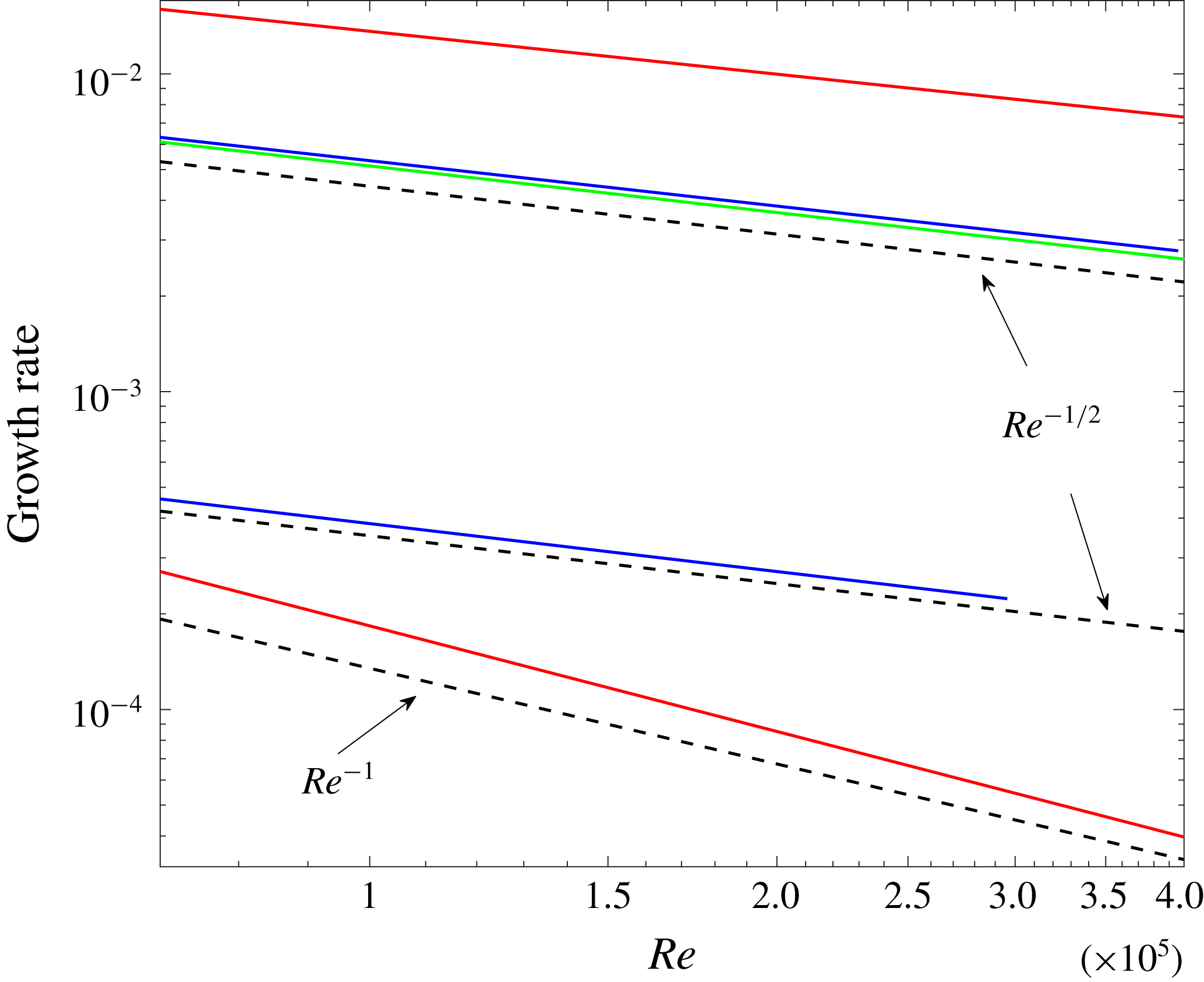
Growth rates from a linear stability analysis of the fully resolved solution are shown in figure 11. The growth rates of the two unstable modes of WK2 decay like
 $Re^{-0.43}$
and
 $Re^{-1.13}$
. This is in good agreement (
 $Re^{-0.42}$
and
 $Re^{-1.12}$
) with the single axial mode approximation of a TW solution (see figure 10), and in rough agreement with the asymptotic
 $Re^{-1/2}$
and
 $Re^{-1}$
scalings of Deguchi & Hall (Reference Deguchi and Hall2016) for the edge and slow instability modes. In spite of the seemingly large values of
 $Re$
used in our numerical calculations, the agreement with the leading-order asymptotic theory is not close. The poor agreement is probably due to higher order corrections associated with small fractional powers of
 $1/Re$
in the asymptotic theory. In this context, it may be noted that even for the TW itself, agreement with the asymptotic theory was only conclusive after calculations in the range
 $1.5\times 10^{4}<Re<1.19\times 10^{6}$
reported in the first part of this paper, whereas previous calculations of WK for the range
 $5\times 10^{3}<Re<1.1\times 10^{4}$
in Ozcakir et al. (Reference Ozcakir, Tanveer, Hall and Overman2016) were rather inconclusive.
A further check on the edge mode is available. A key property of the Deguchi–Hall edge instability mode is that the wave pressure eigenfunction is, to leading order, proportional to the equilibrium wave pressure of the VWI state. Figure 12 shows an excellent agreement between the pressure eigenfunction corresponding to the linearized stability problem and the pressure profile of the equilibrium WK2 state at
 $Re=125\,000$
.
Further, as shown in figure 13(a), the streak component of the eigenfunction associated with the edge states shows that the streak action is concentrated around the critical layer, which is similar to the viscous sublayer structure of the edge states found in Deguchi & Hall (Reference Deguchi and Hall2016).
The growth rates of the unstable modes against
 $Re$
on a log–log scale for WK2 (red), C1 (blue) and C2 (green) at
 $\unicode[STIX]{x1D6FC}=1.55$
. The black dashed lines indicate the asymptotic scalings
 $Re^{-1/2}$
and
 $Re^{-1}$
for comparison. The growth rates for the C1 branch are only shown for
 $Re<3\times 10^{5}$
due to computational storage limitations.
The pressure component of (a) equilibrium solution at
 $\tilde{z}_{0}=2\unicode[STIX]{x03C0}/\unicode[STIX]{x1D6FC}$
at
 $Re=125\,000$
, with corresponding (b) pressure eigenfunction associated with edge mode of WK2.

Roll and streak components of unstable eigenmodes (a)
 $\boldsymbol{\unicode[STIX]{x1D702}}_{1}$
associated with edge and (b)
 $\boldsymbol{\unicode[STIX]{x1D702}}_{2}$
slow modes of WK2 at
 $Re=125\,000$
.

As opposed to the VWI states, all the axial wave harmonics are of the same order in
 $Re$
throughout a shrinking core for the NVC states. Computationally that means more computational space is required for the linear stability analysis at large
 $Re$
values. Using available resources, we limited our attention to the calculation of C2 stability for
 $Re\leqslant 5\times 10^{6}$
to disturbances that have the additional shift-and-rotate symmetry as the base state. The stability calculations for C1 are restricted to
 $Re\leqslant 3\times 10^{5}$
due to computational limitations; these states have no shift-and-rotate symmetry and therefore eigenfunctions of the stability operator do not have this symmetry either. The stability features of C1 are shown in figure 11.
For C1, the stability calculations suggest the existence of two real unstable modes with growth rates scaling like
 $Re^{-0.49}$
and
 $Re^{-0.46}$
. For C2, there is only one real unstable mode with growth rate scaling like
 $Re^{-0.46}$
over the range
 $7\times 10^{4}\leqslant Re\leqslant 5\times 10^{6}$
. The streak components of the eigenfunctions associated with the unstable eigenmodes of C1 and C2 are shown in figure 14. It is clear from figure 14(a,c) that for C2 the most unstable eigenmode is concentrated near the core, while the most unstable eigenmode for C1 is spread throughout the pipe. Also, it is worth noting that the most unstable
 $C$
mode in figure 14(a) has almost a four-fold azimuthally symmetric streak structure quite similar to that of figure 14(c). However the second eigenfunction has an apparent two-fold azimuthal symmetry. Based on these observations, we suspect that at some large
 $Re$
value, the second most unstable C1 eigenvalue which has an eigenfunction spread across the pipe goes through a zero and becomes stable; and that this zero crossing corresponds to an azimuthal-symmetry-breaking bifurcation of C1 from C2 at some large value of
 $Re$
. A confirmation of this scenario requires computations beyond our present resources. If this conjecture holds, only C2 survives as
 $Re\rightarrow \infty$
. Moreover it has only one unstable mode within the class of symmetry-preserving disturbances; this implies that C2 is an edge state in this state space. Furthermore the growth rate for this unstable mode scales like
 $Re^{-1/2}$
which is in surprisingly good agreement with the Deguchi–Hall edge mode predictions since the NVC states have a very different asymptotic structure from the VWI states. However for more general perturbations it is not clear if it would remain an edge state.
The roll and streak components of the unstable eigenmodes (a)
 $\boldsymbol{\unicode[STIX]{x1D702}}_{1}$
associated with the edge and (b)
 $\boldsymbol{\unicode[STIX]{x1D702}}_{2}$
slow modes of C1 at
 $Re=102\,820$
. (c) The roll and streak components of the unstable eigenmode
 $\boldsymbol{\unicode[STIX]{x1D702}}$
of C2 at
 $Re=102\,820$
.

4.3 Linear stability of C2 for constant mean mass flux
All calculations reported thus far correspond to the mean pressure gradient being held fixed. However, through a transformation of the variables and parameters (see (A 8)), a TW solution with the same mean pressure gradient as the base flow
 $\boldsymbol{v}_{\boldsymbol{B}}$
can be mapped onto a TW solution for the same mass flux as
 $\boldsymbol{v}_{\boldsymbol{B}}$
. Details of the mapping are given in appendix A. However, no such transformation exists for the stability modes. Imposition of a constant mean pressure gradient does not preserve mean mass flux and vice versa. Thus, these disturbance modes are fundamentally different. This has been recognized earlier in the literature in a broader context; see for example Soibelman & Meiron (Reference Soibelman and Meiron1991). Our numerical calculations also confirm that constant pressure gradient modes do not satisfy the mass-flux condition (2.8) and vice versa.
We were motivated to conduct a limited linear stability study for constant mass flux in order to compare with the calculations reported in Pringle et al. (Reference Pringle, Duguet and Kerswell2009). As mentioned earlier in § 3, close agreement of the
 $C$
versus
 $Re$
curves shown in figure 2 suggests that the C2 solution curve that we first reported in Ozcakir et al. (Reference Ozcakir, Tanveer, Hall and Overman2016) is a large
 $Re$
continuation of their ‘N2’ solution branch. However, when we attempted to reproduce their constant mass-flux stability results in the vicinity of saddle-node bifurcation point
 $R_{m}\approx 1441$
(
 $Re\approx 2040$
) when
 $\unicode[STIX]{x1D6FC}=1.2$
in the
 $S$
-symmetric space as shown in § 4.3, we noticed some discrepancies. Figure 15 shows stability calculations of N2 performed by Pringle et al. (Reference Pringle, Duguet and Kerswell2009) while figure 16 shows our stability results in the same regime. We find one real and two complex conjugate pairs of unstable eigenvalues on the upper branch that become two real and two complex conjugate pairs of unstable eigenvalues on the lower branch. However Pringle et al. (Reference Pringle, Duguet and Kerswell2009) report three real and a complex conjugate pair of unstable eigenvalues on the upper branch and two real and a complex conjugate pair of unstable eigenvalues on the lower branch. We checked our calculations by significantly increasing the number of modes in each of the radial, azimuthal and axial directions with no change in conclusion. The details of resolution checks can be found in appendix C. At this point, we are unsure about the cause of this discrepancy. One explanation is that, though the
 $C$
versus
 $R_{m}$
curves in figure 2 match closely, N2 is actually different from C2. Another possibility suggested by a referee is potential resolution issues in the Pringle calculations due to computational limitations at the time.
The growth rate calculations for C3 of Pringle et al. (Reference Pringle, Duguet and Kerswell2009) (which is referred to as C2 in this paper) branches at
 $\unicode[STIX]{x1D6FC}=1.2$
under the constant mass-flux constraint. The stability analysis was performed in the
 $R_{2}$
symmetric subspace in the vicinity of the saddle-node bifurcation at
 $R_{m}=1141$
at
 $\unicode[STIX]{x1D6FC}=1.2$
. Each curve indicates either real eigenvalue (solid curves) or a complex conjugate pair (dashed curves) as
 $C$
changes. The black curves correspond to those that are symmetric under
 $S$
, while the grey curves are antisymmetric under
 $S$
. Intersection of the horizontal and vertical dotted lines corresponds to the position of the saddle node, of which the inset is a close-up. Saddle-node bifurcations are observed at
 $C=1.33,1.38,1.385,1.388$
and
 $1.389$
and Hopf bifurcations are observed at
 $1.44,1.47$
and
 $1.50$
.

The growth rates of the constant mass-flux unstable modes of C2 in the vicinity of the saddle-node bifurcation at
 $R_{m}\approx 1141$
at
 $\unicode[STIX]{x1D6FC}=1.2$
. The stability analysis was performed in the two-fold rotational (
 $\mathbb{R}_{2}$
) subspace with
 $\mathbb{S}$
-symmetry. Curves indicate either real eigenvalue (solid curves) or a complex conjugate pair (dashed curves) as
 $C$
changes. Intersection of the horizontal and vertical dotted lines corresponds to the position of the saddle node shown in figure 2. Resolution checks of the unstable growth rates marked by stars at
 $R_{m}=1190$
are given in appendix C.

5 Conclusion
In this paper, we have reported on new numerical computations of TW solutions with shift-and-rotate symmetry. We presented some features of these solutions, including scaling of the lower-branch WK2 with Reynolds number in the range
 $1.5\times 10^{4}<Re<1.19\times 10^{6}$
. Quantitative evidence suggests rather conclusively that the calculated lower-branch WK2 solution is indeed a finite
 $Re$
realization of a VWI state with the expected
 $Re^{-1}$
scale for rolls,
 $O(1)$
scale for streaks and a maximal wave amplitude of
 $O(Re^{-5/6})$
.
From the agreement of
 $c$
versus
 $Re$
relation over a certain range of
 $Re$
for particular axial wavenumber, it appears that the WK2 and C2 solutions are continuations of the so-called ‘N’- and ‘M’-class solutions of Pringle et al. (Reference Pringle, Duguet and Kerswell2009) with two-fold azimuthal symmetry. Their classification is based on fast/slow streak behaviour on a pipe cross-section with the M-class having a double-layer structure of fast and slow streaks across the pipe radius while the N-class have a separation of the fast streaks near the wall and towards the pipe centre. On the other hand, the evidence in this paper and in Ozcakir et al. (Reference Ozcakir, Tanveer, Hall and Overman2016) suggests that the WK2 and C2 solutions are finite
 $Re$
representations of VWI and NVC states respectively. It is very likely that other N- and M-class solutions of Pringle et al. (Reference Pringle, Duguet and Kerswell2009) could also be classified as VWI and NVC states in the asymptotic limit respectively.
Further, we determined computationally the linear stability properties of the TW solutions C1, C2, WK and WK2. We found that at the saddle-node bifurcation points in the
 $c$
–
 $Re$
plane, there is a zero crossing of one real eigenvalue. We confirmed that WK arises as a symmetry-breaking bifurcation from WK2. Our calculations show that C1 continues at least up to
 $Re=2\times 10^{8}$
and gets closer to C2 as
 $Re$
gets larger, and observations on the unstable eigenmodes of C1 and C2 suggest a similar bifurcation scenario. Unfortunately our calculations did not have enough resolution to confirm whether these two branches join at very high values of
 $Re$
.
We also identified Hopf bifurcation points for C1; these will give rise to relative periodic orbits similar to those discussed in Viswanath (Reference Viswanath2007), Duguet et al. (Reference Duguet, Pringle and Kerswell2008a
) and Deguchi & Hall (Reference Deguchi and Hall2016), but we have not pursued them in this paper. Also, it is interesting to note that an initial edge state solution in the form of a WK lower branch has only one real unstable eigenvalue. When it is continued to larger
 $Re>11\,000$
, it gains additional unstable eigenvalues before it joins WK2. We confirmed that these lower-branch TWs have slow and low-dimensional unstable manifolds. Thus, WK2 has two unstable eigenvalues asymptotically scaling as
 $Re^{-0.43}$
and
 $Re^{-1.13}$
, whereas the eigenvalue of C2 scales as
 $Re^{-0.46}$
suggesting their relevance to transition in turbulence. Thus, lower-branch C2 solutions are edge states that form part of the boundary separating laminar and turbulent flows.
Acknowledgements
This work made use of the facilities of NCI under project d77. The authors wish to thank the referees for many constructive comments.
Appendix A. The relation between constant-pressure and mass-flux base flows
Calculations in the literature for the most part use constant flux, i.e. the periodically averaged component of the flux is the same as the Hagen–Poiseuille flow, rather than maintaining the same mean pressure gradient. For TWs, there is a mapping of the Reynolds number and phase speed that maps the constant-pressure TW solution to equivalent constant mass-flux TW. This is well known, and is demonstrated below for completeness. Suppose, for constant flux, the TW solution
 $\bar{\boldsymbol{u}}$
is decomposed as
 $\bar{\boldsymbol{u}}=\tilde{\boldsymbol{v}}(r,\unicode[STIX]{x1D703},z-c_{m}t)+w_{0}(r)\hat{\boldsymbol{z}}$
, where
 $$\begin{eqnarray}w_{0}(r)=-\frac{Q_{0}R_{m}}{4}(1-r^{2})\end{eqnarray}$$
is a pressure eigenfunction Poisseuille correction, and therefore there is no averaged flux contribution from
 $\tilde{\boldsymbol{v}}$
. The constancy of the mass flux determines
 $Q_{0}$
in terms of
 $\tilde{\boldsymbol{v}}$
. Substituting the expression for
 $\bar{\boldsymbol{u}}$
into the Navier–Stokes equations gives
 $$\begin{eqnarray}-c_{m}\tilde{\boldsymbol{v}}_{z}+\tilde{\boldsymbol{v}}\boldsymbol{\cdot }\unicode[STIX]{x1D735}\tilde{\boldsymbol{v}}+(w_{0}\hat{\boldsymbol{z}}+\boldsymbol{v}_{\boldsymbol{B}})\boldsymbol{\cdot }\unicode[STIX]{x1D735}\tilde{\boldsymbol{v}}+\tilde{\boldsymbol{v}}\boldsymbol{\cdot }\unicode[STIX]{x1D735}(w_{0}\hat{\boldsymbol{z}}+\boldsymbol{v}_{\boldsymbol{B}})=-\unicode[STIX]{x1D735}\bar{p}+\frac{1}{R_{m}}\unicode[STIX]{x0394}\tilde{\boldsymbol{v}},\end{eqnarray}$$
where
 $c_{m}$
and
 $R_{m}$
denote the phase speed and the mean Reynolds number, respectively, for the constant mean mass-flux calculations. We find
 $$\begin{eqnarray}w_{0}\hat{\boldsymbol{z}}+\boldsymbol{v}_{\boldsymbol{B}}=\left(1-\frac{Q_{0}R_{m}}{4}\right)(1-r^{2})\hat{\boldsymbol{z}}=\unicode[STIX]{x1D707}\boldsymbol{v}_{\boldsymbol{ B}},\quad \text{where }\unicode[STIX]{x1D707}=\left(1-\frac{Q_{0}R_{m}}{4}\right).\end{eqnarray}$$
This implies that
 $$\begin{eqnarray}-c_{m}\tilde{\boldsymbol{v}}_{z}+\tilde{\boldsymbol{v}}\boldsymbol{\cdot }\unicode[STIX]{x1D735}\tilde{\boldsymbol{v}}+\unicode[STIX]{x1D707}\boldsymbol{v}_{\boldsymbol{B}}\boldsymbol{\cdot }\unicode[STIX]{x1D735}\tilde{\boldsymbol{v}}+\tilde{\boldsymbol{v}}\boldsymbol{\cdot }\unicode[STIX]{x1D735}\unicode[STIX]{x1D707}\boldsymbol{v}_{\boldsymbol{B}}=-\unicode[STIX]{x1D735}\bar{p}+\frac{1}{R_{m}}\unicode[STIX]{x0394}\tilde{\boldsymbol{v}}.\end{eqnarray}$$
Next we define new variables
 $\tilde{\boldsymbol{v}}=\unicode[STIX]{x1D707}\boldsymbol{v}$
,
 $\bar{p}=\unicode[STIX]{x1D707}^{2}q$
and divide (A 4) by
 $\unicode[STIX]{x1D707}^{2}$
, so that
 $$\begin{eqnarray}-\frac{c_{m}}{\unicode[STIX]{x1D707}}\boldsymbol{v}_{z}+\boldsymbol{v}\boldsymbol{\cdot }\unicode[STIX]{x1D735}\boldsymbol{v}+\boldsymbol{v}_{\boldsymbol{B}}\boldsymbol{\cdot }\unicode[STIX]{x1D735}\boldsymbol{v}+\boldsymbol{v}\boldsymbol{\cdot }\unicode[STIX]{x1D735}\boldsymbol{v}_{\boldsymbol{B}}=-\unicode[STIX]{x1D735}q+\frac{1}{R_{m}\unicode[STIX]{x1D707}}\unicode[STIX]{x0394}\boldsymbol{v};\quad \unicode[STIX]{x1D735}\boldsymbol{\cdot }\boldsymbol{v}=0,\end{eqnarray}$$
which is the same as equation (2.6) for TWs with constant mean pressure gradient provided we identify
 $$\begin{eqnarray}\frac{c_{m}}{\unicode[STIX]{x1D707}}=c,\quad \unicode[STIX]{x1D707}R_{m}=Re.\end{eqnarray}$$
In order to determine
 $Q_{0}$
and hence
 $\unicode[STIX]{x1D707}$
(noting the relation (A 3)), we invoke the mass-flux constraint
 $$\begin{eqnarray}\unicode[STIX]{x1D707}\int _{0}^{1}(\boldsymbol{v}\boldsymbol{\cdot }\hat{\boldsymbol{z}})_{00}r\,\text{d}r=-\int _{0}^{1}w_{0}(r)r\,\text{d}r=\frac{Q_{0}R_{m}}{4}\int _{0}^{1}(1-r^{2})r\,\text{d}r=\frac{Q_{0}R_{m}}{16},\end{eqnarray}$$
which together with (A 3) implies that
 $$\begin{eqnarray}Q_{0}=\frac{16}{R_{m}}\frac{{\mathcal{I}}}{1+4{\mathcal{I}}}\quad \text{and}\quad \unicode[STIX]{x1D707}=\frac{1}{1+4{\mathcal{I}}},\quad \text{where }{\mathcal{I}}=\int _{0}^{1}\overline{(\boldsymbol{v}\boldsymbol{\cdot }\hat{\boldsymbol{z}})}r\,\text{d}r,\end{eqnarray}$$
where
 $\overline{(~~~~)}$
refers to azimuthal and axial period averaging.
Since the numerical evidence suggests that the Jacobian associated with (2.6) is non-singular except at bifurcation points, we therefore have a locally unique solution ensuring that the solution
 $\boldsymbol{v}$
of (A 5) is the same constant-pressure solution of (2.6), provided we relate
 $(c_{m},R_{m})$
to
 $(c,Re)$
through (A 5) and (A 7). Thus the numerical calculation reported here for constant mean pressure gradient can be related to constant mass-flux calculations that appear elsewhere in the literature, see for example Pringle et al. (Reference Pringle, Duguet and Kerswell2009), and the full transformation corresponds to
 $$\begin{eqnarray}(\bar{\boldsymbol{u}},\bar{p},c_{m};R_{m})=\left(\unicode[STIX]{x1D707}\boldsymbol{u}-4\unicode[STIX]{x1D707}{\mathcal{I}}(1-r^{2})\hat{\boldsymbol{z}},\unicode[STIX]{x1D707}^{2}p,\unicode[STIX]{x1D707}c,\frac{Re}{\unicode[STIX]{x1D707}}\right)\quad \text{with }\unicode[STIX]{x1D707},{\mathcal{I}}\text{ in }(\text{A}\,7).\end{eqnarray}$$
It is to be noted that
 $\unicode[STIX]{x1D707}$
in (A 7) is related to the mean flow velocity
 $W_{m}$
appearing through the relation
 $\unicode[STIX]{x1D707}=1/2W_{m}$
. Therefore (A 8) is equivalent to
 $R_{m}=2W_{m}Re$
and
 $c_{m}=c/2W_{m}$
.
The relative errors found by comparing the numerical solutions at various levels of truncation
 $(N_{2},M_{2},P_{2})$
with the baseline calculations with
 $(N_{1},M_{1},P_{1})=(220,20,5)$
for the WK2 curve for
 $(Re,\unicode[STIX]{x1D6FC})=(710\,000,1.55)$
.

The relative errors found by comparing the numerical solutions at various levels of truncation
 $(N_{2},M_{2},P_{2})$
with the baseline calculations with
 $(N_{1},M_{1},P_{1})=(165,18,5)$
for the C2 curve for
 $(Re,\unicode[STIX]{x1D6FC})=(191\,020,1.55)$
.

Appendix B. Resolution checks for TWs
In this appendix, we confirm the accuracy of the WK2, C1 and C2 TW calculations by comparing solutions at different truncations
 $(N,M,P)$
. We performed detailed resolution checks at a few
 $Re$
values when
 $k_{0}=2,\unicode[STIX]{x1D6FC}=1.55$
. Results shown in the tables 2–7 display relative errors between the two compared solutions for phase speed, velocity components and pressure. In each table, we compare a TW solution calculated at truncation levels
 $(N_{1},M_{1},P_{1})$
and
 $(N_{2},M_{2},P_{2})$
.
Let
 $\boldsymbol{X}_{1}$
be the solution at truncation level
 $(N_{1},M_{1},P_{1})$
and
 $\boldsymbol{X}_{2}$
the solution at truncation level
 $(N_{2},M_{2},P_{2})$
, where
 $N_{1}\leqslant N_{2}$
,
 $M_{1}\leqslant M_{2}$
and
 $P_{1}\leqslant P_{2}$
. The comparison is made by taking the difference between these two solutions by injecting the lower resolution solution
 $\boldsymbol{X}_{1}$
into the higher dimension by adding zeros in the Fourier
 $\unicode[STIX]{x1D703}$
and
 $z$
domain. Then each velocity component and pressure are computed in the real radial domain at the same radial collocation points using interpolation in the radial domain while keeping the solution in the Fourier
 $\unicode[STIX]{x1D703}$
and
 $z$
space. The error comparison is done by computing relative errors using the infinity norm for each component in Fourier space separately. We denote
 $\boldsymbol{u}=\{u_{jkl}|0\leqslant j\leqslant N,0\leqslant k\leqslant M,0\leqslant l\leqslant P\}$
and define
 $\boldsymbol{v}$
and
 $\boldsymbol{w}$
in the same manner.
It is clear from the findings that when
 $Re$
gets larger, more radial N and azimuthal M modes are required to get good accuracy for WK2, C1 and C2, while a low value of
 $P=5$
is enough to achieve remarkable accuracy due to the single dominating axial mode property of VWI states.
The relative errors found by comparing the numerical solutions at various levels of truncation
 $(N_{2},M_{2},P_{2})$
with the baseline calculations with
 $(N_{1},M_{1},P_{1})=(220,20,8)$
for the C2 curve for
 $(Re,\unicode[STIX]{x1D6FC})=(1\,026\,020,1.55)$
.

The relative errors found by comparing the numerical solutions at various levels of truncation
 $(N_{2},M_{2},P_{2})$
with the baseline calculations with
 $(N_{1},M_{1},P_{1})=(220,20,12)$
for the C2 curve for
 $(Re,\unicode[STIX]{x1D6FC})=(8\,241\,020,1.55)$
.

The relative errors found by comparing the numerical solutions at various levels of truncation
 $(N_{2},M_{2},P_{2})$
with the baseline calculations with
 $(N_{1},M_{1},P_{1})=(220,20,12)$
for the C1 curve for
 $(Re,\unicode[STIX]{x1D6FC})=(1\,261\,020,1.55)$
.

The relative errors found by comparing the numerical solutions at various levels of truncation
 $(N_{2},M_{2},P_{2})$
with the baseline calculations with
 $(N_{1},M_{1},P_{1})=(220,20,12)$
for the C1 curve for
 $(Re,\unicode[STIX]{x1D6FC})=(3\,263\,020,1.55)$
.

The relative errors found by comparing the numerical solutions at various levels of truncation
 $(N_{2},M_{2},P_{2})$
with the baseline calculations with
 $(N_{1},M_{1},P_{1})=(125,16,5)$
for the unstable eigenvalues
 $\unicode[STIX]{x1D706}_{1}=0.01227,\unicode[STIX]{x1D706}_{2}=0.00014474$
for the WK2 curve for
 $(Re,\unicode[STIX]{x1D6FC})=(125\,000,1.55)$
. Note that
 $\unicode[STIX]{x1D706}_{1}$
corresponds to WK2 edge modes; the cross-sectional velocity and pressure profiles of the corresponding eigenfunction are given in figures 12 and 13.

The relative errors found by comparing the numerical solutions at various levels of truncation
 $(N_{2},M_{2},P_{2})$
with the baseline calculations with
 $(N_{1},M_{1},P_{1})=(165,16,8)$
for the unstable eigenvalues
 $\unicode[STIX]{x1D706}_{1}=0.0039247,\unicode[STIX]{x1D706}_{2}=0.00027827$
for the C1 curve for
 $(Re,\unicode[STIX]{x1D6FC})=(191\,020,1.55)$
.

The relative errors found by comparing the numerical solutions at various levels of truncation
 $(N_{2},M_{2},P_{2})$
with the baseline calculations with
 $(N_{1},M_{1},P_{1})=(145,16,8)$
for the only unstable eigenvalue (
 $\unicode[STIX]{x1D706}_{1}=0.0037345$
) for the C2 curve for
 $(Re,\unicode[STIX]{x1D6FC})=(191\,020,1.55)$
.

The relative errors found by comparing the numerical solutions at various levels of truncation
 $(N_{2},M_{2},P_{2})$
with the baseline calculations with
 $(N_{1},M_{1},P_{1})=(65,16,12)$
for the unstable eigenvalues
 $\unicode[STIX]{x1D706}_{1}=0.045528+0.15917i$
,
 $\unicode[STIX]{x1D706}_{2}=0.043037+0.42324i$
,
 $\unicode[STIX]{x1D706}_{3}=0.015814$
,
 $\unicode[STIX]{x1D706}_{4}=0.014294$
, for the mass-flux-preserving lower C2 branch for
 $\unicode[STIX]{x1D6FC}=1.2$
given in figure 2 for
 $(R_{m},C)=(1190,1.4218)$
. These unstable eigenvalues are marked with stars in figure 16.

The relative errors found by comparing the numerical solutions at various levels of truncation
 $(N_{2},M_{2},P_{2})$
with the baseline calculations with
 $(N_{1},M_{1},P_{1})=(65,16,12)$
for the unstable eigenvalues
 $\unicode[STIX]{x1D706}_{1}=0.060732+0.15325i$
,
 $\unicode[STIX]{x1D706}_{2}=0.055847+0.42618i$
for the mass-flux-preserving upper C2 branch for
 $\unicode[STIX]{x1D6FC}=1.2$
given in figure 2 for
 $(R_{m},C)=(1190,1.3568)$
. These unstable eigenvalues are marked with stars in figure 16.

Appendix C. Details of the stability problem and resolution checks for the growth rates
For small
 $Re$
values a standard eigenvalue solver is used to compute eigenvalues with good numerical accuracy. However, when
 $Re$
is large, this becomes a numerical challenge since a calculation of the TWs for high values of
 $Re$
is computationally expensive due to the size of the Jacobian needed to resolve the solution. For the linear stability of these converged TW solutions at high
 $Re$
, a higher resolution has to be chosen; therefore the matrix created from the linearized equation (2.6) will have to be at least as big as the Jacobian for the converged TW. For example, when
 $Re=125\,000$
, TWs are calculated with
 $(N,M,P)=(125,16,5)$
. Using the linearized equation (2.6) for the stability analysis about these TWs at the same truncation level will create a matrix of size
 $68\,419\times 68\,419$
for shift-and-reflect symmetric states WK, C1 and
 $34\,399\times 34399$
for WK2 and C2 which have additional shift-and-rotate symmetry. For this reason, we solve the eigenvalue problem on a coarse grid only at a few small
 $Re$
values around the bifurcation points in figure 1. The resulting eigenvalues are useful in determining the generic features of the system, i.e. number of unstable real and complex eigenvalues. Then, the first few most unstable eigenvalues and the corresponding eigenfunctions are used as rough initial guesses
 $(\unicode[STIX]{x1D706}_{0},\boldsymbol{y}_{0})$
for the stability problem at larger
 $Re$
in a Newton iteration scheme to solve for a specific eigenvalue–eigenvector pair
 $(\unicode[STIX]{x1D706},\boldsymbol{y})$
satisfying
 $A\boldsymbol{y}-\unicode[STIX]{x1D706}\boldsymbol{y}=0$
. Through a continuation procedure in
 $Re$
, this method allows us to compute eigenvalues and eigenfunctions very accurately using GMRES at each Newton iteration without constructing a huge matrix
 $\unicode[STIX]{x1D63C}$
. It should be noted that in the parameter space (
 $Re$
or
 $c$
) when a complex conjugate pair of eigenvalues in the form
 $\unicode[STIX]{x1D706}=\text{Re}\unicode[STIX]{x1D706}\pm \text{i}\text{Im}\unicode[STIX]{x1D706}$
, with corresponding eigenvectors
 $\boldsymbol{y}=\text{Re}\boldsymbol{y}\pm \text{i}\text{Im}\boldsymbol{y}$
, coalesce and become real, the nonlinear Newton solver was modified by treating
 $\text{Re}\unicode[STIX]{x1D706},\text{Im}\unicode[STIX]{x1D706},\text{Re}\boldsymbol{y}$
and
 $\text{Im}\boldsymbol{y}$
as distinct real unknowns. This resulted in a Jacobian matrix
 $\hat{\unicode[STIX]{x1D63C}}$
that is twice the size of matrix
 $\unicode[STIX]{x1D63C}$
, but allows for the continuation of an eigenvalue–eigenvector pair past the transition point from real to complex, or vice versa.
Results shown in the tables display the relative errors at a few
 $Re$
values between the two compared solutions for the
 $i$
th most unstable eigenvalue (growth rate)
 $\unicode[STIX]{x1D706}_{i}$
, velocity components
 $(\tilde{u_{i}},\tilde{v_{i}},\tilde{w_{i}})$
of the corresponding eigenfunction
 $y_{i}$
. In each table, we compare linear stability calculations of a given TW solution calculated at truncation levels
 $(N_{1},M_{1},P_{1})$
and
 $(N_{2},M_{2},P_{2})$
using the same approach used in appendix B.
In tables 8–10 we confirm the accuracy of the growth rate calculations for WK2, C1 and C2 TWs shown in figure 11 by comparing solutions at different truncations
 $(N,M,P)$
, where we imposed constant pressure gradient condition. The growth rate results presented are accurate to at least seven significant digits based on these computational verifications, while the corresponding eigenfunctions are only accurate to at least two digits.
Furthermore, in tables 11 and 12, we present numerical resolution checks for linear stability results under constant mass-flux condition for the unstable growth rates marked with stars in figure 16 at
 $Re=1190$
. The results provide numerical evidence for the accuracy of calculations presented in this paper.



